Control and EMS of a Grid-Connected Microgrid with Economical Analysis

1
Faculty of Engineering and Applied Science, University of Ontario Institute of Technology, 2000 Simcoe Street North, Oshawa, ON L1H7K4, Canada
2
Electrical Engineering Department, Faculty of Engineering, Assiut University, Assiut 71515, Egypt
3
Faculty of Energy Systems and Nuclear Science, University of Ontario Institute of Technology, 2000 Simcoe Street North, Oshawa, ON L1H7K4, Canada
*
Author to whom correspondence should be addressed.
Energies 2018, 11(1), 129; https://doi.org/10.3390/en11010129
Submission received: 24 November 2017
/
Revised: 29 December 2017
/
Accepted: 3 January 2018
/
Published: 5 January 2018
Abstract
:Recently, significant development has occurred in the field of microgrid and renewable energy systems (RESs). Integrating microgrids and renewable energy sources facilitates a sustainable energy future. This paper proposes a control algorithm and an optimal energy management system (EMS) for a grid-connected microgrid to minimize its operating cost. The microgrid includes photovoltaic (PV), wind turbine (WT), and energy storage systems (ESS). The interior search algorithm (ISA) optimization technique determines the optimal hour-by-hour scheduling for the microgrid system, while it meets the required load demand based on 24-h ahead forecast data. The control system consists of three stages: EMS, supervisory control and local control. EMS is responsible for providing the control system with the optimum day-ahead scheduling power flow between the microgrid (MG) sources, batteries, loads and the main grid based on an economic analysis. The supervisory control stage is responsible for compensating the mismatch between the scheduled power and the real microgrid power. In addition, this paper presents the local control design to regulate the local power, current and DC voltage of the microgrid. For verification, the proposed model was applied on a real case study in Oshawa (Ontario, Canada) with various load conditions.
1. Introduction
The main goals of sustainability in the energy system are economic operation, reliability, and environmental impact. Recently, the concept of microgrid (MG) and its applications have become important topics. MG is a small grid that can aggregate conventional generators, renewable energy systems (RESs), and energy storage systems (ESS) along with different loads, to form a self-sufficient and flexible system [1,2,3]. MG can operate in grid-connected mode or in islanded mode (i.e., for remote areas and in case of grid failure) [4]. One of the main advantages of the MG technology is that it can supply the customers with the electricity demand and guarantee the reliability and intelligence of the power system.
There are various topologies and designs for MGs in the literature. An AC MG is the standard choice for MG designers [5,6,7] due to the flexibility to transform AC voltage level into other levels, in addition to the majority of the loads being AC type. Nowadays, due to the increase of using DC loads, DC MGs have been created due to their advantages in terms of efficiency and cost reduction [8,9,10]. However, to reduce the amount of multiple conversion stages and to connect the AC and DC sources and loads in a efficient/economic way, AC/DC MGs have become an ideal choice to connect the MGs [11].
There are many challenges that face microgrids operation. The first challenge is to minimize the operational cost of the MG. Secondly, the intermittency of RESs such as photovoltaic (PV) and wind turbine (WT) because of the weather variation which may cause power imbalance and power-quality problems. Therefore, the decision makers are focusing on finding a solution to make the MG operate in a stable and economic way.
To operate the MG in an economic and reliable manner there are two steps to be considered. The first is to select the best connection to the physical model components, which include RES, ESS, loads, grid components (i.e., transformers, transmission lines and circuit breakers) and power converters which connect all the system components together [12]. The second step is to design the suitable control system to ensure the stability, reliability, and economic operation of the MG. The proposed control system consists of two parts: scheduling and control.
The energy management system (EMS) plays a key role in controlling the generation and/or flow of power in microgrids and thus minimizes the operating cost. EMS controls the power flow in the MG based on optimal cost and provides the scheduled, reference values to the local controller of the MG. The power scheduling problem to provide reference values to the local controllers has been studied before [12,13,14]. However, they focused only on the action of the current values, and also did not take into consideration the cost minimization [15]. Reference [16] suggests that the first priority for load demand is to be supplied from the MG sources as the utility grid will be the final choice. They did not consider market electricity prices. Other papers have focused on the off-line scheduling of the power flow of MG. But they do not consider the mismatch between the scheduled power based on the forecasted data profile and the dynamic operation of the control devices and the generated power profiles [17,18,19].
Many optimization algorithms have been proposed to solve the cost minimization problem. These methods include game theory [20], mixed integer linear programming (MILP) [21], and heuristic optimization methods [22]. Heuristic optimization algorithms are among the most common techniques used by researchers due to: simplicity, flexibility, not relying on derivativeness, and the ability of achieving the near-optimal value for the fitness function. There are several types of heuristic algorithms that are used in EMS such as genetic algorithm (GA), simulated annealing algorithm (SA), cuckoo search algorithm (CSA), particle swarm optimization (PSO) and interior search algorithm (ISA). Ref. [23] offers a comparison among these methods and concludes that ISA is the best heuristic optimization technique to solve the cost minimization problem.
Several control models consider RES as non-dispatchable resources, and therefore, the ESS is used to balance the shortage between the generation and the demand [24,25]. They neglect the feed-in-tariff (FIT) constraint of the main grid which imposes a limit for purchasing power from any MG. Therefore, if the generated power from the MG is higher than these limits, the RES should reduce the generated power to keep the system balanced. The proposed control method can work in two operating strategies: grid interactive mode and grid non-interactive mode to maintain system stability. The grid non-interactive mode requires that each RES works as a non-dispatchable supply which is useful if the MG’s generated power is within the main grid constraints. The other mode, grid interactive is used in large MGs. It considers each RES as a dispatchable supply, which means that the RES can be controlled depending on the system objectives and constraints. In this paper, a small MG is proposed, therefore the MG operates in non-interactive mode, although the control system is designed to work for both operating strategies.
This paper proposes an economic operating strategy of MGs to minimize the operating cost based on 24-h ahead forecast data. The EMS is responsible for predicting the day ahead generated power and load demand based on wavelet neural network (WNN) method. In addition, the optimal power flow is calculated based on economic analysis using heuristic optimization method. It presents a local control strategy to control the voltage and power of the MG and to enhance the stability of the system in the dynamic mode. Supervisory control is integrated to the proposed control model to compensate the mismatch between the scheduled power flow and the real power flow by adjusting the reference power of the ESS.
2. Microgrid Structure and Operation
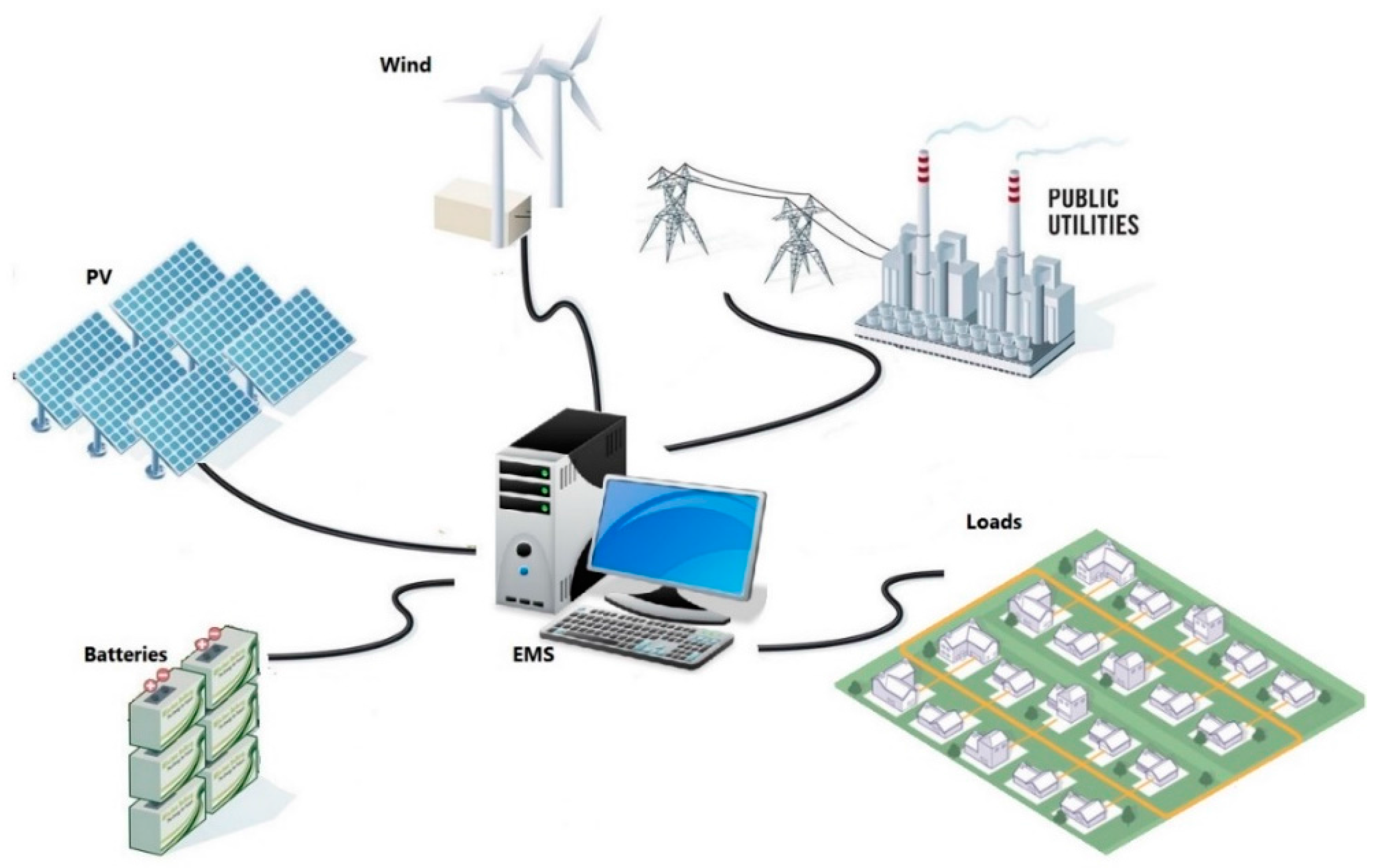
The proposed MG is shown in Figure 1, which consists of a WT, PV generator, battery-based ESS and the load demand. The MG works in grid-connected mode.
As mentioned before, this research proposes an AC/DC MG to reduce the number of conversion stages. The main grid is connected to the AC bus, so it controls the voltage and frequency in the AC bus, and manages any unbalance between the generated and consumed power. On the other hand, the distributed energy resources (DERs) are connected to the DC bus, and because of the variation of the generated power the DC bus must be regulated by the local controller. In this case, DC loads can be connected to the DC bus and AC loads can be connected to the AC bus. The power can be transferred between AC and DC buses by a bidirectional converter.
The EMS sends the scheduled reference power to the controllers to control the power flow in the MG based on the optimization algorithm. These reference values could be defined by two types of operation (grid-interactive or grid non-interactive strategy) [26]. In grid non-interactive mode, the RESs follow the maximum power point tracking (MPPT) algorithm set point and do not take into consideration the scheduled reference power from the EMS. Otherwise, when in grid-interactive mode the RES will follow the EMS’s reference power after being adjusted by the supervisory control.
With respect to Ontario’s FIT program, the utility grid has a power limit to accept power from an external MGs. If there is any surplus power from a MG and its transferred power to the main utility grid has reached its maximum limit, the MG will work in the grid-interactive strategy to balance the power in the power system.
The MG configuration as shown in Figure 2 consists of three parts:
- (1)
- EMS which gives the day-ahead scheduled power;
- (2)
- Design of the local control model to control the power and voltage of the entire system to satisfy the system stability; and
- (3)
- Adjusting the reference power using the supervisory control.
2.1. EMS (Day-Ahead Scheduling)
This part discusses the EMS strategy that used in the proposed MG. EMS is responsible for providing the control system with the optimum day-ahead scheduling power flow between the MG sources, batteries, loads and the main grid based on an economic analysis. The EMS consisted of two parts: the hourly load and weather forecasting for the day-ahead and the optimal power flow in the MG based on heuristic optimization technique.
2.1.1. Weather and Load Forecasting
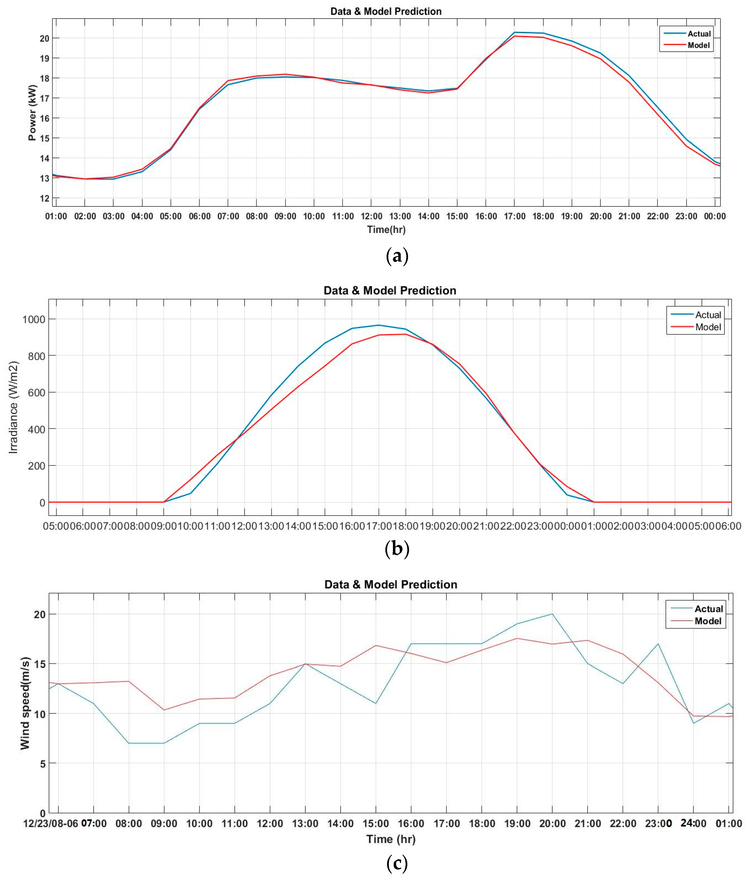
The day-ahead forecasting stage provides the optimization stage with the necessary input data. The forecasting tool predicts the load demand and the weather conditions (irradiance and wind speed which are the input parameters to the PV and WT models respectively). The more accurate the forecasting system the more efficient the EMS. There are many techniques have been used in the forecasting stage to minimize the forecasting error [27,28,29].One of the most accurate techniques is WNN which has been used to predict the day-ahead load demand and weather conditions [30]. Figure 3 illustrates the results from the forecasting model.
2.1.2. Economic Power Flow Optimization
To determine the optimal output power set points for DERs, an efficient optimization method has been proposed. The purpose of the EMS is to minimize the operating cost. Thus, it aims to purchase the power from the grid during the off-peak time, when electricity prices are at their lowest, to store the surplus power in the ESS. This power can be used again to cover the shortage from the MG during the high peak period. On the other hand, if the load demand is smaller than the MG generated power, the surplus power from the RES and ESS will be sold to the grid during high peak periods. The ISA has been used to minimize the operating cost. It chooses the best period to sell/purchase the power to/from the grid and to charge/discharge the ESS to minimize the total operating cost during the day.
As shown in Figure 2, the input parameters to the optimization method are generated power of the PV and WT, load demand, state of charge (SOC) of the battery, the grid tariff and system constraints. The output variables of the ISA are the scheduled power for the next day based on the minimum operating cost. The system constraints and the objectives are as follows:
Objective Function
The objective function of the EMS is used to determine the total operating cost of the proposed MG. ISA has been presented to minimize this cost based on optimal economic power flow. The cost function can be determined as follows:
The time of the optimization method is T (24-h) with time interval t (i.e., 1 h). The input variables and parameters of the optimization model is presented in Table 1. In order to minimize the objective function, ISA optimization choose the optimum set point for the PV, WT and ESS. Also, it decides when exactly the power will be purchased/sold from/to the grid.
System Constraints
To solve the optimization problem, the following constraints and limits should be considered in the optimization process. These technical power limits control the state variables of the optimization method.
(a) System Power Balance
Power balance equation identify the relationship between the generated power and load power in the MG at each time interval:
There are losses on the MG due to converter and transmission lines etc. But these losses are not considered as the supervisor controller adjusts any mismatch between the output power of the EMS and the dynamic model.
(b) DER Constraints
To maintain the stability of system, the output power of the DER must be within the convenient limits. Also, the charging or discharging power of the battery and the amount of stored energy must be limited to prevent any damage and to maximize the lifetime of the battery:
(c) Heuristic Optimization Technique
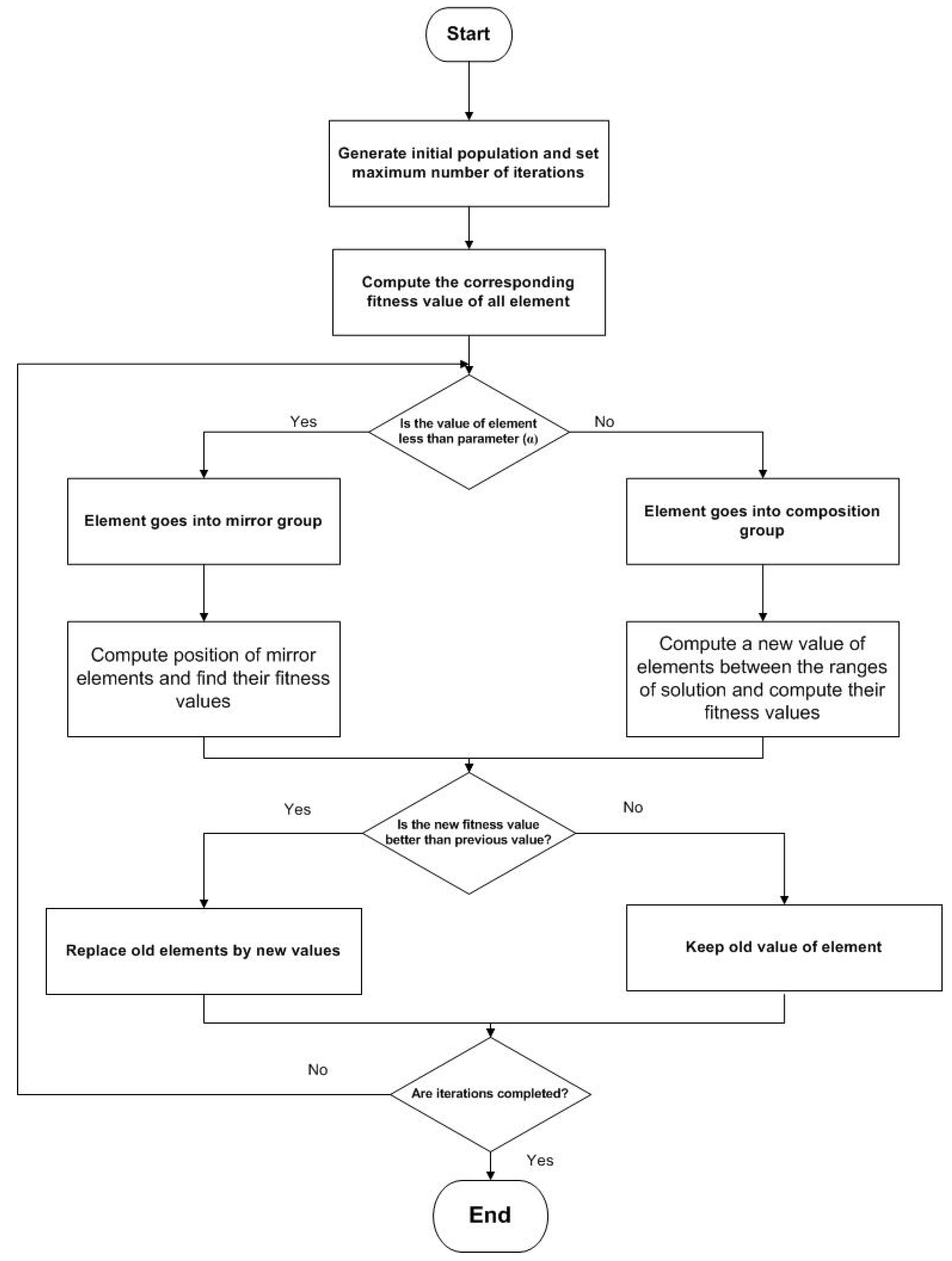
Heuristic optimization technique is one of the powerful optimization methods to determine the optimal power flow. ISA is one of the heuristic optimization techniques which carry out a trade off between accuracy and optimization time range. ISA is a new, fast, reliable, and flexible method given in Ref. [31]. The state variables of ISA are the output power of each DER of the MG at each time interval for one day. The flowchart of ISA optimization is illustrated in Figure 4.
ISA is described in the following steps [32]:
Step 1: generate the initial population of the input variables randomly within the given limits. Then calculate the fitness value for these chosen variables, where is the iteration number and is the population number.
Step 2: find the minimum fitness value at each iteration and the element which has the minimum fitness value is called the current best ().
Step 3: The other elements are divided randomly into two groups, composition and mirror group. The elements go to the composition group when , else they go to the mirror group.
Where between (0,1) and they are a random number, is a parameter which is tuned with respect to ref. [30].
Step 4: For the elements in composition group, change the elements randomly within the range of limited constraint (lower bounds (LB) and upper bounds (UB)):
Step 5: In the mirror group, put a mirror between each element and the current best element randomly. Use Equation (8) to evaluate the position of the mirror:
The new element location depends on the location of the mirror. Use Equation (9) to calculate it:
Step 6: Search around the current best location using Equation (10) to get a new current best location:
where λ is a scale factor and it is equal 0.01 × (UB − LB).
Step 7: Calculate the fitness function of the new and old element. If the fitness value of the new element is less than the old one, replace it, else keep the old element.
Step 8: Repeat these steps from 2 to 7 until reach to the maximum number of iterations.
2.2. Local Controllers
The proposed MG is AC/DC hybrid system which works in grid-connected mode as shown in Figure 2. Therefore, the DC and AC bus voltages must be controlled to protect the loads from voltage variations. In grid-connected mode, the AC bus voltage and frequency are fixed by the grid as mentioned earlier. The local controller controls the local power, current and DC voltage of the MG where the purpose of the local controller is to follow the set point of the supervisory controller.
There are two types of operation for DERs, grid-interactive and non-interactive. The operating mode depends on the case study and the operating conditions. If the surplus power generated from the MG is more than the FIT program power limits, the sold power must not exceed the grid active power constraints. In this case, the MG will operate in the grid-interactive mode. The generated power from RES does not follow the MPPT algorithms and follows the scheduled power reference by EMS, to insure the system stability. In the non-interactive operating mode, the generated power from the RESs follows the MPPT algorithm to ensure extracting the maximum generated power from each RES. In this paper, the proposed model of RESs is smaller than the active power limits of the grid, therefore, the RESs operate in non-interactive mode.
There are four converters in the proposed model. Three converters connect the RES and ESS with the DC bus and a DC/AC bidirectional converter (grid side converter) connects the DC bus to the AC bus.
The grid side converter is responsible for two tasks: (1) to regulate the DC bus voltage to 500 V and (2) to synchronize the MG components with the main grid at the point of common coupling using phase locked loop (PPL) as shown in Figure 5. The other three converters are responsible for: (1) controlling the power generated from each DER; and (2) connecting the DERs to the DC bus by boosting the DC voltage or converting the AC voltage to DC voltage. Also, the ESS converter is a bidirectional converter which controls the charging and discharging power of the battery according to the predefined reference set point.
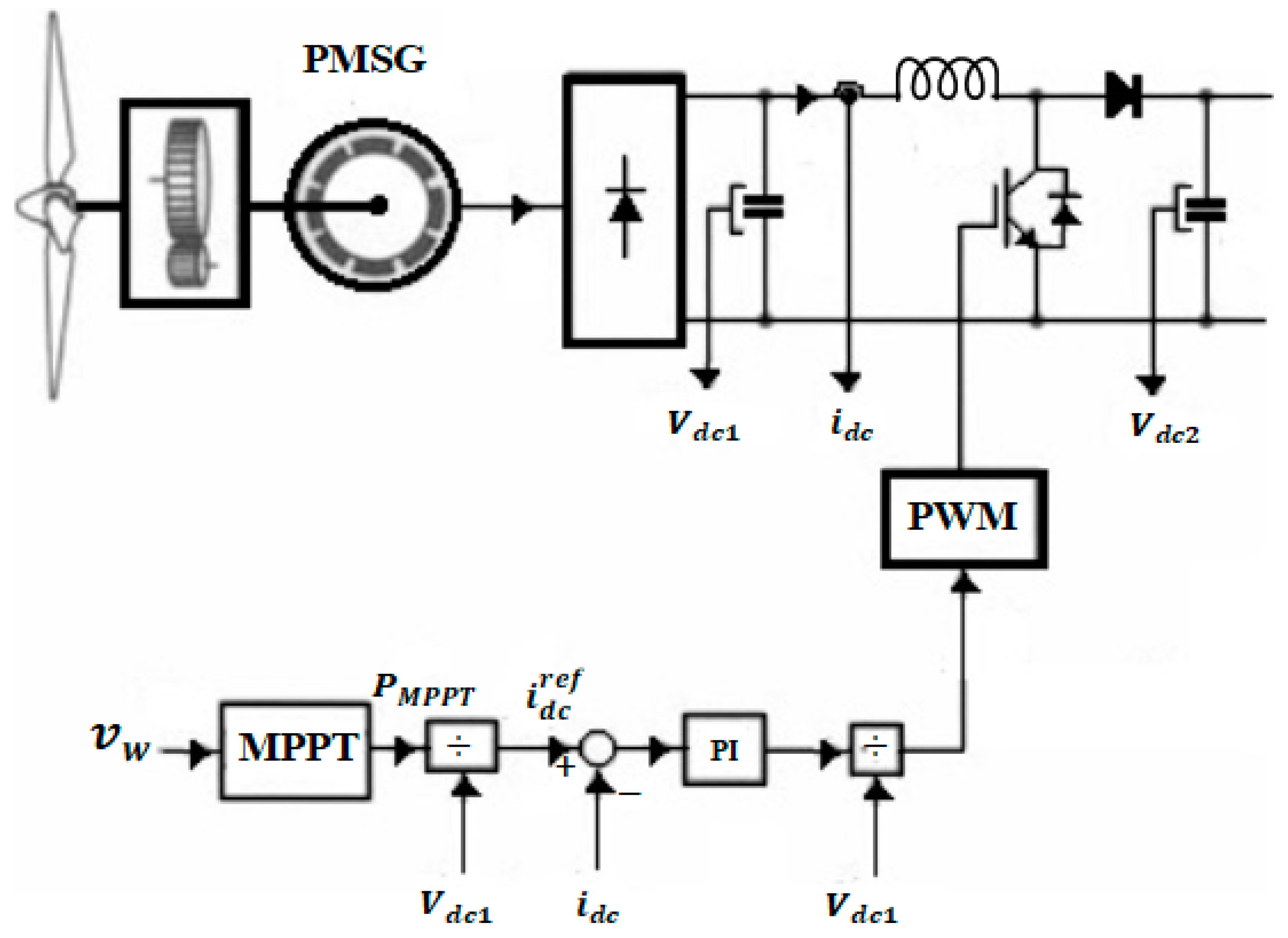
Figure 6 shows the block diagram of the WT generation system using a DC/DC boost converter with a three-phase diode rectifier [33], which is used to connect the WT generator with the DC bus and to control the power output from the permanent magnet synchronous generator (PMSG). Using this converter reduces the cost of the system by reducing the number of conversion stages in addition to the simplicity of its control. Three variables should be controlled: the DC bus voltage, the generator active power, and the grid reactive power. The DC bus voltage and the grid reactive power are controlled by the inverter as shown in Figure 5. The generated power of the PMSG is controlled by regulating the duty cycle (D) of the boost converter via a proportional integrator (PI) controller. Ref. [34] presents the MPPT algorithm for the WT generator.
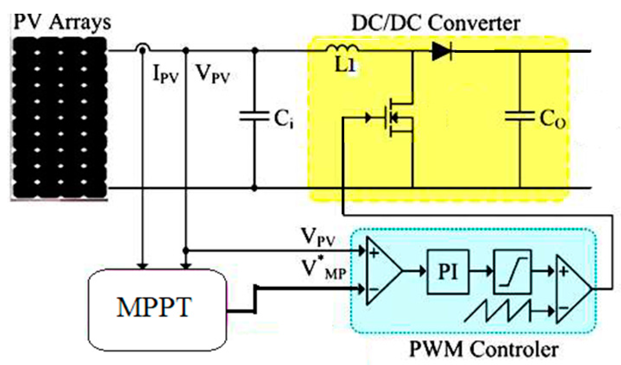
Figure 7 illustrates the PV connection to the MG. A DC/DC boost converter of PV system has two tasks [35]: (1) changing the DC voltage level and (2) ensuring that the PV panel works at maximum power point (MPP). The MPPT algorithm determine the maximum power and voltage value at this point. The output voltage of the PV system is regulated using a PI controller and hence control the output power by adjusting the duty cycle of the pulse width modulation (PWM).
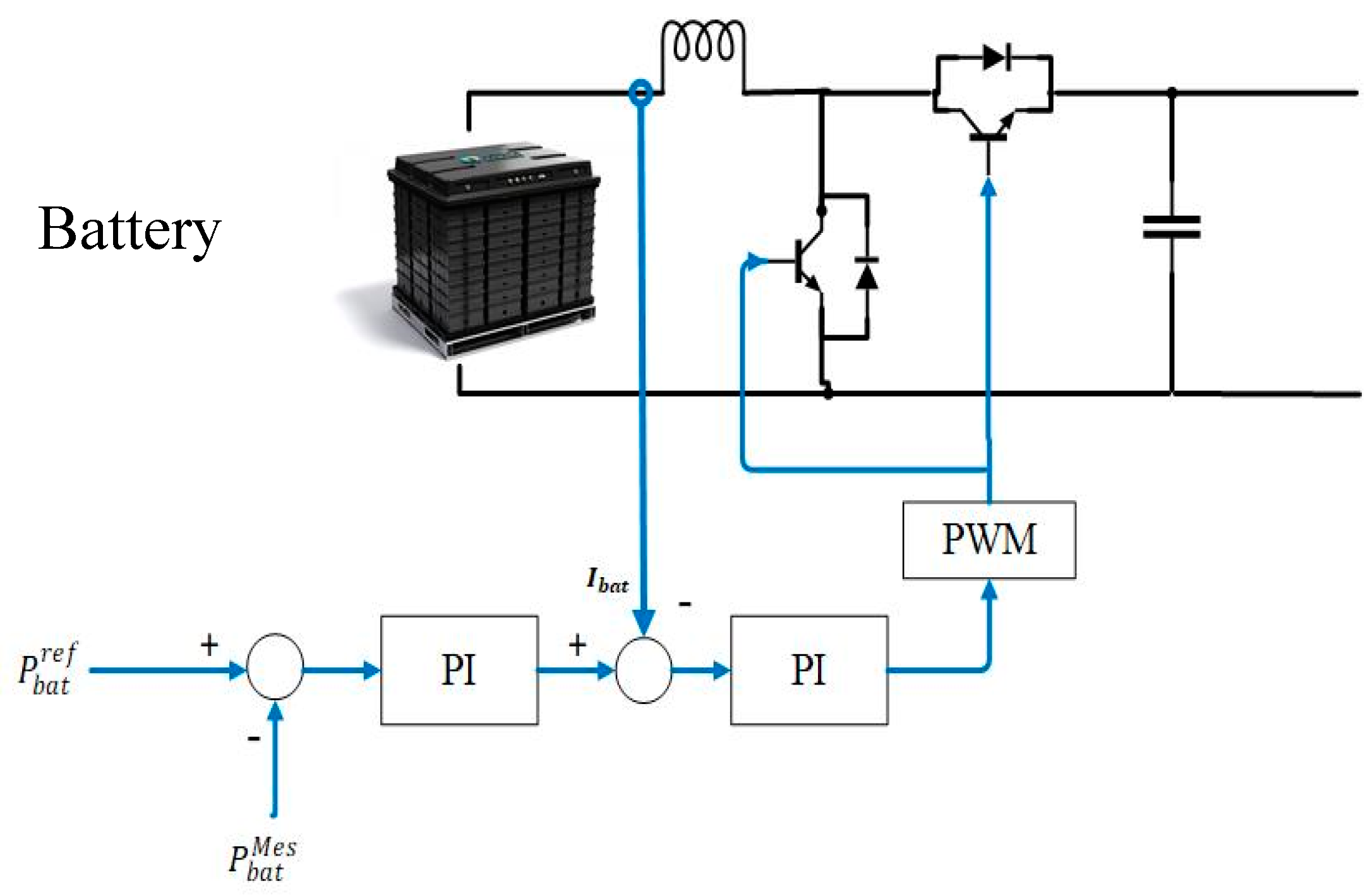
The control design for the ESS’s converter is illustrated in Figure 8. A bidirectional buck/boost converter is designed to control the charging/discharging power of the battery. The converter consists of four switches with a PWM control circuit. When S1 is off and S2 is on, the converter works in buck mode. In this case, power is transferred from the DC bus to charge the battery. On the other hand, when S1 is switched on and S2 switched off, the converter works in boost mode and power is discharged from the battery and transferred to the DC bus. There are two control loops to control the charging/discharging power of the battery. The reference power, which is obtained from the supervisory controller, is regulated by a proportional integrator (PI) controller. A second PI controller is used to regulate the current of the battery to protect the battery.
2.3. Supervisory Controller
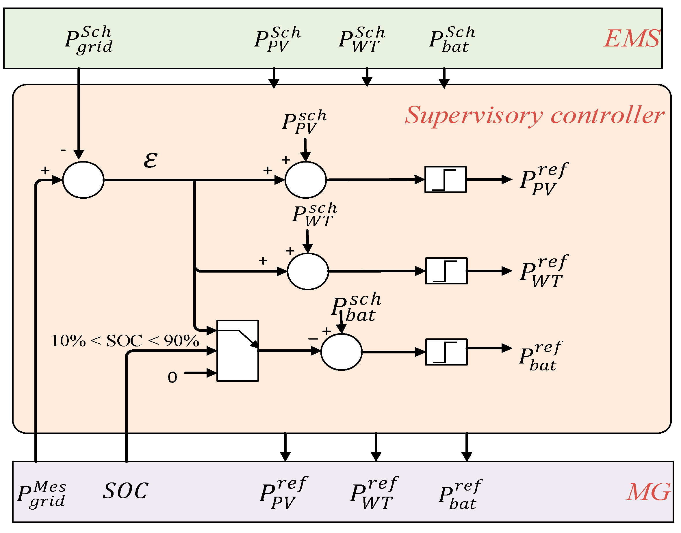
The main purpose of the supervisory controller is to compensate the mismatch between the main power transferred from/to the grid () and scheduled power obtained from EMS (). Therefore, it modifies incremental values () to the scheduled power from the EMS (). Figure 9 shows the schematic diagram of the supervisor control. In non-interactive mode, each RES employs its respective MPPT algorithm, thus the supervisory controller only modifies the reference set point for the battery. On the other hand, in grid-interactive mode, the supervisory controller dictates the reference set points for each RES and ESS.
The input values to the supervisory controller are the scheduled power from the EMS () and the measured values from the MG (). The output values are the reference set points for the MG which are in case of grid-interactive mode and in case of grid non-interactive mode.
The difference between and represents the deviation between the scheduled power and MG power:
When is positive this means that the purchased power from the grid is greater than the scheduled power therefore, the charging of the battery should be minimized and the generated power from each RES should be increased to regulate this increase in the grid power. This error is divided between all RESs and ESS according to the maximum power limit for the RESs and SOC of the battery. If the SOC of the battery exceeds the battery constraints, there will not be any change in the battery reference set point. In this way, the supervisory controller is used to connect EMS with the MG by regulating any mismatch between the scheduled power and the MG power flow by adjusting the reference power of the DERs.
3. Case Study
The selected MG is applied to a variable load which is a real case study of a set of homes located in Oshawa (Ontario, Canada) as shown in Figure 3a. The historical data which is required for forecasting is real data from Ontario’s independent electricity system operator (IESO) [36]. As discussed in the previous section, the proposed MG consists of PV, WT and ESS. The rating and the operational & maintenance cost (O&M) of each RES unit is illustrated in Table 2. Also, the electricity time of use during a typical weekday in the winter season in Oshawa is given in Table 3 [37]. The initial conditions, lower and upper limits of SOC (%) of the battery are set as 50%, 10%, and 90%, respectively.
In this paper, there are two case studies which have been selected to illustrate the objectives of using EMS and supervisory controller in regulating the power flow in economic way. Also, these case studies are prepared with and without the EMS to show the advantage of EMS in saving the operating cost.
3.1. Case 1. Low Demand Profile
In this case, the load demand is less than or equal to the generated power from the DERs of the MG, therefore there is enough power to supply the load. The main grid may sell/purchase power to/from the MG depending on the operating strategy of the system (with or without EMS). Without EMS all the surplus power will be sold to the main grid, but with EMS the MG participates in the open market, purchasing/selling power from/to the utility grid depending on the cost minimization.
3.2. Case 2. High Demand Profile
In this case, the load demand is higher than the generated power from DERs of the MG during some periods of the day. So, the power shortage is supplied from the main grid. The difference between working with or without EMS is the time of purchasing the power and the charging/discharging period of the battery to reduce the operating cost.
4. Results
In this section the results of the proposed system are presented. To ensure the accuracy of the proposed model, the generated power curves for the RESs in the scheduling stage have been determined based on a powerful forecasting tool. Figure 10 presents the generated power profile of PV and WT from the MG and the scheduled power from the EMS. The objectives of the proposed model are presented using these two case studies by comparing the results with and without the EMS.
4.1. Results for Case 1
Figure 11 shows the output results from the proposed MG with and without EMS in the scheduling stage. In addition, it shows the purchased and sold power from/to the main grid during the day.
In the operation without EMS, the demand is supplied from the RESs, and the residual power charges the battery until it reaches its maximum limit. Any surplus power will be sold to the main grid to maintain system stability. Also, if the generated power from the RESs is lower than the load demand, the battery will supply this shortage as shown in Figure 11 (right side). In case of EMS, all the DERs and the main grid are participating in supplying the load, according to an optimization technique. This mean that the MG purchases/sells the power from/to the main grid depending on the cost function as shown in Figure 11 (left side).
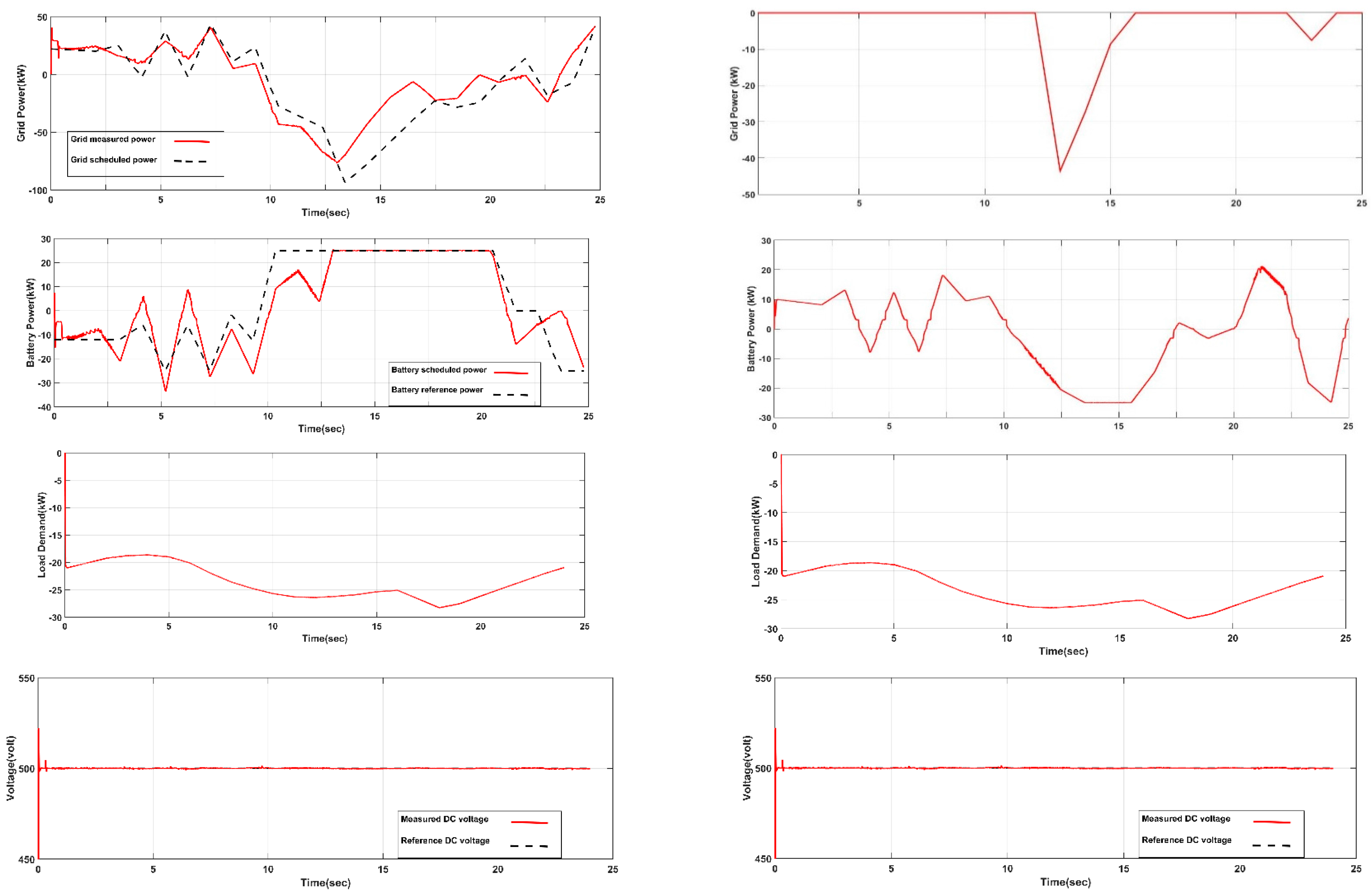
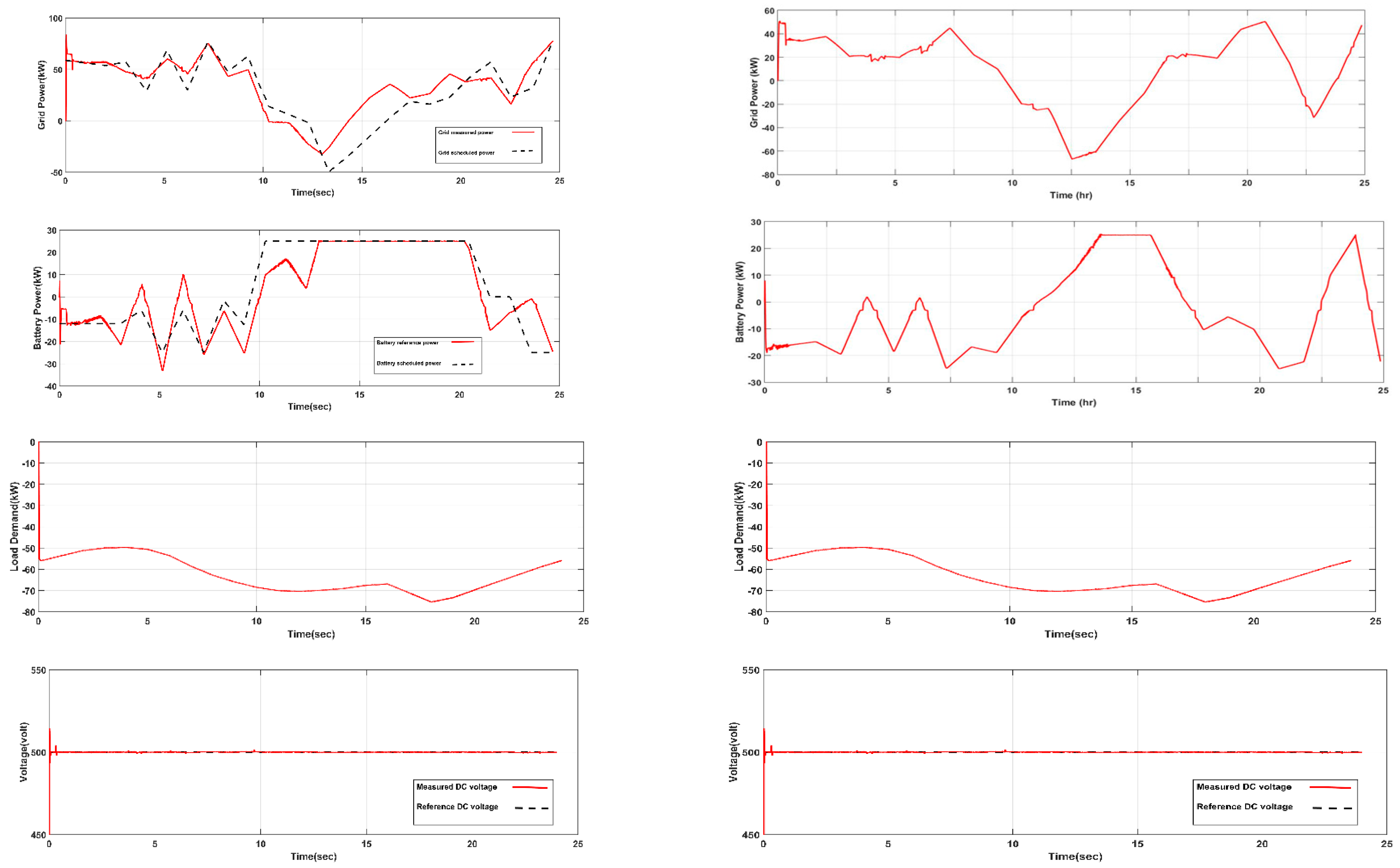
Figure 12 represents the final output results from the proposed MG with and without EMS. In addition to comparing the scheduled power obtained by the EMS and the measured power obtained from the MG system. Curves were arranged as follows: grid power, battery power, load power and DC bus voltage.
The output results obtained by the first strategy (without EMS) are shown in Figure 12 (right side). In the period (00:00–9:00) the demand is higher than the generated power from the RESs, therefore the battery discharges the power to cover this shortage to prevent purchasing power from the grid. From 09:00 to15:00, the RESs generate more power than the load consumption, so the surplus power is stored in the battery until reaching the maximum limit. Any residual power is sold to the grid. In the period (15:00–20:00), the load increased so the power shortage is covered by the battery. Finally, the period from (20:00 to 22:00) and from (22:00 to 23:00) there is a variation on the wind speed, thus a variation in the WT generated power. Therefore, the battery charges and then discharges again to cover the demand. This means that the priority for this strategy is to reduce the amount of power purchased from the grid.
On the other hand, the results obtained by the proposed strategy (with EMS) show that the MG purchases power from the grid during off-peak period (00:00–07:00 and 19:00–23:59) to supply the load and store the generated power from RESs in the battery. During on-peak and medium-peak periods, all the stored power and the surplus power is sold to the grid as shown in Figure 12 (left side). Table 4 shows the operating cost and the electricity trade for both strategies. From the obtained results, the operating cost with the EMS shows the best results.
The results also show the mismatch between the scheduled grid power and MG grid power, as well as the task of supervisory control in adjusting the battery reference power to reduce purchased power from the grid. The obtained results show the power of the local control system in following the reference set points at any time and in regulating the DC bus voltage at a fixed value.
4.2. Results for Case 2
In this case, the demanded load is higher than the generated power of the MG, thus it is required to purchase power from the main grid during some periods of the day. The variable profiles shown in Figure 13 are like the variables used in case 1. Based on the results obtained from the MG with and without EMS, there is a significant difference between the two strategies in purchasing and selling the power from the grid during the day. The purchased power from the grid in the first strategy (without EMS) depends on the load demand, but in the proposed strategy (with EMS) it depends on the electricity price during the day.
The output power from the scheduling stage is presented in Figure 14 with and without EMS. It illustrates the purchased/sold power from/to the main grid during the day. In the first strategy, the MG uses the battery and the RESs to supply the load and any shortage is supplied from the grid. After the SOC of the battery reaches the minimum limit, the battery starts to charge so more power will be purchased from the grid, until battery can be charged from the RESs. Therefore, the MG absorbs power from the grid without taking into consideration the electricity price during the day.
In the proposed strategy (with EMS) the battery is charged by the RESs during low price periods and discharges during the high price periods. This means that the MG purchases more power from the grid during the off-peak periods than the on-peak periods to reduce the operating cost. Also, if there is any surplus of generated power that is not required to serve the load demand, it will be sold to the grid with high price as shown in Figure 13 (left side).
In the same time, the results show the advantages of supervisory controller in adjusting the battery reference set point depending on the mismatch between the measured power from the grid and the grid scheduled power as illustrated in Figure 13. In addition, Figure 13 shows that the DC bus voltage is fixed at a certain value because of the powerful of the local controller. Table 4 gives the electricity trade results for both case studies, with and without EMS, and the advantages of using EMS.
In this way, the EMS uses an optimization method to reduce the operational cost by controlling the charging/discharging periods of the battery to manage the unbalance between the RES generated power and the load demand, based on the electricity price. Also, the results show how the supervisory controller adjusts the mismatch between the main grid power and the grid scheduled power by adjusting the reference set point for the battery in case of non-interactive operation. In case of grid-interactive operation, the supervisory control adjusts the reference set points for both RESs and battery as shown in Figure 9.
5. Conclusions
Using the EMS as part of the control design of a grid-connected microgrid can minimize the total operating cost. The proposed EMS has been implemented to ensure the best management of power for the MG sources based on a powerful heuristic optimization method (ISA). The optimization model is flexible so that different DGs can be added to the MG system. Supervisory control has been added to the control model to adjust any deviation between the main grid power and the scheduled reference power by modifying the reference set-point of the battery power given by the EMS. This paper presents a full local control design for the proposed system. The local controller controls the local power, current and DC voltage of the MG where the purpose of the local controller is to follow the setting point of the supervisor controller. The developed methodology is applied to a real case study of a set of homes located in Oshawa, Ontario, Canada. All the data required such as load demand, weather conditions for the day-ahead scheduling is forecasted using WNN which is not in the scope of this paper. Two cases of operating strategies have been used to verify the objectives of the proposed model. The operation of MG is tested with and without EMS to verify the advantages of using EMS in the control method. The proposed Control design solves the problem that faces the stockholders which is how to design a microgrid in a reliable and economical manner.
Author Contributions
The literature review and manuscript preparation, as well as the simulations, were carried out by Mohamed El-Hendawi. Final review of manuscript corrections was done by Hossam A. Gabbar, Gaber El-Saady and El-Nobi A. Ibrahim.
Conflicts of Interest
The authors declare no conflict of interest.
References
- Khan, M.W.; Wang, J. The research on multi-agent system for microgrid control and optimization. Renew. Sustain. Energy Rev. 2017, 80, 1399–1411. [Google Scholar] [CrossRef]
- Wu, X.; Wang, X.; Member, S.; Qu, C.; Member, S.; Sets, A. A Hierarchical Framework for Generation Scheduling of Microgrids. IEEE Trans. Power Deliv. 2014, 29, 2448–2457. [Google Scholar] [CrossRef]
- Gabbar, H.A.; El-hendawi, M. Supervisory Controller for Power Management of AC/DC Microgrid. In Proceedings of the 2016 IEEE Smart Energy Grid Engineering (SEGE), Oshawa, ON, Canada, 21–24 August 2016; pp. 147–152. [Google Scholar]
- Tummuru, N.R.; Ukil, A.; Gooi, H.B.; Verma, A.K.; Kollimalla, S.K. Energy Management of AC-DC Microgrid under Grid-connected and Islanded Modes. In Proceedings of the IECON 2016—42nd Annual Conference of the IEEE Industrial Electronics Society, Florence, Italy, 23–26 October 2016; pp. 2040–2045. [Google Scholar]
- Sekhar, P.C.; Mishra, S.; Sharma, R. Data analytics based neuro-fuzzy controller for diesel-photovoltaic hybrid AC microgrid. IET Gener. Transm. Distrib. 2015, 9, 193–207. [Google Scholar] [CrossRef]
- Sekhar, P.C.; Mishra, S.; Member, S. Storage Free Smart Energy Management for Frequency Control in a Diesel-PV-Fuel Cell-Based Hybrid AC Microgrid. IEEE Trans. Neural Netw. Learn. Syst. 2016, 27, 1657–1671. [Google Scholar] [CrossRef] [PubMed]
- Kallamadi, M.; Sarkar, V. Enhanced real-time power balancing of an AC microgrid through transiently coupled droop control. IET Gener. Transm. Distrib. 2017, 11, 1933–1942. [Google Scholar] [CrossRef]
- Ma, W.; Wang, J.; Member, S.; Lu, X. Optimal Operation Mode Selection for a DC Microgrid IEEE Trans. Smart Grid. 2016, 7, 2624–2632. [Google Scholar] [CrossRef]
- Dou, C.; Yue, D.; Guerrero, J.M.; Xie, X.; Hu, S. Multiagent System-Based Distributed Coordinated Control for Radial DC Microgrid Considering Transmission Time Delays. IEEE Trans. Smart Grid. 2017, 8, 2370–2381. [Google Scholar] [CrossRef]
- Zhao, X.; Li, Y.W.; Tian, H.; Wu, X. Energy Management Strategy of Multiple Supercapacitors in a DC Microgrid Using. IEEE J. Emerg. Sel. Top. Power Electron. 2016, 4, 1174–1185. [Google Scholar] [CrossRef]
- Ac, H.; Microgrid, D.C.; Xiao, H.; Luo, A.; Member, S.; Shuai, Z. An Improved Control Method for Multiple Bidirectional Power Converters in. IEEE Trans. Power Electron. 2016, 7, 340–347. [Google Scholar]
- Meng, L.; Riva, E.; Luna, A.; Dragicevic, T.; Vasquez, J.C.; Guerrero, J.M. Microgrid supervisory controllers and energy management systems: A literature review. Renew. Sustain. Energy Rev. 2016, 60, 1263–1273. [Google Scholar] [CrossRef]
- Boukettaya, G.; Krichen, L. A dynamic power management strategy of a grid connected hybrid generation system using wind, photovoltaic and Flywheel Energy Storage System in residential applications. Energy 2014, 71, 148–159. [Google Scholar] [CrossRef]
- Liu, X.; Wang, P.; Loh, P.C. A hybrid AC/DC microgrid and its coordination control. IEEE Trans. Smart Grid 2011, 2, 278–286. [Google Scholar]
- Gabbar, H.A. Energy management strategy for AC/DC microgrid Mohamed El-Hendawi Gaber El-Saady and El-Nobi A. Ibrahim. Int. J. Process Syst. Eng. 2017, 4, 169–183. [Google Scholar]
- Hosseinzadeh, M.; Member, S.; Salmasi, F.R.; Member, S. Robust Optimal Power Management System for a Hybrid AC/DC Micro-Grid. IEEE Trans. Sustain. Energy 2015, 6, 675–687. [Google Scholar] [CrossRef]
- Elsied, M.; Oukaour, A.; Gualous, H.; Hassan, R. Energy management and optimization in microgrid system based on green energy. Energy 2015, 84, 139–151. [Google Scholar] [CrossRef]
- Elsied, M.; Oukaour, A.; Gualous, H.; Brutto, O.A.L. Optimal economic and environment operation of micro-grid power systems Loss of Power Supply Probability. Energy Convers. Manag. 2016, 122, 182–194. [Google Scholar] [CrossRef]
- Luna, A.C.; Diaz, N.L.; Graells, M.; Vasquez, J.C.; Guerrero, J.M. Mixed-Integer-Linear-Programming-Based Energy Management System for Hybrid PV-Wind-Battery Experimental Verification. IEEE Trans. Power Electron. 2017, 32, 2769–2783. [Google Scholar] [CrossRef]
- Huang, H.; Member, S.; Cai, Y.; Member, S. A Multiagent Minority-Game-Based Demand-Response Management of Smart Buildings Toward Peak Load Reduction. IEEE Trans. Comput. Des. Integr. Circuits Syst. 2017, 36, 573–585. [Google Scholar] [CrossRef]
- Lyzwa, W.; Member, S.; Wierzbowski, M. MILP Formulation for Energy Mix Optimization. IEEE Trans. Ind. Inform. 2015, 11, 1166–1178. [Google Scholar] [CrossRef]
- Fathima, A.H.; Palanisamy, K. Optimization in microgrids with hybrid energy systems—A review. Renew. Sustain. Energy Rev. 2015, 45, 431–446. [Google Scholar] [CrossRef]
- Rouholamini, M.; Mohammadian, M. Energy management of a grid-tied residential-scale hybrid renewable generation system incorporating fuel cell and electrolyzer. Energy Build. 2015, 102, 406–416. [Google Scholar] [CrossRef]
- Marra, F.; Yang, G.; Træholt, C.; Østergaard, J.; Member, S.; Larsen, E. A Decentralized Storage Strategy for Residential Feeders With Photovoltaics. IEEE Trans. Smart Grid 2014, 5, 974–981. [Google Scholar] [CrossRef] [Green Version]
- Microgrid, A.C.D.C. Overview of PowerManagement Strategies of Hybrid AC/DC Microgrid. IEEE Trans. Power Electron. 2015, 30, 7072–7089. [Google Scholar]
- Modes, I.; Yi, Z.; Member, S.; Dong, W.; Etemadi, A.H. A Unified Control and Power Management Scheme for PV-Battery-Based Hybrid Microgrids for Both. IEEE Trans. Smart Grid 2017, 3053, 1–11. [Google Scholar]
- Moazzami, M.; Khodabakhshian, A.; Hooshmand, R. A new hybrid day-ahead peak load forecasting method for Iran’s National Grid. Appl. Energy 2013, 101, 489–501. [Google Scholar] [CrossRef]
- Khuntia, S.R.; Rueda, J.L.; van der Meijden, M.A.M.M. Forecasting the load of electrical power systems in mid- and long-term horizons: A review. IET Gener. Transm. Distrib. 2016, 10, 3971–3977. [Google Scholar] [CrossRef]
- Baladr, C.; Aguiar, J.M.; Hern, L. Artificial neural networks for short-term load forecasting in microgrids environment. Energy 2014, 75, 252–264. [Google Scholar]
- Rana, M.; Koprinska, I. Neurocomputing Forecasting electricity load with advanced wavelet neural networks. Neurocomputing 2016, 182, 118–132. [Google Scholar] [CrossRef]
- Gandomi, A.H. Interior search algorithm (ISA): A novel approach for global optimization. ISA Trans. 2014, 53, 1168–1183. [Google Scholar] [CrossRef] [PubMed]
- Kumar, M.; Rawat, T.K.; Jain, A.; Singh, A.A.; Mittal, A. Design of Digital Differentiators Using Interior Search Algorithm. Procedia Comput. Sci. 2015, 57, 368–376. [Google Scholar] [CrossRef]
- Rahimi, M. Electrical Power and Energy Systems Modeling, control and stability analysis of grid connected PMSG based wind turbine assisted with diode rectifier and boost converter. Int. J. Electr. Power Energy Syst. 2017, 93, 84–96. [Google Scholar] [CrossRef]
- Errami, Y.; Ouassaid, M.; Maaroufi, M. Control of a PMSG based wind energy generation system for power maximization and grid fault conditions. Energy Procedia 2013, 42, 220–229. [Google Scholar] [CrossRef]
- Ibrahim, E.; El-hendawi, M. Simulated Annealing Modeling and Analog MPPT Simulation for Standalone Photovoltaic Arrays. Int. J. Power Eng. Energy 2013, 4, 353–360. [Google Scholar]
- Ontario’s Independent Electricity System Operator. Available online: http://www.ieso.ca/power-data (accessed on 1 May 2017).
- Ontario Energy Board. Available online: www.oeb.ca/rates-and-your-bill/electricity-rates (accessed on 1 May 2017).
Figure 1.
Basic structure of the proposed microgrid (MG).

Figure 2.
Energy management system (EMS) and control for the proposed MG. WNN: wavelet neural network; ISA: interior search algorithm.
Figure 2.
Energy management system (EMS) and control for the proposed MG. WNN: wavelet neural network; ISA: interior search algorithm.

Figure 3.
The output of the forecasting system. (a) Load demand. (b) Irradiance. (c) Wind speed.

Figure 4.
ISA flowchart.

Figure 5.
Control design of the grid side converter. PWM: pulse width modulation; PLL: phase locked loop.
Figure 5.
Control design of the grid side converter. PWM: pulse width modulation; PLL: phase locked loop.

Figure 6.
Control design for the wind turbine (WT) generator. PMSG: permanent magnet synchronous generator; MPPT: maximum power point tracking.
Figure 6.
Control design for the wind turbine (WT) generator. PMSG: permanent magnet synchronous generator; MPPT: maximum power point tracking.

Figure 7.
Control design for PV system.

Figure 8.
Control design of energy storage system (ESS). PI: Proportional Integrator.

Figure 9.
Supervisory controller design. SOC: state of charge; MG: microgrid.

Figure 10.
(a,b) The scheduled and measured generation profiles for PV and WT, respectively.

Figure 11.
(a,b) Microgrid scheduled power flow with and without EMS respectively in case 1. (c,d) The purchased/sold power from the grid during the day with and without EMS.
Figure 11.
(a,b) Microgrid scheduled power flow with and without EMS respectively in case 1. (c,d) The purchased/sold power from the grid during the day with and without EMS.

Figure 12.
The output variables of the proposed MG with (left side) and without (right side) EMS in case 1.
Figure 12.
The output variables of the proposed MG with (left side) and without (right side) EMS in case 1.

Figure 13.
The output variables of the proposed MG with (left side) and without (right side) EMS in case 2.
Figure 13.
The output variables of the proposed MG with (left side) and without (right side) EMS in case 2.

Figure 14.
(a,b) Microgrid scheduled power flow with and without EMS respectively in case 2. (c,d) The purchased/sold power from the grid during the day with and without EMS.
Figure 14.
(a,b) Microgrid scheduled power flow with and without EMS respectively in case 2. (c,d) The purchased/sold power from the grid during the day with and without EMS.


Table 1.
Parameters and variables of the model. WT: wind turbine; ESS: energy storage systems; PV: photovoltaic.
Table 1.
Parameters and variables of the model. WT: wind turbine; ESS: energy storage systems; PV: photovoltaic.
| Name | Description |
|---|---|
| Photovoltaic Power | |
| WT power | |
| ESS power | |
| Power required by the load | |
| The purchased power from the grid | |
| The sold power to the grid | |
| Maintenance cost of PV | |
| Maintenance cost of WT | |
| Maintenance cost of ESS | |
| Cost of purchasing power from the grid | |
| Cost of selling power to the grid | |
| The state variables | |
| State of charge of the battery | |
| T | Number of time slots (24 h) |
| t | Duration of interval (1 h) |
Table 2.
Parameters of RESs.
| Type | PV | Wind |
|---|---|---|
| Min limit (kW) | 0 | 0 |
| Max limit (kW) | 100 | 60 |
| O&M Cost ($/kW) [2] | 0.01 | 0.01 |
Table 3.
Ontario Electricity Tariff Periods.
| Time of Use (Hour) | Off-Peak 00:00–07:00 | On-Peak 07:00–11:00 | Medium-Peak 11:00–17:00 | On-Peak 17:00–19:00 | Off-Peak 19:00–23:59 |
|---|---|---|---|---|---|
| Purchasing price ($/kWh) | 0.087 | 0.18 | 0.132 | 0.18 | 0.087 |
| Selling price ($/kWh) | 0.0435 | 0.09 | 0.066 | 0.09 | 0.0435 |
Table 4.
Electricity trade results for different case studies with and without EMS.
| Case 1 | Case 2 | |||||||||
|---|---|---|---|---|---|---|---|---|---|---|
| Electricity Trade | Electricity Trade | |||||||||
| Purchased Power | Sold Power | Purchase Cost | Sell Cost | Total Cost | Purchased Power | Sold Power | Purchase Cost | Sell Cost | Total Cost | |
| (kWh) | (kWh) | ($) | ($) | ($) | (kWh) | (kWh) | ($) | ($) | ($) | |
| Main Grid only | 567 | 0 | 73.27 | 0 | 73.27 | 756 | 0 | 97.7 | 0 | 195.4 |
| Without EMS | 0 | 87 | 0 | 5.57 | 0.96 | 880 | 0 | 124.58 | 0 | 130.9 |
| With EMS | 237 | 487.7 | 24.07 | 34.8 | −2.6 | 794.85 | 100.64 | 89.96 | 6.68 | 91.44 |
© 2018 by the authors. Licensee MDPI, Basel, Switzerland. This article is an open access article distributed under the terms and conditions of the Creative Commons Attribution (CC BY) license (http://creativecommons.org/licenses/by/4.0/).
Share and Cite
MDPI and ACS Style
El-Hendawi, M.; Gabbar, H.A.; El-Saady, G.; Ibrahim, E.-N.A. Control and EMS of a Grid-Connected Microgrid with Economical Analysis. Energies 2018, 11, 129. https://doi.org/10.3390/en11010129
AMA Style
El-Hendawi M, Gabbar HA, El-Saady G, Ibrahim E-NA. Control and EMS of a Grid-Connected Microgrid with Economical Analysis. Energies. 2018; 11(1):129. https://doi.org/10.3390/en11010129
Chicago/Turabian StyleEl-Hendawi, Mohamed, Hossam A. Gabbar, Gaber El-Saady, and El-Nobi A. Ibrahim. 2018. "Control and EMS of a Grid-Connected Microgrid with Economical Analysis" Energies 11, no. 1: 129. https://doi.org/10.3390/en11010129
Note that from the first issue of 2016, this journal uses article numbers instead of page numbers. See further details here.