Evaluation of the Internal and Borehole Resistances during Thermal Response Tests and Impact on Ground Heat Exchanger Design †

1
De génie mécanique, École de Technologie Supérieure, Montreal, QC H3C1K3, Canada
2
Centre Eau Terre Environnement, Institut national de la recherche scientifique, Québec City, QC G1K9A9, Canada
*
Author to whom correspondence should be addressed.
†
This Paper Presented at the IGSHPA Technical/Research Conference and Expo, Denver, CO, USA, 14–16 March 2017.
Energies 2018, 11(1), 38; https://doi.org/10.3390/en11010038
Submission received: 16 November 2017
/
Revised: 9 December 2017
/
Accepted: 15 December 2017
/
Published: 25 December 2017
(This article belongs to the Special Issue Geothermal Heating and Cooling)
Abstract
:The main parameters evaluated with a conventional thermal response test (TRT) are the subsurface thermal conductivity surrounding the borehole and the effective borehole thermal resistance, when averaging the inlet and outlet temperature of a ground heat exchanger with the arithmetic mean. This effective resistance depends on two resistances: the 2D borehole resistance (Rb) and the 2D internal resistance (Ra) which is associated to the short-circuit effect between pipes in the borehole. This paper presents a field method to evaluate these two components separately. Two approaches are proposed. In the first case, the temperature at the bottom of the borehole is measured at the same time as the inlet and outlet temperatures as done in a conventional TRT. In the second case, different flow rates are used during the experiment to infer the internal resistance. Both approaches assumed a predefined temperature profile inside the borehole. The methods were applied to real experimental tests and compared with numerical simulations. Interesting results were found by comparison with theoretical resistances calculated with the multipole method. The motivation for this work is evidenced by analyzing the impact of the internal resistance on a typical geothermal system design. It is shown to be important to know both resistance components to predict the variation of the effective resistance when the flow rate and the height of the boreholes are changed during the design process.
1. Introduction
Conventional thermal response tests (TRTs), successfully implemented in the commercial geothermal sector, involve injecting a heat pulse into a borehole and measuring its temperature response [1]. Heat is commonly generated by an electrical resistance outside the borehole and transported through a heat carrier fluid, usually water flowing inside the borehole. Heat can also be generated using a heating cable inside the borehole [2]. Heat pumps have alternatively been used with heated or cooled water circulating in a pilot ground heat exchanger (GHE) [3]. The method is mostly used to evaluate the subsurface thermal conductivity when designing ground-coupled heat pump (GCHP) systems but an evaluation of the borehole resistance can also be provided during the test. This last parameter is characteristic of the borehole heat transfer performances and can be assessed for quality control purposes [4]. These two parameters are related to the mean fluid temperature inside the borehole. However the definition of this temperature is not unique. A simple definition is to take the arithmetic mean between the inlet and outlet temperature defined as:
Using this definition, the resistance inferred from the test represents an effective resistance [5] defined in the next section. This resistance has been introduced by Hellström [6] and is dependent on two resistances: the 2D borehole resistance (Rb) and the 2D internal resistance (Ra). Its definition is also not unique since it depends on how the heat transfer varies along the borehole. In order to better predict the 2D resistance Rb, Marcotte and Pasquier [7] proposed to use a different expression for the fluid temperature called p-linear average defined as:
where To is the undisturbed ground temperature and ΔT = T − To. They proposed to use Equation (2), with p → −1. Beier [8], using an analytical modeling approach, found that the use of the p-linear average, although not exact gives less error for the evaluation of the borehole resistance. Beier and Spitler [9] proposed to use a weighted average temperature defined as:
where f, is a time-dependent weighting factor which depends on several factors including the borehole resistance, the flow rate and the borehole height.
The objective of this paper is to present field procedures to evaluate both resistances (Rb) and (Ra) during a thermal response test. To our knowledge, this has not been proposed before. Two methods are described and verified: in the first case, the temperature at the bottom of the borehole is measured at the same time as the inlet and outlet temperatures as done in a conventional TRT and in the second case, the two components of resistances are inferred using different flow rates during the test. The methods are based on an assumed temperature profile inside the borehole. Two profiles are used: the first one is based on assuming a uniform borehole temperature proposed initially by Hellström [6] and the second one suggested by Beier [8] where the assumption of uniform borehole temperature is removed.
2. Theoretical Background
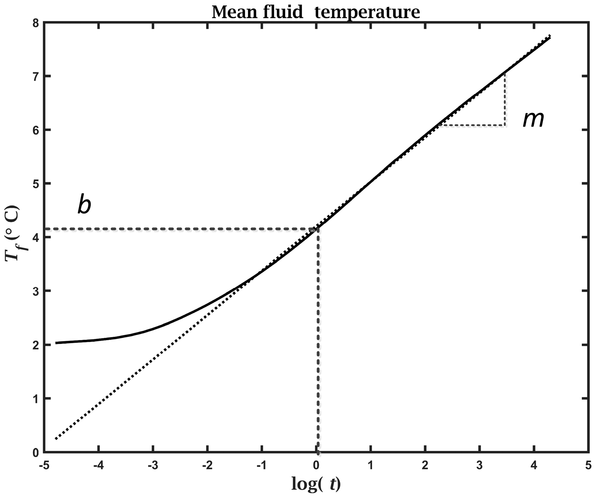
The most common and basic method to evaluate the subsurface thermal conductivity from a TRT is called the slope method [10]. The mean temperature is plotted with respect to the logarithm of the time and the thermal conductivity is related to the slope of the curve. This formula comes from the well-known expression of the infinite line source [11]. Indeed, if we assume that the heat is released at the origin of the borehole and that it depends only on the radial conduction, which is a valid approximation for the time scale of a TRT, the mean fluid temperature is given by:
where E1 is the exponential integral, q’inj is the amount of heat per meter injected during the test, Rb is the borehole resistance and Fo is the Fourier number based on the borehole radius. This expression is only valid for Fourier numbers larger than 5. For these values, it is known that the exponential integral is proportional to the natural logarithm of time. It follows that:
where m is the slope and b is the intercept of the linear approximation (Figure 1).
Raymond et al. [12] have suggested separating the TRT in two parts: an injection period similar to the conventional method followed by a monitoring of the thermal recovery period where no heat is injected. Since the temperature becomes independent of the borehole resistance during the thermal recovery, it is suggested to use this period to evaluate the thermal conductivity and the heat injection period to evaluate the borehole thermal resistance. Austin et al. [13] used optimization methods to evaluate the unknown parameters using a parameter estimation algorithm. Whatever method is used, the definition of the average fluid temperature in Equation (4) have an influence in the estimated borehole resistance. As stated in the introduction, if the arithmetic mean is used like in Equation (1), the value given by Equation (5) for the borehole resistance will be closed to the effective borehole resistance.
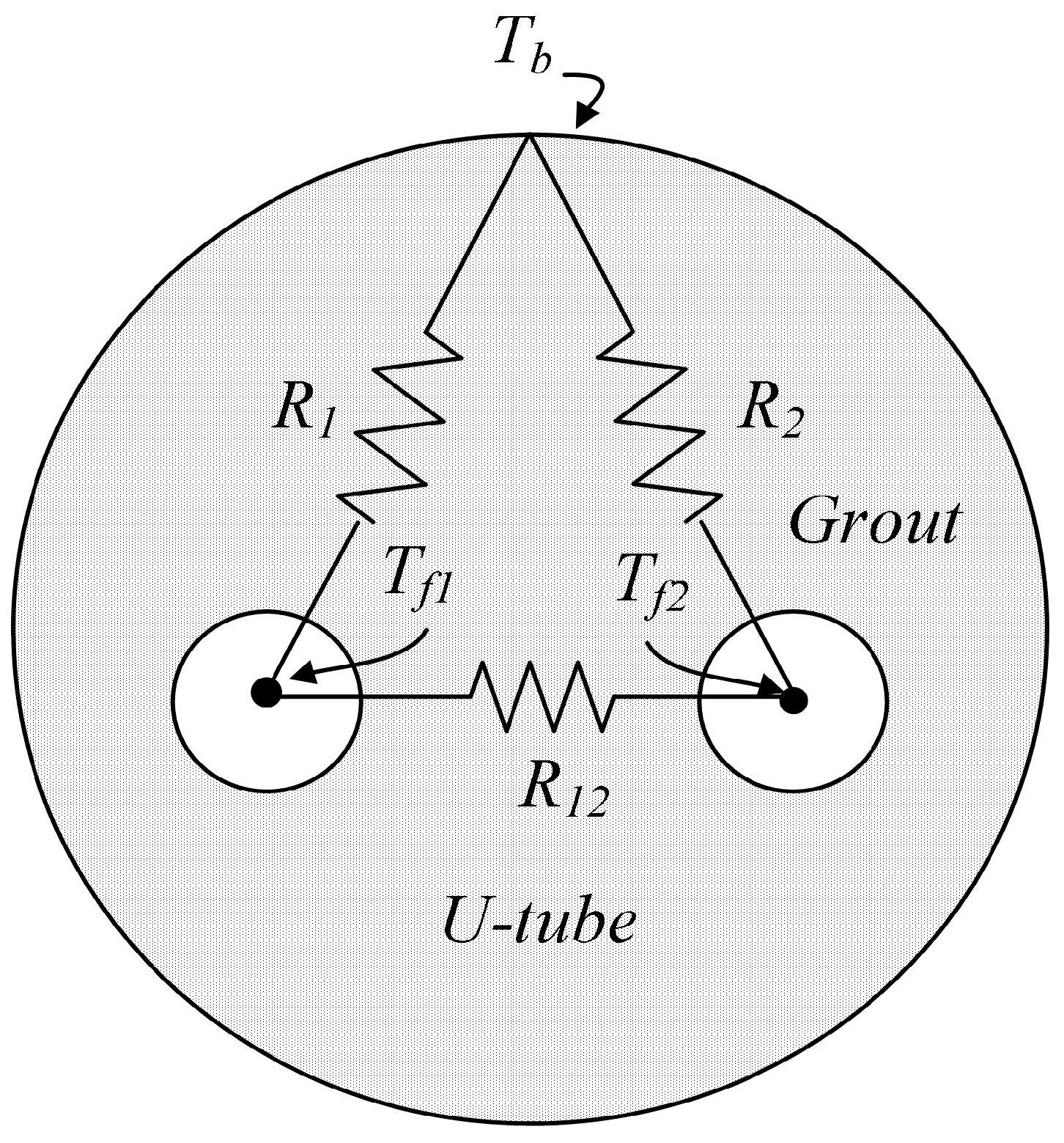
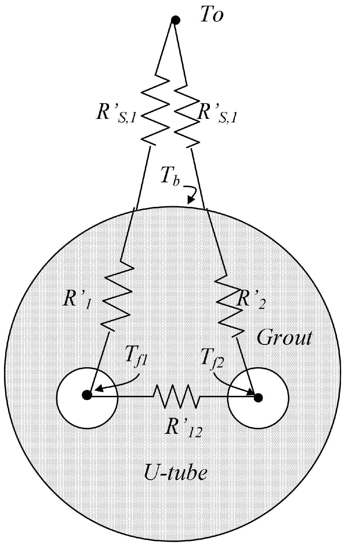
The concept of the effective borehole resistance was introduced by Hellström [6] and is greater than the borehole resistance because the former takes into account the loss of performance due to the short-circuiting effect between the two segments of the U-tube inside the borehole. It is associated with the 2D resistance network inside the borehole. This network is shown in Figure 2 which represents a cross section of a typical borehole with a single U-tube.
The borehole resistance Rb is found by taking the resistances R1 and R2 in parallel and the internal resistance is given by evaluating the equivalent resistance between both legs. In the symmetrical case (R1 = R2), it gives:
From the resistance network, it is easy to see that the heat transfer per unit length is given by:
Hellström [6] found that, if the borehole temperature (Tb) is uniform along the borehole, the temperature distribution inside the borehole can be evaluated by the expressions:
for the downward portion of the pipe and:
for the upward pipe portion. The different parameters are defined as:
It can be observed that, although the fluid and borehole temperatures vary with time, the reduced temperature variation (θ) is assumed to be time independent. This is however only true in the steady-flux regime which represents few hours in a typical borehole. From that distribution, Hellström found that the heat transfer per unit length can now be expressed by a similar expression than Equation (7):
where the new resistance was called the effective borehole and is given by:
If the heat transfer per unit length was assumed to be the same along the borehole, Hellström found that:
In practice, neither of the assumptions are strictly valid, but most of the time they give a good approximation of the internal heat transfer in real boreholes.
The concept of effective resistance was extended to double U-tubes arrangements by Zeng et al. [14]. Only this effective resistance is needed to evaluate the total length of the bore field in a typical design. However, if the parameters between the TRT and the real Ground Coupled Heat Pump GCHP system vary, like the depth of the borehole, it would be important to evaluate both resistances (Ra and Rb) in a TRT to adjust design parameters according to the field response. Lamarche et al. [15] proposed a method to evaluate these two resistances with a conventional TRT and presented measurements that were conducted in an in-situ test. The method is described with more details in this paper including new numerical simulations to evaluate its applicability.
3. Temperature Measurement at the Bottom of the GHE
A measurement of a temperature profile along the GHE pipe is of great interest in order to have a better understanding of the heat transfer inside the borehole. Measurements of such temperature profile during TRTs were performed by Fujii et al. [16] and Acuña et al. [17] using fiber optic sensors. Unfortunately, the apparatus to evaluate temperature with optical fiber is expensive. Lamarche et al. [5] suggested an approach that can be used to evaluate these resistances assuming the Hellström profile of Equations (8) and (9). The expressions of the given profile at the bottom and at the exit are given by:
Equations (14) and (15) can be solved for the two unknown Rb and Ra with temperature measurement at the bottom of the GHE to infer θbottom and θout. The method was verified using numerical simulations while first results obtained with a real TRT are presented here.
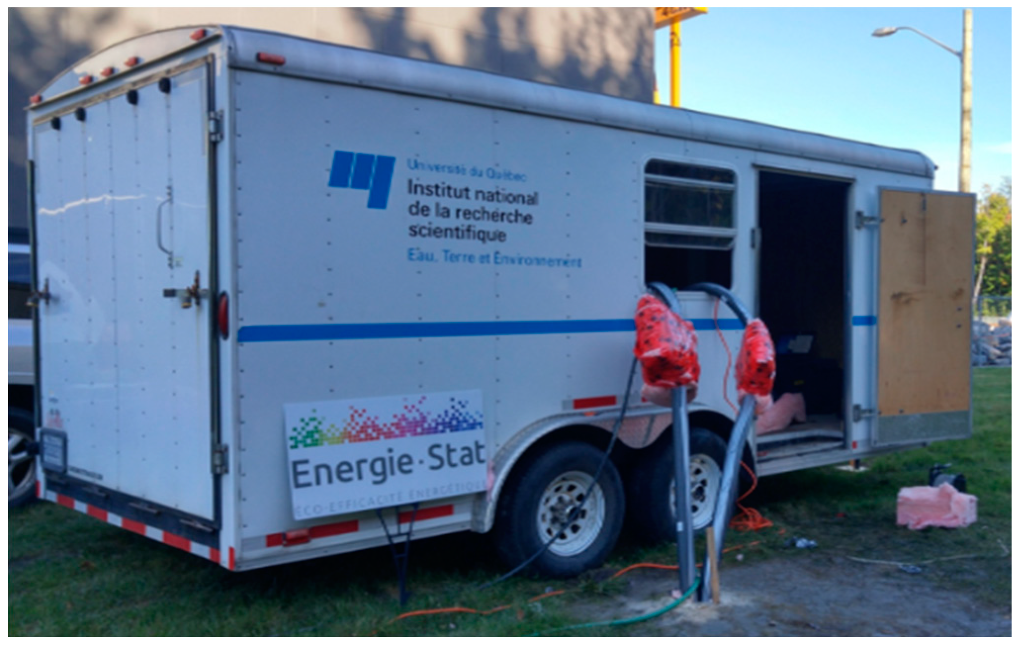
A test was performed at the Institut national de recherche scientifique (INRS) laboratory facilities located in Québec City [18]. The borehole was drilled in 10 m of unconsolidated till and clay followed by 144 m of shale from the Sainte-Rosalie Formation in the St. Lawrence Lowlands geological province (Figure 3). A single U-pipe with no space clips was installed in the borehole filled with thermally enhanced grout. The grout was a mixture of Barotherm® Gold bentonite and silica sand.
Heat injection during the TRT was achieved for 81 h followed by 75 h of thermal recovery monitoring, where heat injection was stopped but water kept circulating in the GHE. The undisturbed subsurface temperature was measured before the test with a submersible probe lowered in the GHE and was 7.9 °C. Table 1 summarizes the other test parameters. Three temperature measurements in the descending pipe leg at depth of 50 m, 100 m and 150 m were carried out with submersible temperature data loggers during the TRT. The average heat injection rate was 62.7 W/m, creating a temperature difference of more than 7 °C between the inlet and outlet of the GHE. The average fluid temperature increased by up to ~20 °C at the end of the test.
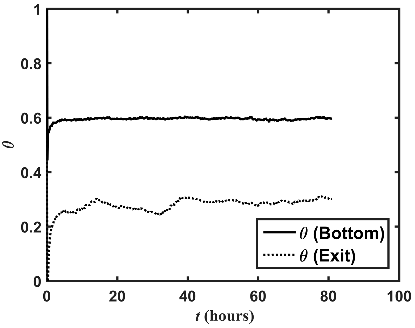
A value of the borehole temperature Tb (t) is needed to solve Equations (10) and (11). This means borehole temperature is not easy to measure. Here, it was estimated using the infinite line source solution from Equation (1) using the subsurface thermal conductivity found during the TRT. Even though the fluid and the borehole temperature are time dependent, in theory, Equations (10) and (11), if valid, should be time independent. To verify that, the measured value of the normalized fluid temperature at the bottom and at the exit were plotted as function of time (Figure 4).
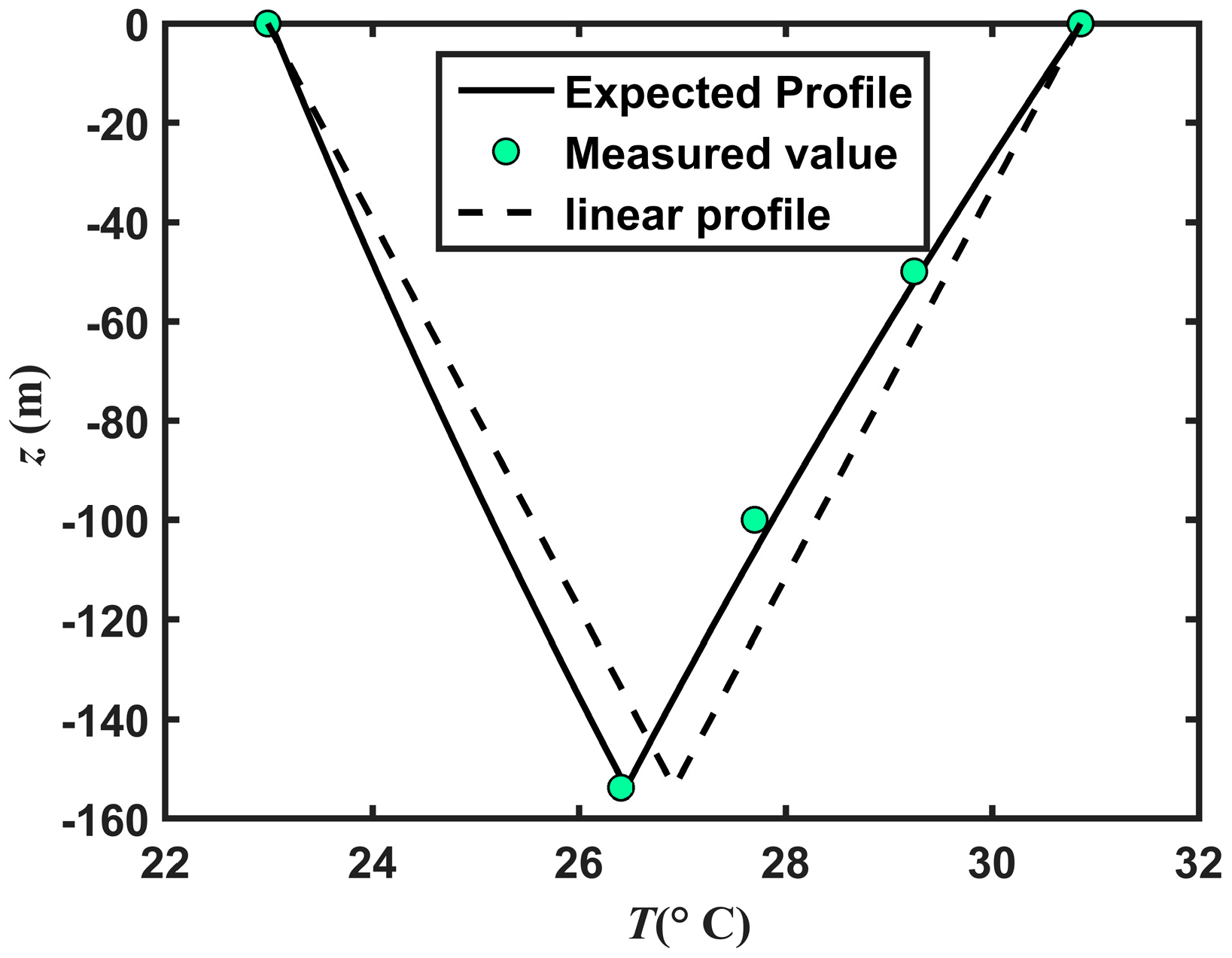
The value became almost constant after approximately 7 h which gives a Fourier number of approximately 6, and is a typical value for the validity of steady-flux regime. In our calculations, the mean measured value of the normalized fluid temperature during the steady-flux regime was used in Equations (14) and (15) in order to find Ra and Rb (Table 2). Results are compared with the calculated resistances using the multipole method [19]. The expected normalized temperature profile is determined using the calculated resistances and compared to the linear profile assuming no thermal short-circuiting between the pipes (Figure 5). Fluid temperature in the descending pipe at 0 m, 50 m, 100 m and 150 m as well as temperature at 0 m in the ascending pipe are superimposed to the expected normalized temperature in the steady-flux regime to evaluate the validity of the method.
Beier Profile
Beier [8] proposed a modified equation to calculate the temperature profile inside the U-tube by coupling the borehole resistance network to the undisturbed ground temperature. He latter developed a modified version taking into account the variation of the ground temperature but, in this manuscript, only the uniform temperature case with symmetric configuration (R1 = R2) was considered. The modified temperature profile is normalized with the ground temperature (Figure 6):
The mathematical expressions for C1, C2, C3, C4, a1, a2, a3 and a4 are described by Beier [8]. They depend on two unknowns (R1 and R12) and known values of the fluid heat capacity, the borehole length and the ground resistance Rs,1 = 2Rs, with Rs given by Equation (4). Expressing Equation (16) and (17) at the bottom and the exit will, in theory, give us the two equations for the two unknowns. One of the advantages of the Beier’s profile is that it is not based on a vertically uniform borehole temperature, an assumption that has been the subject of debates [7,8]. However, one of the disadvantages is that the normalized temperature profile found with Equations (16) and (17) is not time independent, even in the steady-flux regime. The short-circuiting effect in the delta equivalent circuit between both legs of the U-tube will follow two possible paths, a direct one through R12 and an indirect one via the borehole wall temperature Tb (Figure 2). The equivalent resistance found is the internal resistance Ra. In Beir’s model, after a long period of time, the only thermal path between both legs is the resistance R12 and this resistance should then be compared to Ra in the delta circuit and not to R12. However for very small values of time, the borehole temperature is near the soil temperature and the subsurface resistance is small such that the R12 resistance is almost the same as the one in the Delta formalism.
The equations must be solved with temperature measured at a given time to find the borehole resistance network. This practice can introduce errors since measurements are known to vary randomly and averaged values are always a better approach, when possible. It was observed in practice that using temperature at different time in solving Equations (16) and (17), gave large variations in values of R1 and R12. One could, of course, average the thermal resistances found. Instead, the approach used here was not to solve Equations (16) and (17) at a given time but to minimize with a Nelder-Mead algorithm, where the least-square error is defined by:
From these thermal resistance results (Table 3), the expected normalized temperature profile given by Equations (16) and (17) is compared with the measured temperature values (Figure 7). As noted previously, normalized fluid temperatures are time dependent and the absolute temperatures are given for a specific time.
The expected profile matches the experimental data (Figure 7) even though the thermal resistances are different (Table 3). It is important to note that using resistances in Table 2 with the Beier’s profile or the resistances given in Table 3 with the Hellström’s profile will give a wrong normalized temperature profile. Comparing Table 2 and Table 3, we should remember that Rb in the delta model corresponds to R1/2 and Ra to R12 when the tube placement is symmetric. So, it is observed that the borehole resistance gives similar final values but the short-circuit resistances show larger variations. It should be remembered that during this test the interference was small. Any values of the short-circuit resistances will consequently have a small effect on the final results as long as the resistances are large. Also, it should be remembered that the multi-pole evaluation is based on a symmetric configuration, which is not necessarily the case in for real field tests.
4. Resistance Evaluation Using Varying Flow Rate
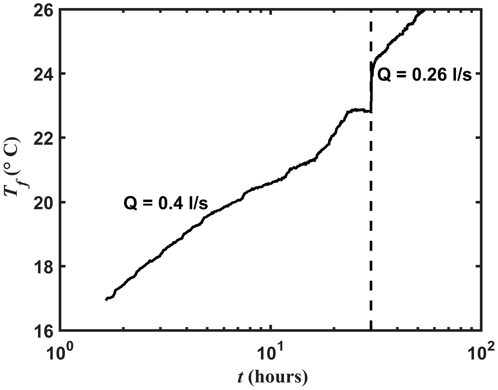
Expressions commonly used by practitioners for the borehole resistance are almost independent on the fluid flow rate. The variation of the flow rate changes the convective resistance but, in turbulent regime, this resistance is very small and from Equation (5), it should be expected that the Intercept of the slope should not change with the flow rate. In practice it is not the case (Figure 8).
The mean fluid temperature is given with respect to time in Figure 8 for a conventional TRT where the flow rate was changed after 30 h of operation. The heat injection rate was kept constant. The change in intercept is not surprising since, according to Lamarche et al. [5], the resistance inferred during a TRT is the effective resistance and not the 2D resistance associated only to the borehole arrangement.
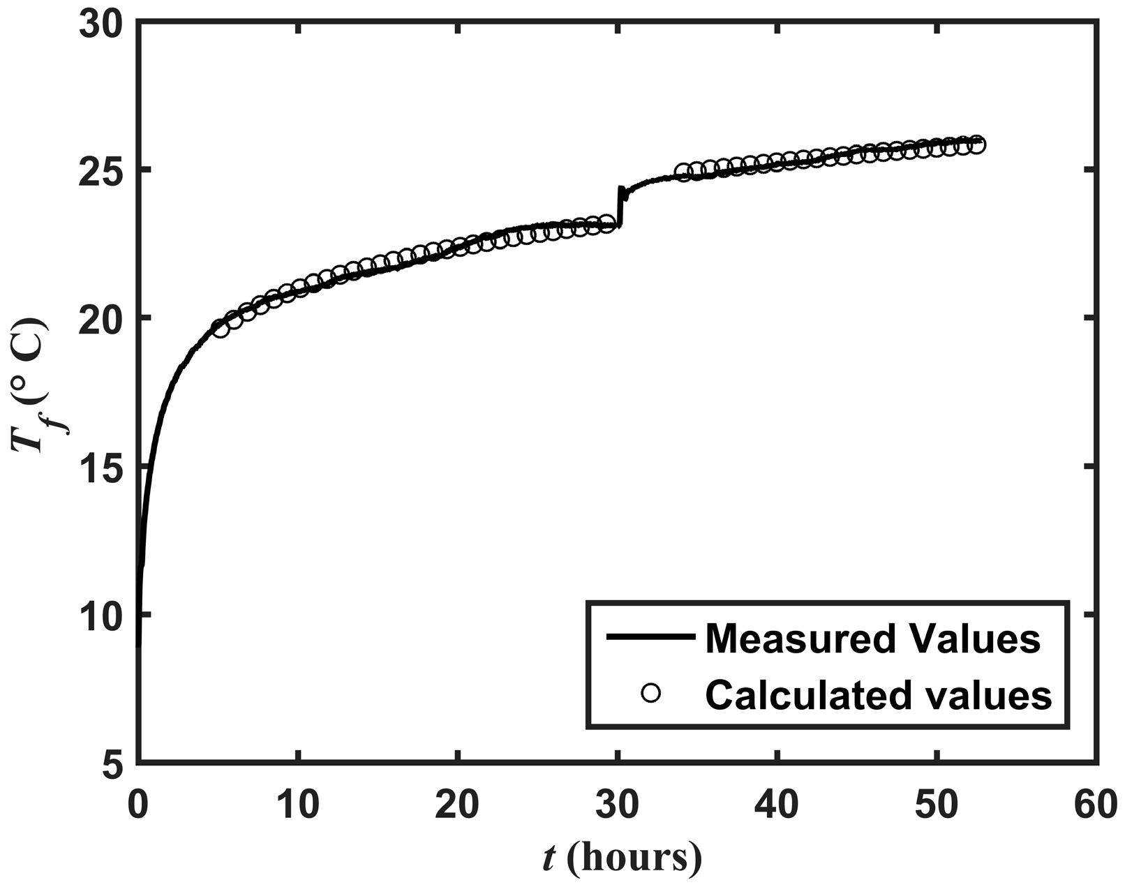
It is clear from Equations (10) and (12) that an increase of the flow rate lowers the effective resistance, which can also decrease if the flow rate diminishes like in Figure 8. A test with variable flow rate was conducted with the same experimental set-up as that presented in the last section. The second test was done three weeks after the end of the first test for the ground temperature to return to its initial condition [18]. The test parameters are the same as those given in Table 1. The heat injection rate was slightly smaller with a mean value of 54 W/m. The flow rate was set at 0.41 l/s for the first 30 h followed by a 23 h period where it was reduced to 0.26 l/s. The Reynolds number during the first part of the test was in the order 18,000, leading to a turbulent flow with a convection resistance of 0.004 mK/W. The flow regime during the second part of the test was still turbulent with a Reynolds number of 11,400 and a convection resistance of 0.003 mK/W. The impact of this convective resistance variation on the total resistance represents a 1% change, which is expected to be smaller than the accuracy at which this parameter can be evaluated. It was, in fact, observed that applying the slope method during data analysis resulted in unrealistic values for the effective borehole resistance. The intercept value from the linear regression in the second part of the variable flow rate test was too sensitive when compared to the noise of the temperature signal. The parameter estimation method was used for the analysis [12]. The same subsurface thermal conductivity as that found in the first TRT was used and only the effective borehole resistance was evaluated. The temperature evolution during the multi-flow test and the one calculated with the borehole parameters found from curve fitting are shown in Figure 9.
The following system of equations was solved from the two values of the estimated effective borehole and internal resistances:
and the corresponding boreholes resistances thus found are given in Table 4.
The analysis reveals a borehole resistance Rb on the same order of magnitude as previously obtained but the internal resistance is smaller (Table 4).
5. Numerical Simulation
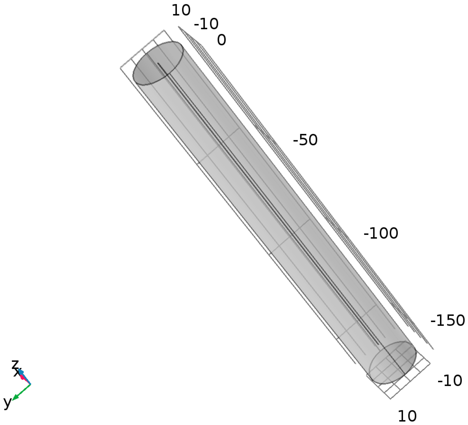
Discrepancies were observed in the first experimental tests between the inferred internal resistance and the ones calculated from the multipole method. A possible explanation is that small variations of the measured temperature can lead to large variations of the internal resistance, especially when the interference effect is small or the short-circuiting resistance is large. A 3D GHE simulation was done with Comsol Multiphysics® 5.2a (COMSOL, Inc., Burlington, MA, USA, www.comsol.com) to provide more insight on the influence of these parameters. The 153 m long borehole was modeled with the Pipe Flow™ module. This module simulates a 1D fully developed flow inside a pipe. The grout region was modeled with a cylindrical solid with known thermal conductivity, whereas the infinite subsurface region was modeled by a finite cylinder of 10 m radius (Figure 10). The effect of the finite region was assumed to be negligible for the short period of time represented by the thermal response test (96 h).
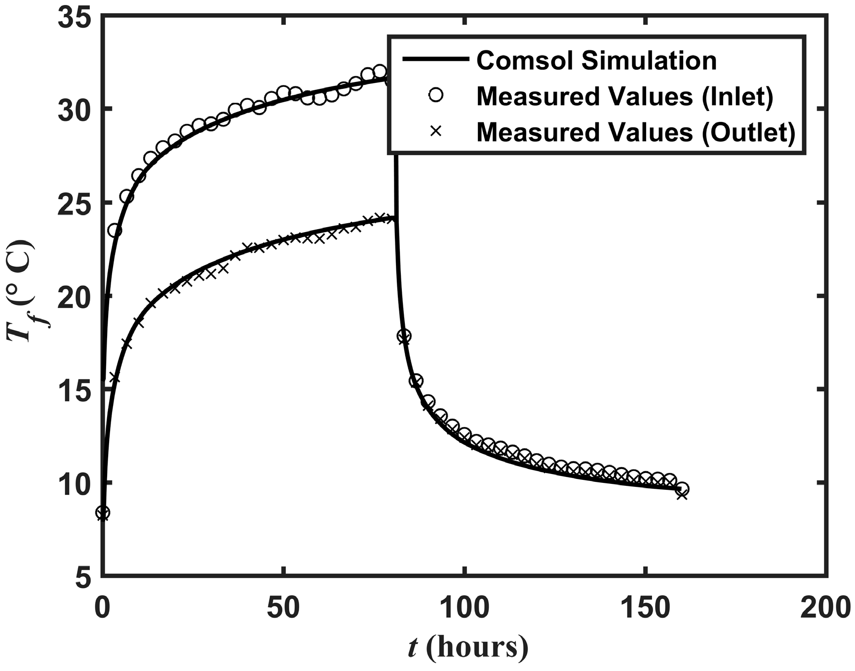
The mesh was refined until no significant variations were observed. The final mesh involved 70,431 elements. The borehole parameters presented in Table 1 were used for the first the numerical simulation. Both the injection and recovery were simulated for the first TRT case. This case was used as a validation of the numerical model. Simulated inlet and outlet temperatures are shown in Figure 11, indicating good agreement between the simulation and the experimental measurements.
The temperature simulated at the bottom of the borehole is additionally compared to that measured during the first TRT (Figure 12), indicating a noticeable discrepancy. The internal resistance was evaluated with the numerical temperature solution using the same procedure as described in Section 3 (Table 5). The internal resistance is different than previous results of Section 2 and more similar to the expected resistance from the multipole method, although the simulated and measured fluid temperatures at the inlet and outlet are almost identical. However, the effective resistance remains similar when compared to results inferred from field data and numerical simulations.
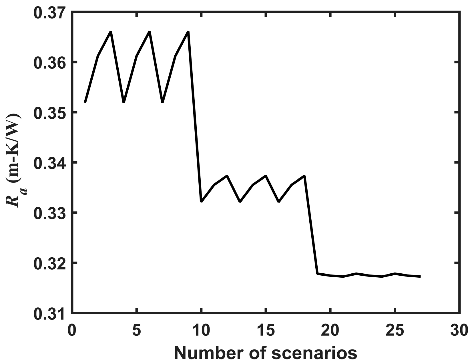
It is known that parameter estimation during a thermal response test is very sensitive to the accuracy of assumed parameters [20,21]. Some of which are geometric, like the borehole radius and the shank spacing, while others can be associated to the physical properties, like the thermal conductivity of the grout. A sensitivity analysis was consequently carried out by varying some of these parameters in order to evaluate if the difference between the internal resistance inferred from measurements and calculated from the multipole method can be explained by such uncertainties. The parameters changed (Table 6) represent a ±20% variation around the nominal TRT values (Table 1).
This results in 27 different combinations from which the internal resistance was calculated using the multipole method (Figure 13).
Variations in internal resistance are large (±20%), but cannot explain the difference between the theoretical and the inferred resistances from the experiment. A possible explanation is a drift of temperature due to sensor accuracy for temperature measured inside the borehole. The downhole sensors were less accurate than the one used for the inlet and outlet temperature measurements. Verification was done using the same measurements as before for the inlet and outlet temperatures (Figure 11 and Figure 12), but lowering all downhole temperature sensors by a value of 0.4 °C. The inferred resistances show a better concordance (Table 7). Although this explanation cannot be confirmed, it most plausible and will have to be validated with further studies.
Virtual Borehole
Using our validated numerical model, the borehole parameters were modified to simulate a case where the thermal interference is expected to play a larger role. This can be the case if the borehole is long or if the flow rate is low. The second approach was adopted for the following simulation. The previous parameters were kept constant except that the flow rate was smaller. The pipe was also smaller to insure a sufficient Reynolds number and maintain a turbulent flow.
The virtual TRT with parameters of Table 8 was analyzed with the method described in Section 3. The outcome of the virtual TRT analysis gave an effective resistance inferred from inlet and outlet temperatures with Equation (5) (1st column; Table 9). The improved TRT analysis with the evaluation of the bottom temperature also gave the internal and borehole resistance from the method of Section 3 and from which the effective resistance is calculated with Equation (12) (4th column; Table 9). Finally a comparison with the multipole method is achieved.
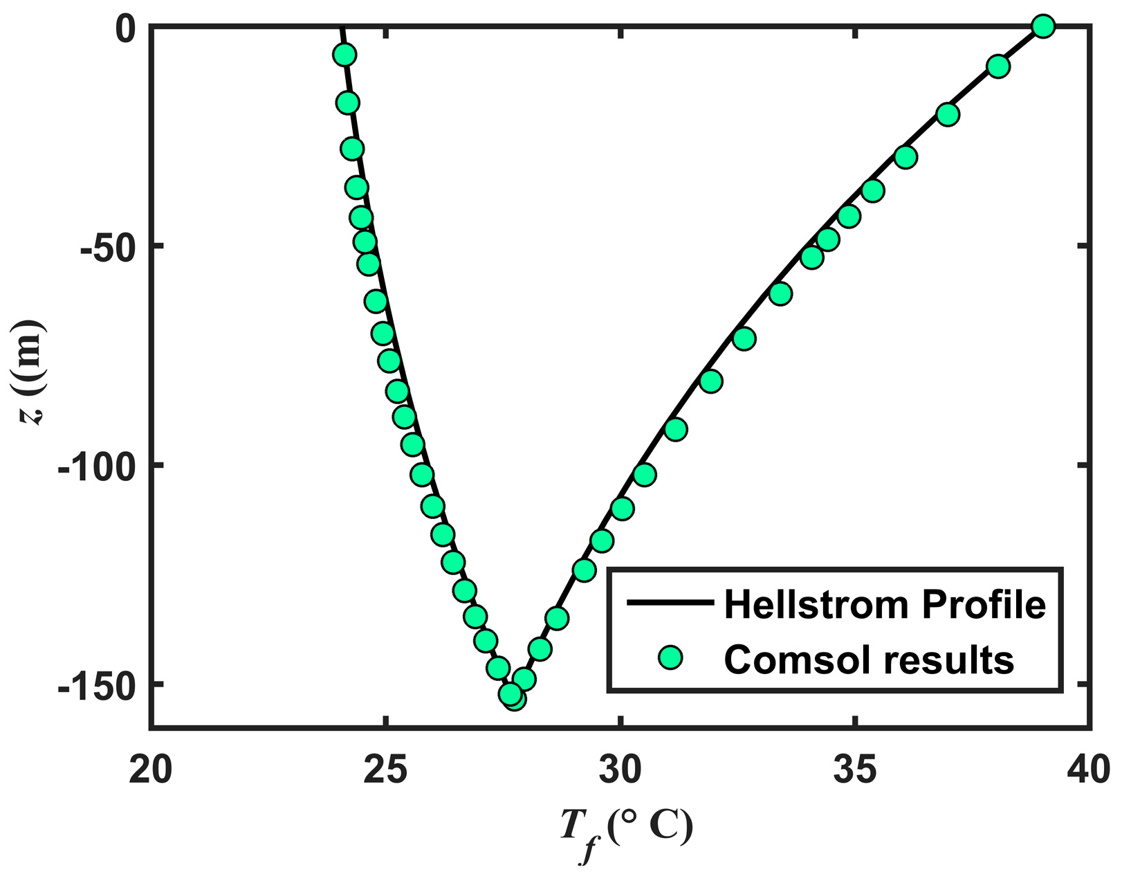
Table 9 reveals that there is a pronounced difference between the borehole resistance Rb and the effective resistance found with the slope method. The expected temperature profile was calculated with Hellström’s approach [6], using the Ra and Rb values obtained with the simulated bottom temperature, and compared with the simulated fluid temperature. This comparison is done for a specific time of simulation, just before the end of the injection period. The results shown in Figure 14 indicate again a very good agreement between the two profiles even though the first one is found assuming a uniform temperature which was already noticed by the first author [5].
6. Impact on a Typical GCHP Design
The knowledge of the internal resistance is believed important and a simple sizing exercise was done to illustrate its impact on GCHP design using the results given in the last section. The simple ASHRAE method [22] was used to size the bore field. The method is based on the following formula:
where Rs is the soil transient resistance for different heat pulses [22]. The three thermal loads associated with annual, monthly and hourly pulses for a typical heating dominated problem were used and are given in Table 10.
The interference between boreholes is neglected (Tp ≈ 0) and the ΔT at the denominator was set at 10 °C for the sake of simplification. The final length given by Equation (17) depends on the borehole thermal resistance. Different values are possible. A borehole resistance calculated according to design criteria with a method proposed in the literature can be used if no TRT is done. The value would be on the order of the Rb calculated with the mutipole method in Table 9 (Rb = 0.134 mK/W), if a 2D approach is chosen and the method does not take into account the short-circuiting between pipes. The designer can alternatively use the 3D effective resistance if the multipole method is considered and the internal resistance is calculated, which would result in = 0.170 mK/W for conditions of Table 8. A TRT experiment, with the slope method, could be considered if there is uncertainty about the borehole properties (grout thermal conductivity, shank spacing, etc.) and would give Rb = 0.165 mK/W (Table 9). This value is, of course, is similar to that of the multipole method since, in the presented numerical simulation, the borehole parameters are exact. Finally, if an improved TRT analysis as described in Section 3 is performed, the Ra and Rb values given in the 2nd and 3rd columns of Table 9 can use in the design with the inferred or calculated effective resistances (1st and 4th columns), which, of course, are almost the same. This can be interesting if, for some reason, the boreholes that will be installed for the complete bore field have a different length or flow rate than the one use for the TRT experiment. Different sizing scenarios were explored in Table 11, where the impact on the total bore length is illustrated with variations of the total borehole length and flow rate affecting the internal resistance. A total length of 2169 m is obtained for the first case that would be repeated if the internal resistance is not assessed from the TRT or neglected in the calculations. Changes in length or flow rate is then shown to potentially undersizing or oversizing the bore field by an order of 10%, at least for the example provided.
7. Discussion and Conclusions
The analysis methods used for the evaluation of the subsurface thermal conductivity during TRTs have become mature. However, some questions remain when considering the evaluation of the borehole thermal resistance. Preliminary work to find both, the borehole resistance and the internal resistance, using the bottom fluid temperature and by varying the flow rate was presented in this manuscript. It was found that the resistances are dependent of the assumed temperature profile along the GHE pipe. The method to estimate the profile should be compatible with the design algorithm to size the bore field when specifying the measured resistances. The approaches suggested by Hellström [6] and Beier [8] were used to evaluate the temperature profile for the TRT and compared with numerical simulations. Both approaches used in this study gave satisfying results, even though the internal resistance was different than expected theoretically. It was observed that the method using the temperature at the bottom is very sensitive to the accuracy of the temperature sensors. Further studies have to be done to see if this can be a possible handicap of the method. Numerical calculations, simulating a TRT with higher internal thermal interference, showed concluding results where inferred and calculated resistances better correlated. Field case with higher internal interference effect and more accurate downhole temperature measurements will be investigated in future work.
Acknowledgments
We would like to thank the Natural Sciences and Engineering Research Council of Canada (NSERC) who partly financed this research (RGPIN-2014-06240). Field work was additionally funded with an ENGAGE grant from NSERC in collaboration with Energy Stat.
Author Contributions
Louis Lamarche wrote the paper, performed the numerical simulations and most of the analytical analysis. Jasmin Raymond helped with writing the paper, analyzing the results and supervised field work. Claude Hugo Koubikana Pambou carried the field tests presented in this paper and participated in the data analysis process.
Conflicts of Interest
The authors declare no conflict of interest. The founding sponsors had no role in the design of the study; in the collection, analyses, or interpretation of data; in the writing of the manuscript, and in the decision to publish the results.
References
- Spitler, J.D.; Gehlin, S.E.A. Thermal response testing for ground source heat pump systems—An historical review. Renew. Sustain. Energy Rev. 2015, 50, 1125–1137. [Google Scholar] [CrossRef]
- Raymond, J.; Robert, G.; Therrien, R.; Gosselin, L. A Novel Thermal Response Test Using Heating Cables; World Geothermal Congress: Bali, Indonesia, 2010. [Google Scholar]
- Witte, H.J.; Van Gelder, G.J.; Spitier, J.D. In situ measurement of ground thermal conductivity: A dutch perspective. ASHRAE Trans. 2002, 108, 263–272. [Google Scholar]
- Raymond, J.; Lamarche, L.; Blais, M.A. Quality Control Assessment of Vertical Ground Heat Exchangers. ASHRAE Trans. 2014, 120, 174–183. [Google Scholar]
- Lamarche, L.; Kajl, S.; Beauchamp, B. A review of methods to evaluate borehole thermal resistances in geothermal heat-pump systems. Geothermics 2010, 39, 187–200. [Google Scholar] [CrossRef]
- Hellström, G. Ground Heat Storage Thermal Analysis of Duct Storage Systems. Part I Theory; University of Lund: Lund, Sweden, 1991. [Google Scholar]
- Marcotte, D.; Pasquier, P. On the estimation of thermal resistance in borehole thermal conductivity test. Renew. Energy 2008, 33, 2407–2415. [Google Scholar] [CrossRef]
- Beier, R.A. Vertical temperature profile in ground heat exchanger during in-situ test. Renew. Energy 2011, 36, 1578–1587. [Google Scholar] [CrossRef]
- Beier, R.A.; Spitler, J.D. Weighted average of inlet and outlet temperatures in borehole heat exchangers. Appl. Energy 2016, 174, 118–129. [Google Scholar] [CrossRef]
- Gehlin, S.; Hellström, G. Comparison of four models for thermal response test evaluation. ASHRAE Trans. 2003, 109, 131–142. [Google Scholar]
- Carslaw, H.S.; Jaeger, J.C. Conduction of Heat in Solids, 2nd ed.; Oxford Science Publications: Oxford, UK, 1959. [Google Scholar]
- Raymond, J.; Therrien, R.; Gosselin, L. Borehole temperature evolution during thermal response tests. Geothermics 2011, 40, 69–78. [Google Scholar] [CrossRef]
- Austin, W.; Yavusturk, C.; Spitler, J.D. Development of an in-situ system for measuring ground thermal properties. ASHRAE Trans. 2000, 106, 365–379. [Google Scholar]
- Zeng, H.; Diao, N.; Fang, Z. Heat transfer analysis of boreholes in vertical ground heat exchangers. Int. J. Heat Mass Transf. 2003, 46, 4467–4481. [Google Scholar] [CrossRef]
- Lamarche, L.; Raymond, J.; Pambou, K.; Hugo, C. Measurement of internal and effective borehole resistances during thermal response tests. In Proceedings of the IGSHPA Technical/Research Conference and Expo, Denver, CO, USA, 14–16 March 2017. [Google Scholar]
- Fujii, H.; Okubo, H.; Nishi, K.; Itoi, R.; Ohyama, K.; Shibata, K. An improved thermal response test for u-tube ground heat exchanger based on optical fiber thermometers. Geothermics 2009, 38, 399–406. [Google Scholar] [CrossRef]
- Acuña, J.; Palm, B. Distributed thermal response tests on pipe-in-pipe borehole heat exchangers. Appl. Energy 2013, 109, 312–320. [Google Scholar] [CrossRef]
- Ballard, J.-M.; Koubikana Pambou, C.H.; Raymond, J. Développement des Tests de Réponse Thermique Automatisés et Vérification de la Performance d’un Forage Géothermique d’un Diamètre de 4,5 po.; R1601; Institut National de la Recherche Scientifique: Québec, QC, Canada, 2016. [Google Scholar]
- Claesson, J.; Hellström, G. Multipole method to calculate borehole thermal resistances in a borehole heat exchanger. HVAC R Res. 2011, 17, 895–911. [Google Scholar]
- Wagner, V.; Bayer, P.; Kübert, M.; Blum, P. Numerical sensitivity study of thermal response tests. Renew. Energy 2012, 41, 245–253. [Google Scholar] [CrossRef]
- Witte, H.J.L. Error analysis of thermal response tests. Appl. Energy 2013, 109, 302–311. [Google Scholar] [CrossRef]
- Kavanaugh, S.P.; Rafferty, K.D. Geothermal Heating and Cooling: Design of Ground-Source Heat Pump Systems; ASHRAE: Atlanta, GA, USA, 2014. [Google Scholar]
Figure 1.
Analysis of a conventional thermal response test (TRT) with the slope method.

Figure 2.
Internal resistance pattern inside a borehole slice of a ground heat exchanger.

Figure 3.
Experimental setup for the TRTs presented in this work (picture taken from [18]). Temperature sensors are located and the pipe inlet and outlet with red connections. Reproduced with permission from INRS [18], 2016).

Figure 4.
Normalized temperatures at the bottom of the borehole and at the exit with respect to time during the heat injection period of the TRT.
Figure 4.
Normalized temperatures at the bottom of the borehole and at the exit with respect to time during the heat injection period of the TRT.

Figure 5.
Normalized temperature using Hellström profile compared to measured temperature.

Figure 6.
Internal borehole resistance pattern used by Beier.

Figure 7.
Calculated temperature profile using Beier’s approach compared to measured temperature at t = 30 h.
Figure 7.
Calculated temperature profile using Beier’s approach compared to measured temperature at t = 30 h.

Figure 8.
Effect of the flow rate variation on the mean fluid temperature during a TRT.

Figure 9.
Measured and calculated temperature during a multi-flow rate TRT.

Figure 10.
Numerical domain for the simulation of the TRT.

Figure 11.
Measured and simulated inlet and outlet temperature.

Figure 12.
Measured and simulated bottom temperature.

Figure 13.
Effect of uncertain parameters on the internal resistance calculated with the multipole method.
Figure 13.
Effect of uncertain parameters on the internal resistance calculated with the multipole method.

Figure 14.
Analytical and numerical temperature profile after 70 h of heat injection in the virtual borehole.
Figure 14.
Analytical and numerical temperature profile after 70 h of heat injection in the virtual borehole.


Table 1.
Ground heat exchanger (GHE) configuration and TRT parameters.
| rb (m) | L (m) | Q (l/s) | xc (m) | rpo (m) | rpi (m) | kgrout (W/mK) | ks (W/mK) |
|---|---|---|---|---|---|---|---|
| 0.057 | 153 | 0.315 | 0.025 | 0.021 | 0.017 | 1.73 | 2.07 |
Table 2.
Inferred Resistances from Hellström’s profile.
| Inferred | Calculated (Multipole) | ||||
|---|---|---|---|---|---|
| Rb (mK/W) | Ra (mK/W) | (mK/W) | Rb (mK/W) | Ra (mK/W) | (mK/W) |
| 0.099 | 0.897 | 0.105 | 0.0972 | 0.335 | 0.11 |
Table 3.
Inferred Resistances from Beir’s profile.
| Inferred | Calculated (Multipole) | ||
|---|---|---|---|
| R1 (mK/W) | R12 (mK/W) | R1 (mK/W) | R12 (mK/W) |
| 0.2 | 6.37 | 0.194 | 2.55 |
Table 4.
Borehole resistances found from the multi flow rate experiment.
| From Parameter Estimation | Calculated from Equation (19) | ||
|---|---|---|---|
| (mK/W) | (mK/W) | Rb (mK/W) | Ra (mK/W) |
| 0.114 | 0.124 | 0.108 | 0.412 |
Table 5.
Borehole resistances found from numerical simulation.
| Inferred (Section 3) | Inferred from Simulation | Calculated (Multipole) | ||||||
|---|---|---|---|---|---|---|---|---|
| Rb (mK/W) | Ra (mK/W) | (mK/W) | Rb (mK/W) | Ra (mK/W) | (mK/W) | Rb (mK/W) | Ra (mK/W) | (mK/W) |
| 0.099 | 0.897 | 0.105 | 0.091 | 0.391 | 0.104 | 0.097 | 0.335 | 0.110 |
Table 6.
Borehole parameters variation for sensitivity analysis.
| kgrout (W/mK) | xc (m) | rb (m) | ||||||
|---|---|---|---|---|---|---|---|---|
| 1.36 | 1.7 | 2.04 | 0.02 | 0.025 | 0.03 | 0.0456 | 0.057 | 0.0684 |
Table 7.
Borehole resistances found from corrected values of downhole temperature.
| Inferred (Uncorrected) | Inferred (Corrected) | Calculated (Multipole) | ||||||
|---|---|---|---|---|---|---|---|---|
| Rb (mK/W) | Ra (mK/W) | (mK/W) | Rb (mK/W) | Ra (mK/W) | (mK/W) | Rb (mK/W) | Ra (mK/W) | (mK/W) |
| 0.099 | 0.897 | 0.105 | 0.095 | 0.490 | 0.104 | 0.097 | 0.335 | 0.110 |
Table 8.
GHE configuration and TRT parameters for the virtual borehole.
| rb (m) | L (m) | Q (l/s) | xc (m) | rpo (m) | rpi (m) | kgrout (W/mK) | ks (W/mK) |
|---|---|---|---|---|---|---|---|
| 0.057 | 153 | 0.158 | 0.019 | 0.017 | 0.014 | 1.73 | 2.07 |
Table 9.
Borehole resistances found from numerical simulation of virtual borehole.
| Inferred from Simulation (Inlet and Outlet) | Inferred from Simulation (Bottom) | Calculated (Multipole) | ||||
|---|---|---|---|---|---|---|
| (mK/W) | Rb (mK/W) | Ra (mK/W) | (mK/W) | Rb (mK/W) | Ra (mK/W) | (mK/W) |
| 0.165 | 0.127 | 0.42 | 0.167 | 0.134 | 0.380 | 0.170 |
Table 10.
Subsurface heat pulses and resistances used for sizing calculations.
| qa (W) | qm (W) | qh (W) | Rsa (mK/W) | Rsmn (mK/W) | Rsh (mK/W) |
|---|---|---|---|---|---|
| 3500 | 25000 | 58000 | 0.218 | 0.192 | 0.098 |
Table 11.
Bore length obtained for examples of GCHP design.
| H (m) | Q (l/s/borehole) | (mK/W) | L (m) | Comments |
|---|---|---|---|---|
| 153 | 0.158 | 0.167 | 2169 | inferred with TRT and the slope method |
| 200 | 0.158 | 0.192 | 2317 | Corrected (6.8% difference) |
| 153 | 0.300 | 0.139 | 2004 | Corrected (7.6% difference) |
| 100 | 0.300 | 0.127 | 1965 | Corrected (9.3% difference) |
© 2017 by the authors. Licensee MDPI, Basel, Switzerland. This article is an open access article distributed under the terms and conditions of the Creative Commons Attribution (CC BY) license (http://creativecommons.org/licenses/by/4.0/).
Share and Cite
MDPI and ACS Style
Lamarche, L.; Raymond, J.; Koubikana Pambou, C.H. Evaluation of the Internal and Borehole Resistances during Thermal Response Tests and Impact on Ground Heat Exchanger Design. Energies 2018, 11, 38. https://doi.org/10.3390/en11010038
AMA Style
Lamarche L, Raymond J, Koubikana Pambou CH. Evaluation of the Internal and Borehole Resistances during Thermal Response Tests and Impact on Ground Heat Exchanger Design. Energies. 2018; 11(1):38. https://doi.org/10.3390/en11010038
Chicago/Turabian StyleLamarche, Louis, Jasmin Raymond, and Claude Hugo Koubikana Pambou. 2018. "Evaluation of the Internal and Borehole Resistances during Thermal Response Tests and Impact on Ground Heat Exchanger Design" Energies 11, no. 1: 38. https://doi.org/10.3390/en11010038
Note that from the first issue of 2016, this journal uses article numbers instead of page numbers. See further details here.