Multi-Scale Parameter Identification of Lithium-Ion Battery Electric Models Using a PSO-LM Algorithm

Abstract

This paper proposes a multi-scale parameter identification algorithm for the lithium-ion battery (LIB) electric model by using a combination of particle swarm optimization (PSO) and Levenberg-Marquardt (LM) algorithms. Two-dimensional Poisson equations with unknown parameters are used to describe the potential and current density distribution (PDD) of the positive and negative electrodes in the LIB electric model. The model parameters are difficult to determine in the simulation due to the nonlinear complexity of the model. In the proposed identification algorithm, PSO is used for the coarse-scale parameter identification and the LM algorithm is applied for the fine-scale parameter identification. The experiment results show that the multi-scale identification not only improves the convergence rate and effectively escapes from the stagnation of PSO, but also overcomes the local minimum entrapment drawback of the LM algorithm. The terminal voltage curves from the PDD model with the identified parameter values are in good agreement with those from the experiments at different discharge/charge rates.

1. Introduction

Lithium-ion batteries (LIBs) have been widely utilized as power sources of electrical vehicles (EVs) and hybrid electrical vehicles (HEVs) in recent years, due to their advantages of higher energy-to-weight ratios, longer cycle life and lower environmental pollution [1,2]. This demand has fueled the need for the improved safety and performance of LIBs. Elaborate models have been proposed for the prediction of battery performance [3], such as the empirical model [3], single particle model (SPM) [4], extended SPM [5], pseudo two-dimensional (P2D) model [6], two-dimensional potential and current density distribution (PDD) model [7], and temperature distribution model [8]. Among these [6,7,8] are nonlinear distributed parameter systems (DPSs) [9,10,11] and can describe the electrical and thermal performance more accurately. On the other hand, an accurate model of LIBs requires knowledge of a great number of physical properties; these are difficult to obtain directly. In this situation, unknown parameter values can be identified indirectly from measurements.

Several different techniques including the gradient method [4], the gradient-free method [12,13,14] and Kalman filter method [15,16] have been proposed for the parameter estimation or identification of LIBs. Among these methods, the gradient method and gradient-free method have been applied to identify the parameters of electrochemical models. The Levenberg-Marquardt (LM) algorithm is a gradient-based nonlinear regression method and can converge quickly to the optimum. Santhanagopalan et al. [4] employed the LM algorithm to identify the parameters of the SPM. However, this algorithm suffers from the problem of local minimum entrapment caused by inappropriate initial parameters [17]. Unlike the LM, some gradient-free methods have also been proposed in order to determine the global minimum for the objective function, e.g., genetic algorithm (GA) and particle swarm optimization (PSO). GA [12] was utilized to solve the parameter identification of the P2D model. The PSO algorithm was also applied in order to identify the parameters of the electrochemical model [13]. However, the stagnation problem of PSO and GA makes them extremely slow around the global optimum. Ref. [18] found that LM is better at finding the optimum with appropriate initial values than PSO. To overcome the drawbacks of LM and PSO, a hybrid PSO-LM algorithm was proposed in [19] so as to train the weights and threshold of a neural network for the nonlinear modeling of the fuel cell. Recently, an accelerated PSO algorithm based on LM was proposed in [20]. However, up to now, few PSO-LM based parameter identification algorithm has been proposed for the LIB models.

This study proposes a multi-scale parameter identification algorithm combining PSO and LM in order to globally optimize the parameter values for the two-dimensional uneven PDD battery electric model [7]. In the proposed identification algorithm, a hybrid multi-swarm PSO algorithm [21] is first applied for the coarse-scale searching in the global space to find near-optimal parameter values. Then LM is embedded for the fine-scale parameter identification in the vicinity of the optimum within the local space. Simulation results and the corresponding analysis are provided to demonstrate the effectiveness of the proposed multi-scale algorithm. The rest of this paper is structured as follows. Section 2 presents a two-dimensional PDD battery electric model description and the multi-scale parameter identification problem formulation. Section 3 proposes a weighted PSO-LM algorithm to address the multi-scale identification complexity for the nonlinear spatiotemporal electric model. The simulation results with optimized parameters are compared with the measurements in Section 4 which is followed by a detailed parameter analysis. Finally, Section 5 offers some concluding remarks.

2. Battery Electric Model and Problem Formulation

This study considers a simple cell consisting of two parallel plate electrodes and assumes that the distance between the electrodes is extremely small. Figure 1 shows a schematic diagram of the current flow in the cell during discharge and charge. Since the distance between the electrodes is very small, the current flow between the electrodes is perpendicular to the electrodes. However, see Figure 1, the thickness along axis z is magnified to provide a clear reference. From the continuity of the current on the electrodes during discharge, the potential density distributions in the positive and negative electrodes are described by two Poisson equations in the two-dimensional spatial domain [7], respectively:

$${\nabla }^2{\varphi }_p=-r_p{J}_c\text{ in }{\mathsf{\Omega }}_p$$

(1)

$${\nabla }^2{\varphi }_n=+r_n{J}_c\text{ in }{\mathsf{\Omega }}_n$$

(2)

where ${\varphi }_p$ and ${\varphi }_n$ are the potentials ($V$) of positive and negative electrodes, respectively, $r_p$ and $r_n$ are the resistances ($\mathsf{\Omega }$) of the positive and negative electrodes, respectively, and $J_c$ is the current density, which is current per unit area (${\mathrm{A}\mathrm{m}}^{-2}$). ${\mathsf{\Omega }}_p$ and ${\mathsf{\Omega }}_n$ are the domains of positive and negative electrodes, respectively. For the relevant boundary conditions of ${\varphi }_p$ and ${\varphi }_n$, please refer to [7]. The difference between the governing equations for charge and those for discharge is that the signs in front of $J_c$ in (1) and (2) are opposite according to the previous studies [22].

The current density $J_c$ is a function of the potential difference between positive and negative electrodes and is expressed as [23,24]:

$$J_c=Y_x({\varphi }_p-{\varphi }_n-U)$$

(3)

where ${\varphi }_p-{\varphi }_n$ is the potential difference, $Y_x$ and $U$ are the fitting parameters, as suggested by Gu [25], these two parameters $Y_x$ and $U$ depend on the depth of discharge ($D$) and are expressed by the following expressions:

$$U=x_1+x_{2}D+x_3{D}^2+x_4{D}^3$$

(4)

$$Y_x=x_5+x_{6}D+x_7{D}^2$$

(5)

where $x_1,x_2,\cdots ,x_7$ are fitting parameters. When the battery is in a discharging process, the distribution of $D$ on the electrodes is calculated from the integration of $J_c$ as [7,26]:

$$D=\frac{1}{Q_T}{\displaystyle {\int }_{t_0}^t{J}_{c}dt}$$

(6)

where $t$ is the discharge time (s), $t_0$ is discharge starting time (s), and $Q_T$ is the theoretical capacity per unit area (${\mathrm{Ah}\mathrm{m}}^{-2}$) of the electrodes. When the battery is in a charging process, the distribution of $D$ is calculated as follows [22]:

$$D=D_0-\frac{1}{Q_T}{\displaystyle {\int }_{t_0}^t{J}_{c}dt}$$

(7)

where $D_0$ is the initial value of $D$, $t$ is the charge time (s), $t_0$ is charge starting time (s). Set $\mathit{x}\triangleq {[x_1,x_2,\cdots ,x_7]}^{\mathrm{T}}$ for the sake of brevity. Due to the hysteresis behavior existed battery [27], the voltage curves during discharge and discharge process are fitted separately. Thus, two groups of parameters $\mathit{x}$ and ${\mathit{x}}^{*}$ will be obtained.

The described battery electric model is a time/space coupled high-dimensional nonlinear system [9]. The proper value of parameter vector $\mathit{x}$ in the seven-dimensional hyperspace is usually difficult to obtain in the simulation [28]. The “art” of trial and error [29] was adopted to determine the value of $\mathit{x}$. However, it requires exhaustive enumeration to search the optimal value of $\mathit{x}$. Therefore, it is valuable and interesting to investigate an efficient parameter identification algorithm to obtain the optimal value of $\mathit{x}$.

Although the battery electric model is extremely complicated with high-dimensional nonlinearity, it can still be approximately linearized in a neighborhood of any given operating point based on the theory of linear system. Thus, the identification can be considered as a multi-scale problem, for which a multi-scale approach could be developed as follows.

Multi-Scale Parameter Identification

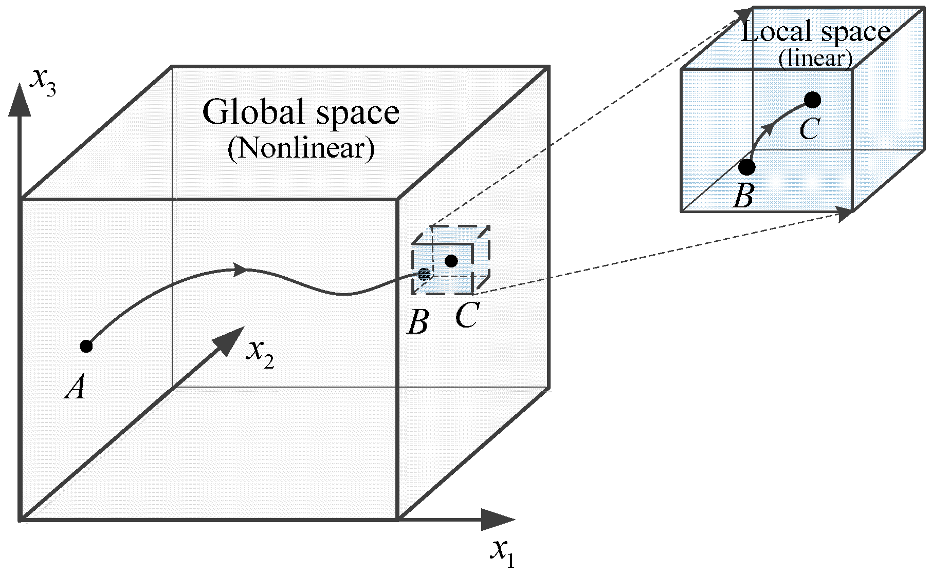
The multi-scale properties can be described geometrically with a 3-dimensional example as in Figure 2. Due to the highly nonlinear properties, traditional optimization cannot be applied for the direct finding of the global optimum point C from a random start point A. However, the non-math- based coarse method can be easily used for coarse searching on a global scale. Once the proper point B near the optimum is found, then the model can be linearized at the local scale around the point B. Through this quantitative searching, the optimum point C can be found.

3. Weighted PSO-LM Algorithm for Multi-Scale Parameter Identification

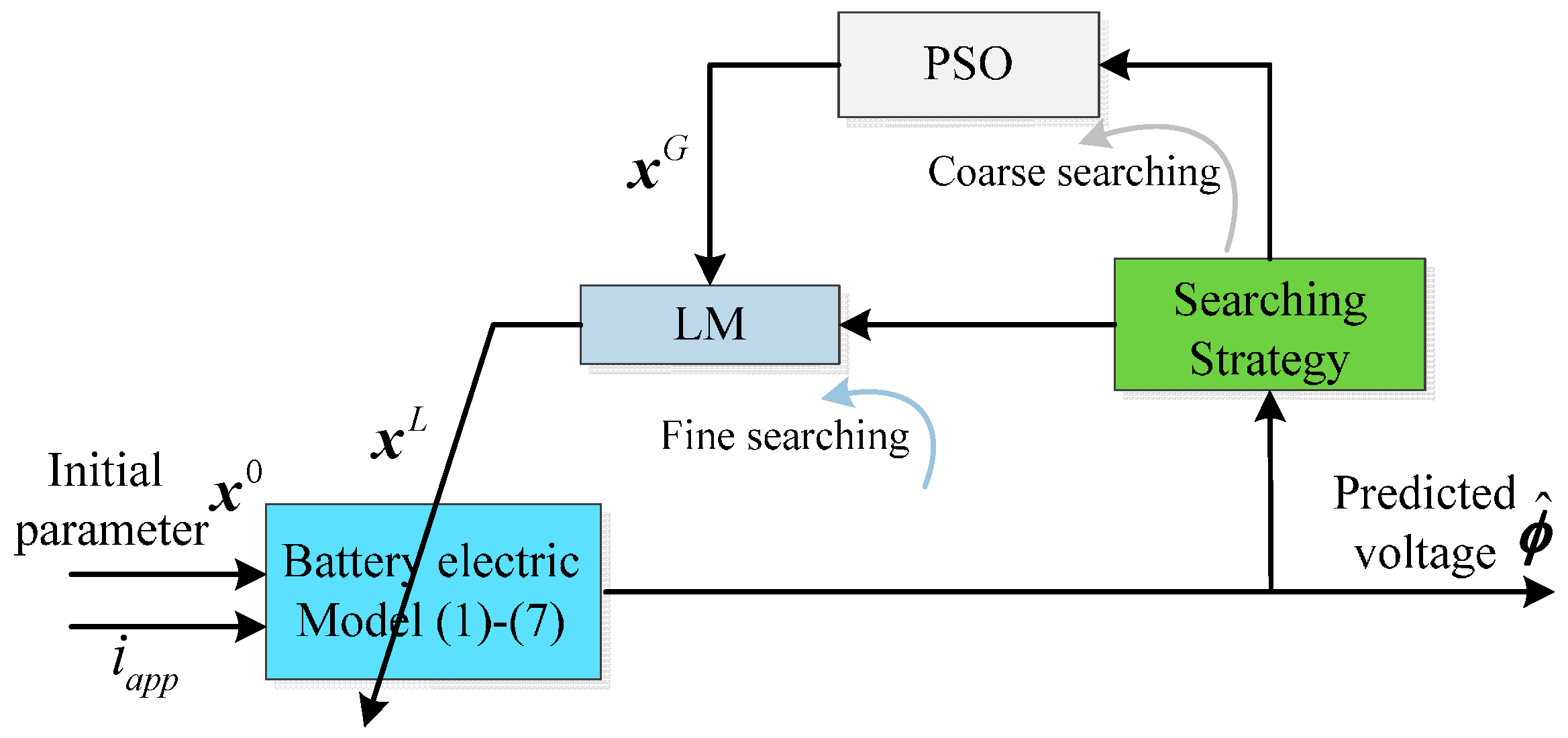
To address the problem of the multi-scale (global and local) complexity existing in the parameter identification, this section will provide a weighted PSO-LM combined algorithm for the multi-scale (coarse and fine) identification of parameter vector $\mathit{x}$. PSO is firstly utilized to implement the coarse-scale parameter identification to find the near-optimal point in the global space. Then the LM algorithm is embedded in PSO to conduct the fine-scale parameter identification in the vicinity of the optimum within the local space. The block diagram of the PSO-LM based identification approach is illustrated in Figure 3.

3.1. Search Strategy

The search strategy determines whether PSO or LM is suitable for the next step identification. An objective/fitness function $f$ is embedded in the search strategy as a criterion for the decision making. The strategy consists of two steps:

(1)

Coarse searching: The identification procedure is assured to start from PSO by initializing a group of random parameter vectors in the global parameter space. After several generations of PSO optimization, a near-global optimum is acquired;

(2)

Fine searching: The identification procedure is then switched to LM by starting from the near-global optimum with the gradient search in a local space. The identified parameter vector is compared with the one obtained in PSO to select a better candidate to enter the next iteration.

The objective/fitness function $f$ is constructed for the optimal identification of the parameter vector $\mathit{x}$ in the battery electric model (1)–(7), which is a quadratic function of the difference between the experimental terminal voltage ${\varphi }_k$ and the predicted voltage ${\widehat{\varphi }}_k$ with additional parameters $w_k>0$, $k\in \{1,2,\cdots ,N\}$:

$$f={\displaystyle \sum _{k=1}^{k=N}{w}_k{({\varphi }_k-{\widehat{\varphi }}_k)}^2}={(\mathit{\varphi }-\widehat{\mathit{\varphi }})}^T\mathit{W}(\mathit{\varphi }-\widehat{\mathit{\varphi }})$$

(8)

where $N$ is the number of fitting curves, $\mathit{\varphi }\triangleq {[{\varphi }_1,{\varphi }_2,\cdots ,{\varphi }_N]}^T$ and $\widehat{\mathit{\varphi }}$ is the estimation of $\mathit{\varphi }$, both are vectors consisting of ${\varphi }_k$ and ${\widehat{\varphi }}_k$, $k\in \{1,2,\cdots ,N\}$, respectively, $\mathit{W}\triangleq \mathrm{diag}\{w_1,w_2,\cdots ,w_N\}$ is the parametric matrix assigned to obtain a better fitness.

In what follows, we will define the specified form of the parameter matrix $\mathit{W}$, whose element $w_k$ is applied to the $k$-th experimental terminal voltage curve:

$$w_k={\gamma }_k{\chi }_k$$

(9)

where ${\gamma }_k$ takes into account the experimental deviations in the k-th voltage curve and is defined as:

$${\gamma }_k=\frac{1}{\frac{{\sigma }_k^2}{{\displaystyle \sum _{k=1}^N{N}_k}}\left[{\displaystyle \sum _{k=1}^N{\displaystyle \sum _{j=1}^{N_k}\frac{1}{{\sigma }_j^2}}}\right]}$$

(10)

with ${\sigma }_k\triangleq \sqrt{\frac{1}{N_k-1}{\displaystyle \sum _{j=1}^{N_k}{({\widehat{\varphi }}_{k,j}-{\varphi }_{k,j})}^2}}$, in which ${\widehat{\varphi }}_{k,j}$ is the predicted voltage of the j-th point in the k-th curve and obtained by calculating the difference between ${\widehat{\varphi }}_{k,j}^p$ and ${\widehat{\varphi }}_{k,j}^n$, ${\varphi }_{k,j}$ is the experimental voltage at the j-th point in the k-th curve, $N_k$ is the number of experimental data points in the k-th voltage curve. The parameter ${\chi }_k$ is proportional to the difference between the previous voltage predictions and the experimental data in the k-th voltage curve and is defined as:

$${\chi }_k=1+\frac{(w_{k,\max }-1){\eta }_k}{{\eta }_{k,\max }}$$

(11)

where $w_{k,\max }>1$ is a given constant, ${\eta }_k\triangleq \left|{\widehat{\varphi }}_k-{\varphi }_k\right|$, ${\eta }_{k,\max }$ is the maximum value of ${\eta }_k$ for each $k\in \{1,2,\cdots ,N\}$. Obviously, the parameter ${\chi }_k$ varies between 1 and $w_{k,\max }$, that is, ${\chi }_k=1$ for the best fitting points and ${\chi }_k=w_{k,\max }$ for the worst fitting ones.

3.2. Implementation of PSO-LM Algorithm

The PSO algorithm adopted here is a variation of conventional PSO, named hybrid multi-swarm PSO (HMPSO). The HMPSO method divides the swarm into several sub-swarms, and adopts a parallel PSO search operator for the sub-swarms [30]. For a particle swarm with a population consisting of M $\overline{n}$-dimensional particles, the velocity $v_{i,j}^m$ and position $x_{i,j}^m$, $i\in \{1,2,\cdots ,M\}$, $j\in \{1,2,\cdots ,\overline{n}\}$ of the j-th dimension of the i-th particle are updated as [30]:

$$\{\begin{array}{l}{\mathit{v}}_{i,j}^{m+1}=\left|{\gamma }_1\right|({\mathit{\xi }}_{i,j}^m-{\mathit{x}}_{i,j}^m)+\left|{\gamma }_2\right|({\mathit{\psi }}_{i,j}^m-{\mathit{x}}_{i,j}^m)\\ x_{i,j}^{m+1}=x_{i,j}^m+v_{i,j}^{m+1}\end{array}$$

(12)

where ${\mathit{\xi }}_{i,j}^m$ and ${\mathit{\psi }}_{i,j}^m$ are the best previous position of $x_{i,j}^m$ and the best position achieved with its neighbors at the m-th generation, respectively; ${\gamma }_1$ and ${\gamma }_2$ are two separately generated random numbers with uniform distribution in the range of $[0,1]$. The privilege of HMPSO lies in that it can explore more promising regions of the search space by applying differential evolution (DE) to update the personal best of each particle. In conclusion, it is a more competitive and effective PSO method for solving optimizing problems. For more details on the HMPSO algorithm, please refer to ref. [30].

The LM algorithm has a strong ability to find a local and more optimistic result. The parameter correction vector $\mathrm{\Delta }\mathit{x}$ is obtained based on the objective Function (8) and the Marquardt method as follows:

$$\mathrm{\Delta }\mathit{x}={({\mathit{J}}^T\mathit{W}\mathit{J}+\lambda \mathit{I})}^{-1}{\mathit{J}}^T\mathit{W}(\mathit{\varphi }-\widehat{\mathit{\varphi }})$$

(13)

where $\mathit{J}$ is a matrix of partial derivatives of the terminal voltage with respect to the fitting parameter vector $\mathit{x}$ evaluated at all the experimental voltage data. LM adaptively alters the algorithmic parameter value $\lambda$ updates between the gradient descent method and the Gauss-Newton method. The parameter $\lambda$ determines how the LM algorithm works and is initialized to be large. If the iteration results in a better approximation, then the parameter $\lambda$ is decreased to $0.1\lambda$ and LM is more like a Gauss-Newton update one. If the iteration provides a worse approximation, then the parameter $\lambda$ is increased to $10\lambda$ and LM approaches that of the gradient descent update. The details of LM can refer to [17].

The proposed PSO-LM algorithm is a hybrid multi-scale approach to determine the value of $\mathit{x}$ in the battery model (1)–(7) based on the fitness Function (8). It not only improves the convergence rate and effectively escapes from the stagnation of PSO, but also overcomes the drawback of the local minimum entrapment of LM. The pseudo code of the suggested weighted PSO-LM algorithm is shown in

Table 1. Implementation of PSO-LM algorithm.

Step 1	Initialize the PSO population size, dimensions, and termination conditions, i.e., randomly generate an initial swarm P0 consisting of M seven-dimensional particles, ${\mathit{x}}_i^0={[\begin{array}{cccc}{x}_{i,1}^0& x_{i,2}^0& \cdots & x_{i,7}^0\end{array}]}^T$, $i\in \{1,2,\cdots ,M\}$, optimization error ($f_{\mathrm{set}}$); Initialize the LM parameters, i.e., $\lambda$ and the maximum number of iteration $R_{\mathit{max}}$;
Step 2	Calculate the potential ${\widehat{\mathit{\varphi }}}_i$, parameter matrix $\mathit{W}$, and the fitness value $f({\mathit{x}}_i^0)$ given in (7) for each particle, $i\in \{1,2,\cdots ,M\}$;
Step 3	Record particle’s personal bests, i.e., ${\mathit{\xi }}_1^0,{\mathit{\xi }}_2^0,\cdots ,{\mathit{\xi }}_M^0$;
Step 4	while ($\mathrm{fitness}\mathrm{value}<f_{\mathrm{set}}$) do
Step 5	Update the personal best ${\mathit{\xi }}_i^m$ at m-th generation using the differential evolution (DE), and evaluate the fitness value $f({\mathit{\xi }}_i^m)$ for the personal best;
Step 6	Split the swarm Pm into several sub-swarms, and each sub-swarm evolves in parallel according to the governing equations of the particles’ velocity and position: ${\mathit{v}}_i^{m+1}=\left|{\gamma }_1\right|({\mathit{\xi }}_i^m-{\mathit{x}}_i^m)+\left|{\gamma }_2\right|({\mathit{\psi }}_i^m-{\mathit{x}}_i^m)$ ${\mathit{x}}_i^{m+1}={\mathit{x}}_i^m+{\mathit{v}}_i^{m+1}$ where ${\gamma }_1$ and ${\gamma }_2$ are two scalars generated randomly in the range of (0, 1), and ${\mathit{\psi }}_i^m$ is the best position achieved with its neighbors;
Step 7	Calculate the potential ${\widehat{\mathit{\varphi }}}_i$, parameter matrix $\mathit{W}$, and the fitness value $f({\mathit{x}}_i^{m+1})$ for each particle ${\mathit{x}}_i^{m+1}$, $i\in \{1,2,\cdots ,M\}$; Let ${\mathit{x}}_i^{\ast }\leftarrow {\mathit{x}}_i^{m+1}$ and $f_i^{\ast }\leftarrow f({\mathit{x}}_i^{m+1})$; Set ${\mathit{x}}_i^{\ast }$ be the initial values of LM algorithm;
Step 8	for $i=1:M$ do
Step 9	while ($\mathit{iter}<R_{\mathit{max}}$ and $f_i^{\ast }>f_{\mathrm{set}}$) do
Step 10	Calculate Jacobin matrix ${\mathit{J}}_i=[\partial {\widehat{\mathit{\varphi }}}_i/\partial x_0,\partial {\widehat{\mathit{\varphi }}}_i/\partial x_1,\dots ,\partial {\widehat{\mathit{\varphi }}}_i/\partial x_6]$, parameter matrix $\mathit{W}$, Hessian matrix ${\mathit{H}}_i={\mathit{J}}_i^T{\mathit{W}}_i{\mathit{J}}_i$; Calculate the potential ${\widehat{\mathit{\varphi }}}_i$ and $f_i^{\ast }$ at current particle ${\mathit{x}}_i^{\ast }$;
Step 11	Update the Hessian matrix ${\mathit{H}}_i={\mathit{H}}_i+\lambda \mathit{I}$, the parameter correction vector $\mathrm{\Delta }{\mathit{x}}_i={\mathit{H}}_i^{-1}{\mathit{J}}_i^T({\widehat{\mathit{\varphi }}}_i-{\mathit{\varphi }}_i)$, the particle position ${\mathit{x}}_i^{lm}={\mathit{x}}_i^{\ast }+\mathrm{\Delta }{\mathit{x}}_i$, and the potential ${\widehat{\mathit{\varphi }}}_i$, the fitness value $f_i^{lm}$ at the current particle ${\mathit{x}}_i^{lm}$;
Step 12	if $f_i^{lm}<f_i^{\ast }$ do
	$\lambda =\lambda /10$, ${\mathit{x}}_i^{\ast }\leftarrow {\mathit{x}}_i^{lm}$, $f_i^{\ast }\leftarrow f_i^{lm}$ and go back to Step 10;
	else
	$\lambda =\lambda \times 10$, go back to Step 11;
	end if
Step 13	$\mathrm{iter}=\mathrm{iter}+1$;
Step 14	end while
Step 15	$f({\mathit{x}}_i^{m+1})\leftarrow f_i^{\ast },{\mathit{x}}_i^{m+1}\leftarrow {\mathit{x}}_i^{\ast }$; $i=i+1$;
Step 16	end for
Step 17	$m=m+1$;
Step 18	end while
Step 19	Output the identified parameter vector $\mathit{x}$.

. The coarse-searching procedure of PSO can be found from Step 1 to Step 6, and the fine-searching procedure of LM is embedded from Step 7 to Step 16.

4. Experimental Validation

4.1. Experimental Setup

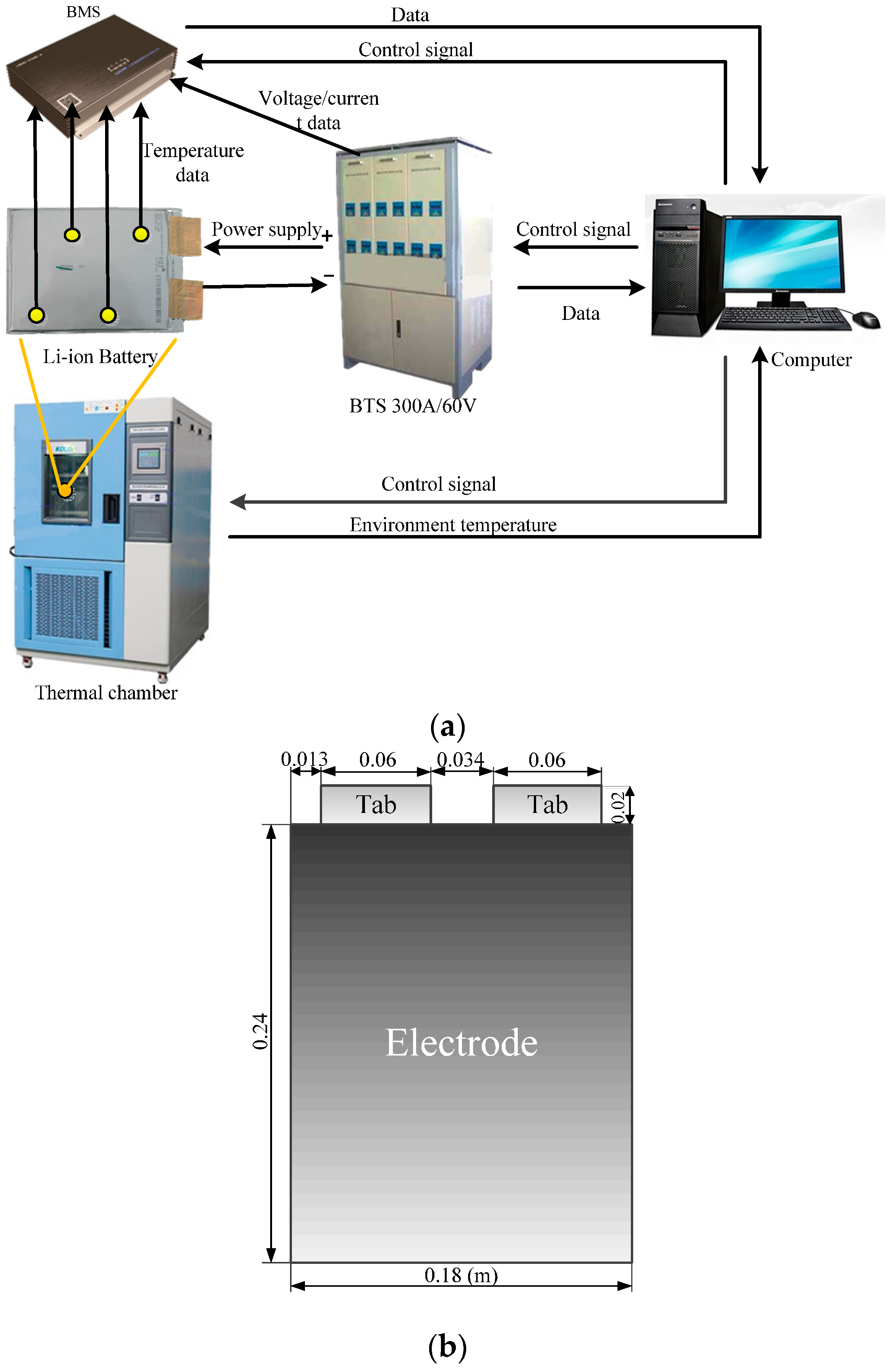
To illustrate the validity of the proposed PSO-LM algorithm, discharge experiments are carried out for a 60 Ah LIB (LiFePO₄) at a constant temperature of 25 °C on the experimental platform shown in Figure 4a. This platform consists of a thermal chamber, lithium-ion battery, battery testing system (BTS-300 A/60 V, Shenzhen Neware Technology, Shenzhen, China), battery management system (BMS) and computer. The schematic diagram of the signal and data flow for the experimental platform is also shown in Figure 4a. Figure 4b shows the dimensions of electrodes and positions of the tabs of a 60 Ah LIB. The discharge and charge tests of the battery are completed on this platform. The battery is first fully charged and then discharged at various discharging rates namely 1C (60 A), 2C (120 A) and 3C (180 A) until the cut-off voltage. The experimental terminal voltage data is collected per second during its discharge. Subsequently, the battery is fully discharged and then charged at various charging rates namely 1C, 2C and 3C until the cut-off voltage. The experimental terminal voltage data is also collected during the charging process. Due to the hysteresis behavior existed in battery, the voltage curves during discharge do not agree with that during charge process and thus are fitted separately [27]. There will be two sets of parameters $x_1-x_7$ and $x_1^{*}-x_7^{*}$ for these two processes, respectively.

4.2. Numerical Calculation and Parameter Setup

The numerical solutions of the battery electric model (1)–(7) subjected to the associated boundary conditions are obtained by COMSOL (COMSOL Inc., Stockholm, Sweden), which is a commercial software package for accurate numerical simulation of partial differential equations (PDEs) using the finite element method. The simulation results and identified parameters are exchanged through the interface of COMSOL with MATLAB (The MathWorks Inc., Natick, MA, USA). In the proposed PSO-LM algorithm, set $\lambda =0.1$, $R_{\mathit{max}}=20$, $M=16$, and for the parameter matrix $\mathit{W}$, set $N=3$, $w_{1,\max }=4,w_{2,\max }=8$ and $w_{3,\max }=10$.

4.3. Results and Discussion

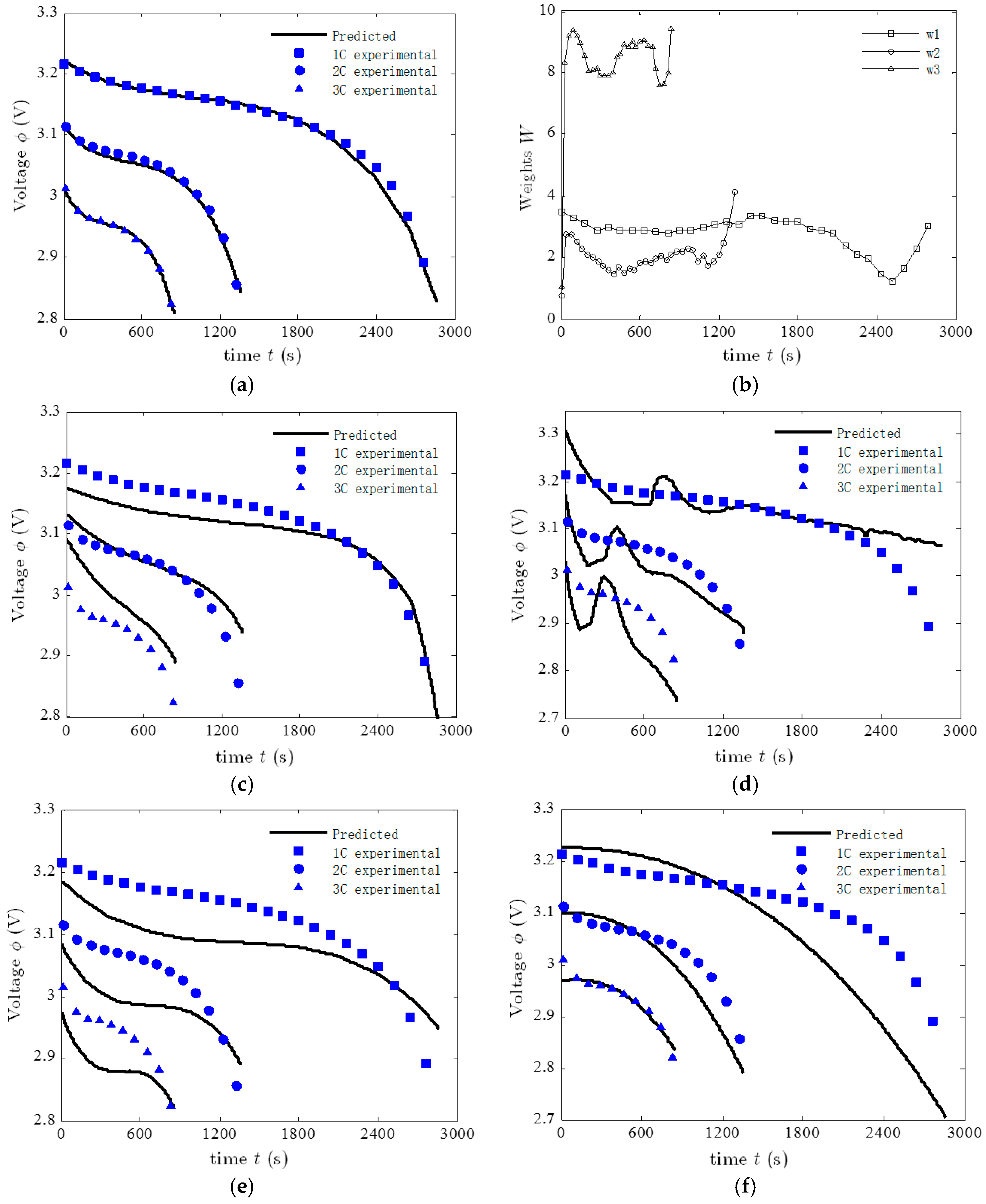
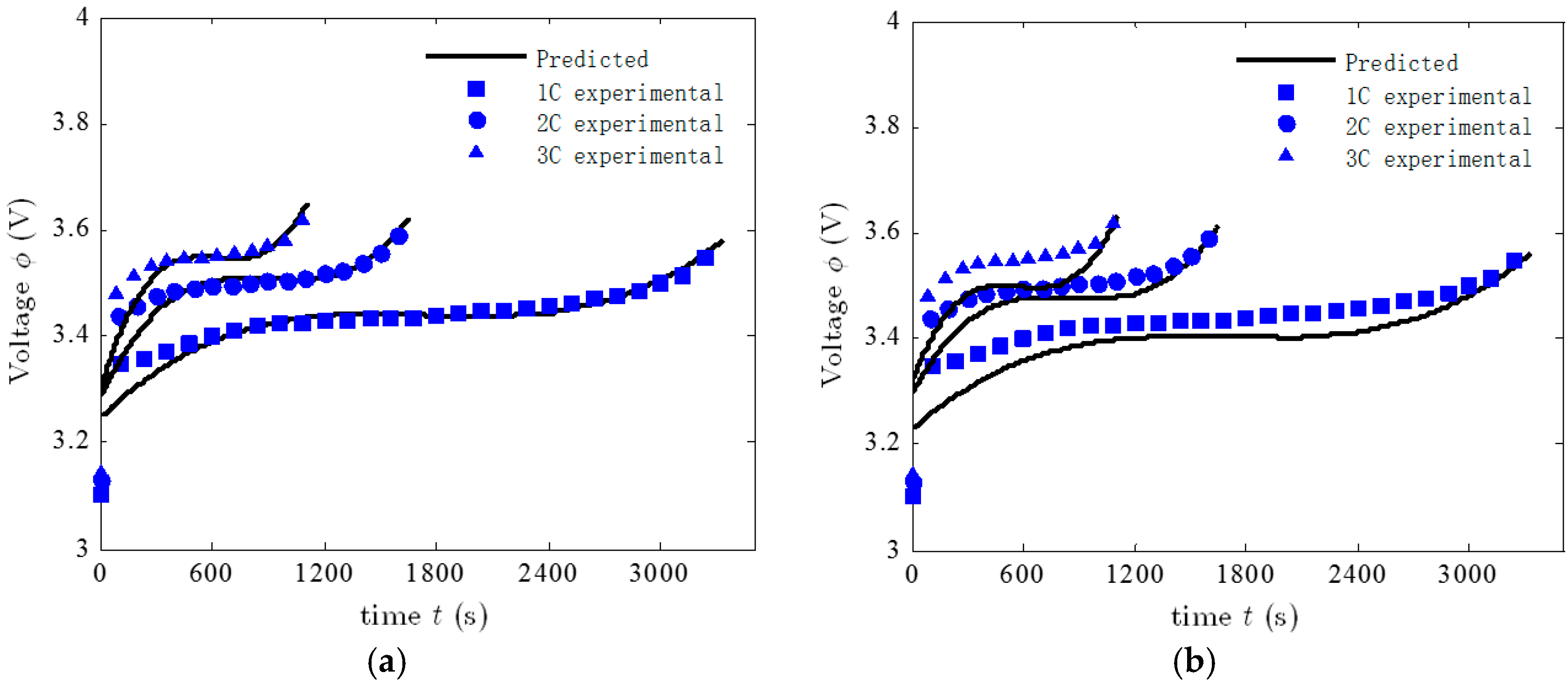
The value of the parameter vector x in the battery electric model (1)–(7) is identified using the proposed algorithm through fitting the three experimental terminal voltage curves simultaneously.

Table 2. The identified value of the parameter vector x during discharge.

Parameter	${\mathit{x}}_{\mathit{1}}$	${\mathit{x}}_{\mathit{2}}$	${\mathit{x}}_{\mathit{3}}$	${\mathit{x}}_{\mathit{4}}$	${\mathit{x}}_{\mathit{5}}$	${\mathit{x}}_{\mathit{6}}$	${\mathit{x}}_{\mathit{7}}$
Identified value	$3.125$	$-5.077\times {10}^{-1}$	$1.492$	$-1.768$	$1.286\times {10}^4$	$-6.177\times {10}^1$	$-2.377\times {10}^3$

gives the identified value of the parameter vector x. As shown in Figure 5a, the predictions with identified parameter vector x and measurements of the terminal voltage curves are well matched with each other, and this demonstrates the effectiveness of the proposed method. Figure 5b depicts the corresponding trajectory of the weight matrix $\mathit{W}=\mathrm{diag}\{w_1,w_2,w_3\}$.

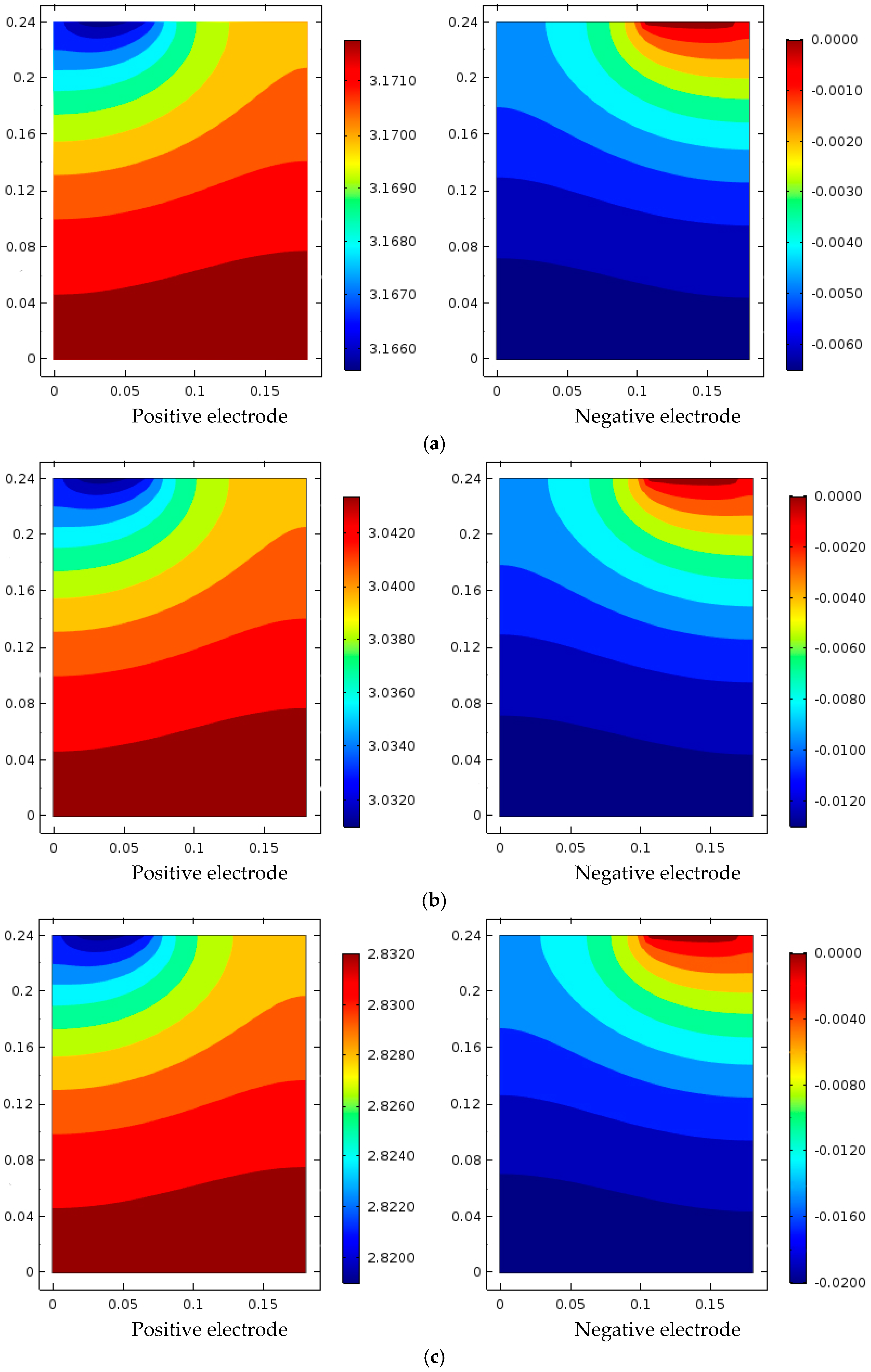
The potential distributions on the positive and negative electrodes during discharge are obtained as a function of time for various discharge rates of 1C, 2C, and 3C. For example, Figure 6 indicates the potential distributions on the positive and negative electrodes with discharge rates of 1C, 2C, and 3C at discharge time $t=14\min$, respectively. Because all the current flows into the tab from the entire electrode plate, the potential gradient on the positive electrode shown in Figure 6 is seen to be most severe in the region near to the tab. While the potential gradient on the negative electrode is also the highest in the region near tab. This is because all the current has to flow from the tab through the entire electrode plate.

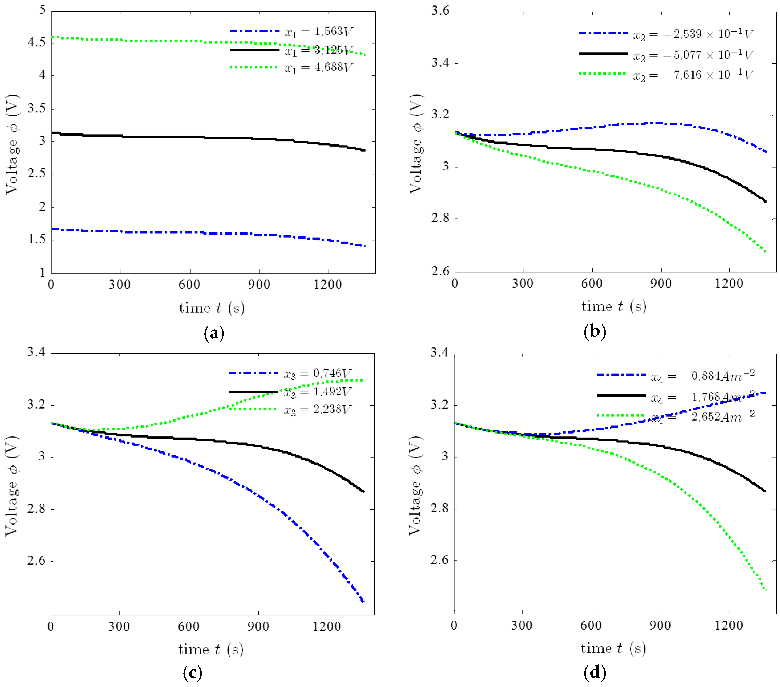
To demonstrate the advantage of the proposed weighted PSO-LM algorithm, a comparison study is also conducted among PSO, PSO-LM with $\mathit{W}=\mathrm{diag}\{1,1,1\}$, weighted PSO-LM, LM and the method of trial and error. Figure 5 also compares the experimental and predicted terminal voltage curves at discharge rates of 1C, 2C, and 3C through the simultaneous fit by PSO-LM with $\mathit{W}=\mathrm{diag}\{1,1,1\}$ (Figure 5c), PSO (Figure 5d), LM (Figure 5e) and method of trial and error adopted in [29] (Figure 5f). It is clear from Figure 5 that the proposed weighted PSO-LM algorithm provides a more accurate discharging curve fitness compared to the other algorithms. Moreover, although the fitting result of PSO-LM with $\mathit{W}=\mathrm{diag}\{1,1,1\}$ is better than that of PSO, it is worse than that of weighted PSO-LM. This is because the same weights are assigned to different curves but without considering the difference of the data number of each voltage curve (e.g., there are 2860 data points for the 1C-discharging voltage curve, 1360 data points for 2C and 850 for 3C). To evaluate the parameter importance, an a-priori sensitivity analysis is carried out for the identified parameters [27]. Each parameter is tuned to 0.5 times and 1.5 times the identified value. The results, shown in Figure 7, indicate that for the same range of parameter values, $x_6$ and $x_7$ are less sensitive than other parameters and hence can be held constant, while the other five parameters $x_1-x_5$ are very sensitive and deserve more attention during the identification.

A further quantized research needs to be carried to determine the importance order of parameters $x_1-x_5$. On the other hand, Figure 7 shows that $x_1$ and $x_5$ have the similar effect toward model output, while $x_2$, $x_5$ and $x_4$ have the similar effect.

4.3.1. 95% Confidence Interval

From a statistical point of view, it is very useful to obtain the confidence interval instead of the point estimation for the fitting parameter vector x [31]. In this paper, the 95% confidence interval of the parameter vector x is calculated as follows:

$$x_i^{\ast }-{\mathcal{T}}_{(1-0.05/2)}{S}_E\sqrt{a_{ii}}\le x_i\le x_i^{\ast }+{\mathcal{T}}_{(1-0.05/2)}{S}_E\sqrt{a_{ii}}$$

(14)

where $x_i^{\ast }$ is the point estimation of the parameter $x_i$, $i\in \{1,2,\cdots ,7\}$, ${\mathcal{T}}_{(1-0.05/2)}$ is a value of $\mathcal{T}$-distribution with ($\overline{N}-7$) degrees of freedom, $S_E$ is the unbiased estimate of unknown variance $\sigma$ and is calculated by $S_E=\sqrt{\frac{1}{\overline{N}-7}{\displaystyle \sum _{\varsigma =1}^N{\displaystyle \sum _{j=1}^{N_{\varsigma }}{({\varphi }_{\varsigma ,j}-{\widehat{\varphi }}_{\varsigma ,j})}^2}}}$, $\overline{N}$ is the number of experimental data points and derived by $\overline{N}={\displaystyle \sum _{\varsigma =1}^N{N}_{\varsigma }}$, and $a_{ii}$ is the i-th main diagonal element of ${({\mathit{J}}^T\mathit{J})}^{-1}$.

To demonstrate the goodness of the simultaneous fit, the model (1)–(7) is also to fit each experimental curve independently for comparison. The 95% confidence intervals of all seven parameters obtained from both the simultaneous fit and three independent fits are presented in

Table 3. Comparison of the 95% confidence intervals of x estimated from the simultaneous fit and the independent fit.

Parameter	Simultaneous Fit	Independent Fit (1C)	Independent Fit (2C)	Independent Fit (3C)
$x_1$	$3.125\pm 0.0012$	$3.094\pm 0.02895$	$2.844\pm 0.1022$	$2.619\pm 6.178$
$x_2$	$(-5.077\pm 0.1509)\times {10}^{-1}$	$(-2.929\pm 1.834)\times {10}^{-1}$	$(-3.305\pm 4.461)\times {10}^{-1}$	$-0.3632\pm 2.268$
$x_3$	$(1.492\pm 0.4326)\times {10}^{-1}$	$1.092\pm 0.4250$	$1.373\pm 0.05091$	$1.444\pm 1.481$
$x_4$	$(-1.768\pm 0.3626)\times {10}^{-1}$	$-1.465\pm 0.2131$	$-1.748\pm 0.04607$	$-1.723\pm 0.4383$
$x_5$	$12860\pm 13.14$	$(1.184\pm 0.3005)\times {10}^4$	$(1.017\pm 0.3847)\times {10}^4$	$(1.043\pm 16.28)\times {10}^4$
$x_6$	$(-0.6177\pm 4.021)\times {10}^2$	$(6.047\pm 21.10)\times {10}^3$	$(4.049\pm 2.459)\times {10}^3$	$(4.429\pm 77.02)\times {10}^3$
$x_7$	$(-2.377\pm 0.7177)\times {10}^3$	$(2.298\pm 24.41)\times {10}^3$	$(-5.160\pm 3.377)\times {10}^2$	$(-2.390\pm 55.73)\times {10}^3$
$S_E$	0.0079	0.0019	0.0037	0.0041

. Although Table 3 shows that each independent fit leads to a smaller $S_E$ compared to the simultaneous fit, the value of $S_E$ for the simultaneous fit is also acceptable.

4.3.2. 95% Joint Confidence Region

We know from [17] that the individual confidence interval cannot reflect the correlations between the parameters in the nonlinear system. Hence it is necessary to construct the joint confidence region. The 95% joint confidence regions of the parameter vector $\mathit{x}$ are calculated by Equation (15) [17]:

$$\frac{{(\mathit{x}-\widehat{\mathit{x}})}^T({\mathit{J}}^T\mathit{J})(\mathit{x}-\widehat{\mathit{x}})}{7{S_E}^2}\le F_{1-\alpha }(7,\overline{N}-7)$$

(15)

where $\mathit{x}$ is any point in the confidence region, $\widehat{\mathit{x}}$ is the point estimation value, $F_{1-\alpha }(7,\overline{N}-7)$ is the quantile function of the F-distribution with $7$ and $\overline{N}-7$ degree of freedom, $\alpha$ is the statistical significance level. Set $\alpha =0.05$, we get from the F-distribution table that $F_{0.95}(7,\overline{N}-7)=2.0986$. Without loss of generality, set $\widehat{\mathit{x}}$ to be the estimate of $x$ from weighted PSO-LM, i.e., $\widehat{\mathit{x}}={\mathit{x}}^{\ast }$, we have:

$$\mathit{x}-\widehat{\mathit{x}}=\mathit{x}-{\mathit{x}}^{\ast }=\left[\begin{array}{c}{x}_1-3.125\\ x_2+5.077\times {10}^{-1}\\ x_3-1.492\\ x_4+1.768\\ x_5-1.286\times {10}^4\\ x_6+6.177\times {10}^1\\ x_7+2.377\times {10}^3\end{array}\right]$$

(16)

The confidence regions are obtained from the following equation:

$${(x_i-x_i^{\ast })}^2{({\mathit{J}}^T\mathit{J})}_{ii}\le F_{0.95}(7,\overline{N}-7)7{S_E}^2$$

(17)

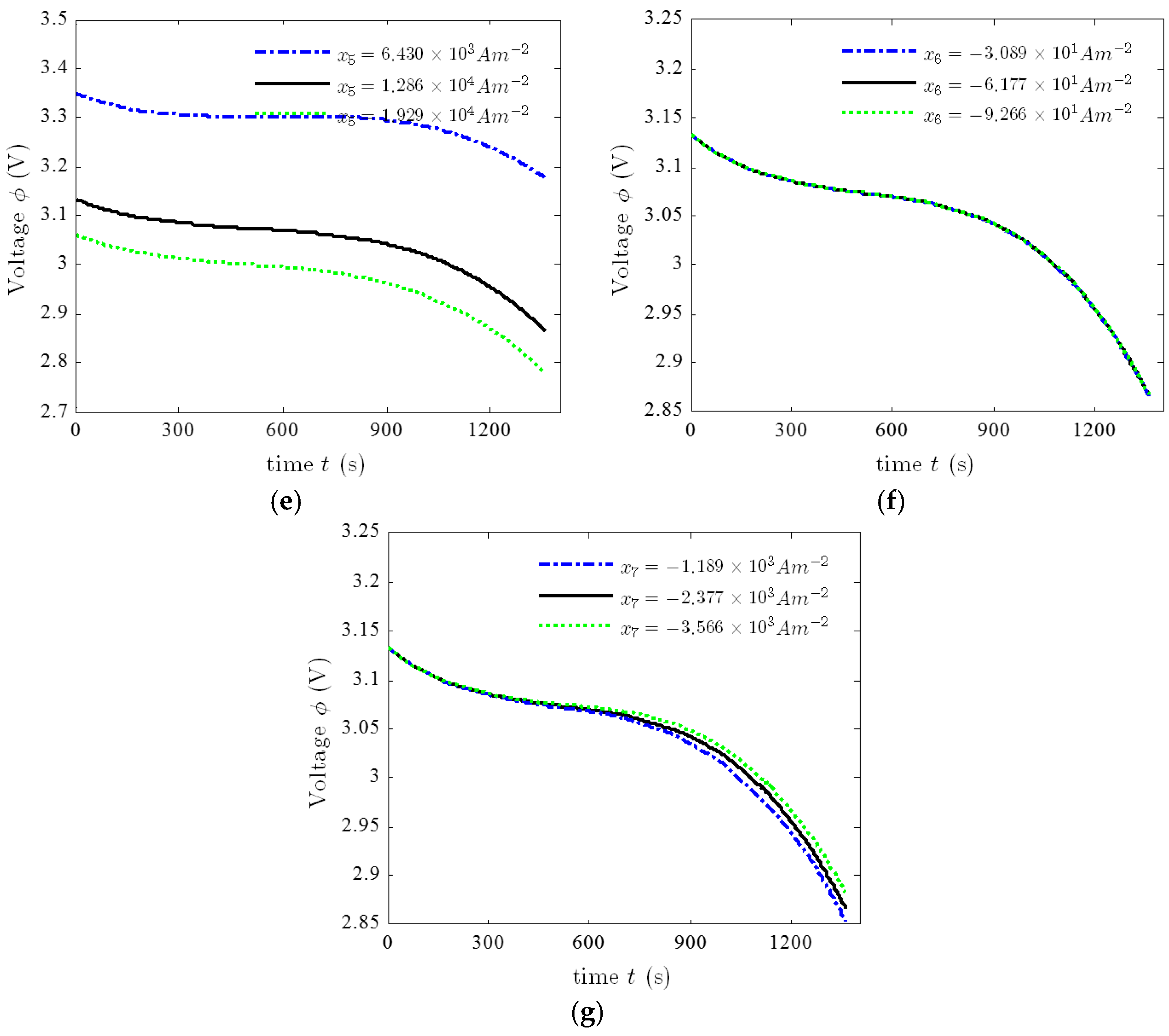
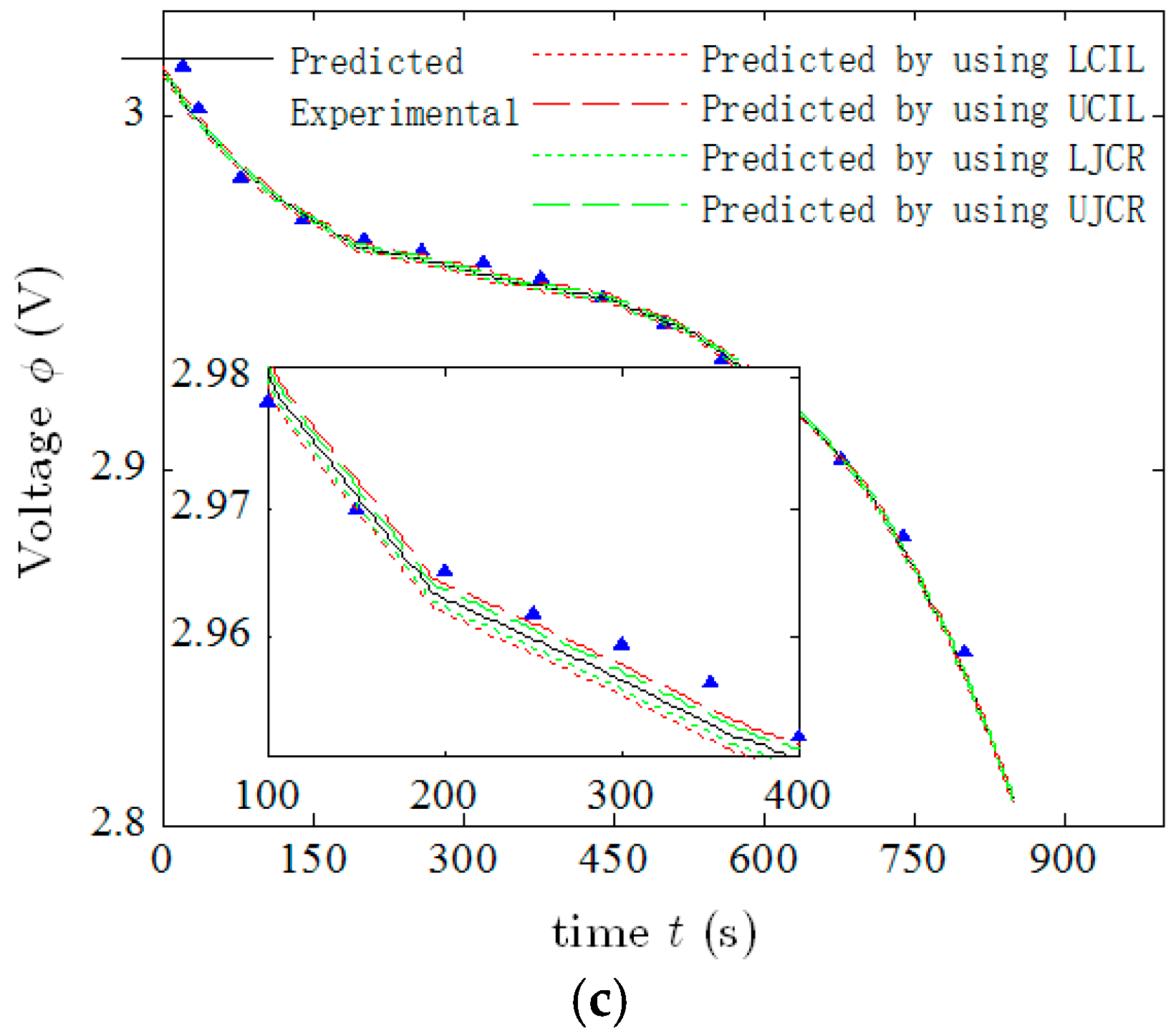
The confidence region of $x_1$ is obtained from Equation (16) by fixing the parameters $x_2,x_3,\cdots ,x_7$ to their estimation value. The 95% joint confidence regions of all seven parameters obtained from the simultaneous fit are given in

Table 4. The 95% joint confidence regions (CR) obtained from the simultaneous fit.

Parameter	${\mathit{x}}_{\mathit{1}}$	${\mathit{x}}_{\mathit{2}}$	${\mathit{x}}_{\mathit{3}}$	${\mathit{x}}_{\mathit{4}}$
CR	$3.125\pm 6.762\times {10}^{-4}$	$-(5.077\pm 0.015)\times {10}^{-1}$	$1.492\pm 2.355\times {10}^{-3}$	$-1.768\pm 3.442\times {10}^{-3}$
Parameter	${\mathit{x}}_{\mathit{5}}$	${\mathit{x}}_{\mathit{6}}$	${\mathit{x}}_{\mathit{7}}$
CR	$1.286\times {10}^4\pm 13.83$	$(-6.177\pm 6.78)\times {10}^1$	$(-2.377\pm 0.1052)\times {10}^3$

. The comparison of 95% joint confidence regions and 95% conference intervals of three simulated voltage curves is plotted in Figure 8. It can be observed from Table 4 and Figure 8 that the values of the parameter vector $\mathit{x}$ defined by the confidence region lead to less uncertainty in model predictions than those defined by the confidence interval.

As shown in Table 3 and Table 4, the confidence interval and confidence region of parameter $x_6$ are much larger than any of other six parameters. This phenomenon is caused by the parameter correlations as explained by Evans and White [32]. Thus, a thorough correlation analysis of these seven parameters is conducted in what follows.

4.3.3. Correlation Analysis

The correlation coefficient matrix $\mathit{R}$ of the parameters $x_i$, $i\in \{1,2,\cdots ,7\}$ is a symmetric matrix. Its elements $r_{ij}$ have all their values in the range $-1\le r_{ij}\le 1$, are calculated as follows:

$$r_{ij}=\frac{a_{ij}}{\sqrt{a_{ii}{a}_{jj}}},i,j\in \{1,2,\cdots ,7\},$$

(18)

Let matrix $\mathit{H}={\mathit{J}}^T\mathit{J}$, then $a_{ij}$, $i,j\in \{1,2,\cdots ,7\}$ are the elements of ${\mathit{H}}^{-1}$ after the simultaneous fit, and $a_{ii}$ is the i-th main diagonal element of ${\mathit{H}}^{-1}$. The matrix $\mathit{H}$ is calculated as:

$$\begin{array}{l}\mathit{H}={\mathit{J}}^T\mathit{J}=[\begin{array}{ccc}2.485\times {10}^3& 9.715\times {10}^2& 5.069\times {10}^2\\ 9.715\times {10}^2& 5.322\times {10}^2& 3.193\times {10}^2\\ 5.069\times {10}^2& 3.193\times {10}^2& 2.049\times {10}^2\\ 2.988\times {10}^2& 2.056\times {10}^2& 1.379\times {10}^2\\ -5.855\times {10}^{-2}& -3.445\times {10}^{-2}& -2.294\times {10}^{-2}\\ -1.896\times {10}^{-2}& -1.080\times {10}^{-2}& -6.631\times {10}^{-3}\\ -1.026\times {10}^{-2}& -6.685\times {10}^{-3}& -4.372\times {10}^{-3}\end{array}\\ \begin{array}{cccc}2.988\times {10}^2& -5.855\times {10}^{-2}& -1.896\times {10}^{-2}& -1.026\times {10}^{-2}\\ 2.056\times {10}^2& -3.445\times {10}^{-2}& -1.080\times {10}^{-2}& -6.685\times {10}^{-3}\\ 1.379\times {10}^2& -2.294\times {10}^{-2}& -6.631\times {10}^{-3}& -4.372\times {10}^{-3}\\ 9.592\times {10}^1& -1.664\times {10}^{-2}& -4.346\times {10}^{-3}& -2.990\times {10}^{-3}\\ -1.664\times {10}^{-2}& 5.942\times {10}^{-6}& 8.343\times {10}^{-7}& 5.756\times {10}^{-7}\\ -4.346\times {10}^{-3}& 8.343\times {10}^{-7}& 2.471\times {10}^{-7}& 1.545\times {10}^{-7}\\ -2.990\times {10}^{-3}& 5.756\times {10}^{-7}& 1.545\times {10}^{-7}& 1.027\times {10}^{-7}\end{array}].\end{array}$$

(19)

Hence, the matrix $\mathit{R}$ is obtained according to Equation (18):

$$\mathit{R}=\left[\begin{array}{ccccccc}1& -0.7211& 0.6311& -0.5489& -0.1471& 0.0731& -0.0592\\ -0.7211& 1& -0.9352& 0.7559& 0.5082& 0.3639& -0.3952\\ 0.6311& -0.9352& 1& -0.9278& -0.6087& -0.1230& 0.1899\\ -0.5489& 0.7559& -0.9278& 1& 0.5769& -0.2034& 0.1479\\ -0.1471& 0.5082& -0.6087& 0.5769& 1& 0.1564& -0.2760\\ 0.0731& -0.3639& -0.1230& -0.2034& 0.1564& 1& -0.9640\\ -0.0592& -0.3952& 0.1889& 0.1479& -0.2760& -0.9640& 1\end{array}\right]$$

(20)

The element $r_{ij}$ stands for the correlation between the $i$-th parameter and the $j$-th parameter, where $i$ stands for $x_i$, $i\in \{1,2,\cdots ,7\}$. As pointed out in [17], the absolute value of the elements of $\mathit{R}$ is closer to 1, the correlation between two parameters is higher. It is observed from the matrix $\mathit{R}$ given in Equation (20) that the values of all the main diagonal elements of $\mathit{R}$ are equal to 1. This indicates that each parameter is highly correlated with itself. We also observe from Equation (20) that the highest correlation between two different parameters occurs to the $x_6-x_7$ pair. A positive correlation coefficient between two parameters indicates that the errors causing the estimate of one parameter to be high also cause the other to be high, and vice versa. It is not difficult to conclude from $r_{67}=-0.9640$ that an underestimation of $x_6$ will cause an overestimation of $x_7$. Moreover, the eigenvectors and eigenvalues of $\mathit{R}$ can be applied to construct a hyperellipsoidal confidence region of the parameter space in the vicinity of the solution, where the model can be approximated linearized [17]. On the other hand, the high correlation between parameters also implies that it is difficult to obtain separate estimates of these parameters with the available data. The regression must be repeated and restarted from different initial parameter values many times to bypass the local minimum. While the multi-scale (global and local) approach provides a possible solution to find the global optima in this study.

4.4. Fitting to Charge Curves

The weighted PSO-LM algorithm is also applied to identify the parameters of $x_1^{*}-x_7^{*}$ during the charge process. The identified parameter values are in

Table 5. The identified value of the parameter vector ${\mathit{x}}^{*}$ during charge.

Parameter	${\mathit{x}}_{\mathit{1}}^{\mathit{*}}$	${\mathit{x}}_{\mathit{2}}^{\mathit{*}}$	${\mathit{x}}_{\mathit{3}}^{\mathit{*}}$	${\mathit{x}}_{\mathit{4}}^{\mathit{*}}$	${\mathit{x}}_{\mathit{5}}^{\mathit{*}}$	${\mathit{x}}_{\mathit{6}}^{\mathit{*}}$	${\mathit{x}}_{\mathit{7}}^{\mathit{*}}$
Identified value	3.370	−1.033	2.142	1.459	$1.078\times {10}^4$	$-3.101\times {10}^3$	$2.617\times {10}^3$

.

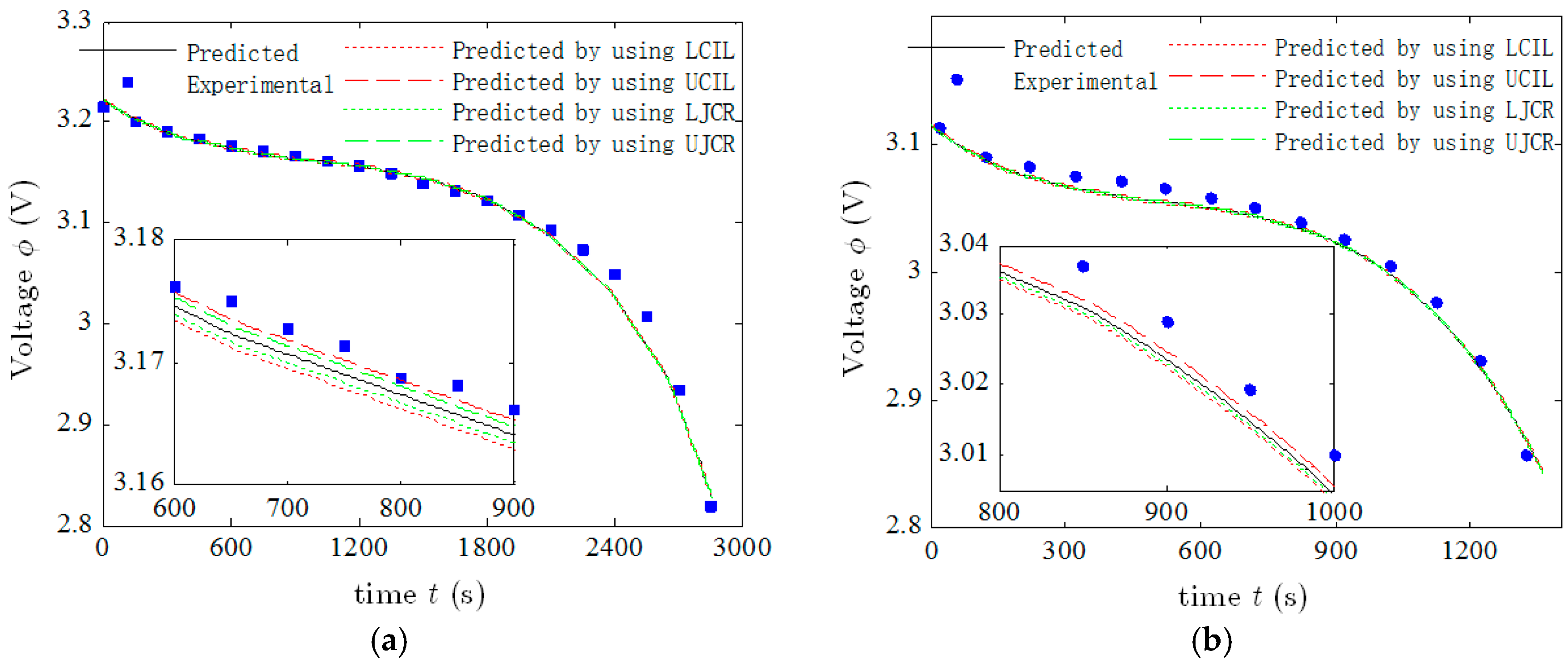
Figure 9 compares the experimental and predicted terminal voltages curves at charge rates of 1C, 2C, and 3C by the proposed PSO-LM algorithm and the method of trial and error adopted in [22]. It is concluded that the proposed PSO-LM algorithm provides a more accurate prediction than the method of trial and error. This result further demonstrates the effectiveness of the proposed multi-scale method. The analysis of the charge parameter values can refer to those during the discharge process, and thus is omitted.

5. Conclusions

A multi-scale parameter identification approach has been developed to identify the proper parameter value of the PDD model for the LIB during charge and discharge. This multi-scale approach is a combination of the PSO algorithm and the LM algorithm. PSO has the advantage of the coarse searching in large scale and LM has the advantage of the fine searching in small scale. Integration of them can effectively solve the difficult identification of the model with multi-scale complexity. To obtain a better fitness, a weighted objective/fitness function is implemented in this algorithm to reduce the difference among the multiple curves. The experimental results demonstrate the effectiveness of the proposed multi-scale identification approach.

References

- Scrosati, B.; Garche, J. Lithium batteries: Status, prospects and future. J. Power Sources 2010, 195, 2419–2430. [Google Scholar] [CrossRef]
- Lu, L.; Han, X.; Li, J.; Hua, J.; Ouyang, M. A review on the key issues for lithium-ion battery management in electric vehicles. J. Power Sources 2013, 226, 272–288. [Google Scholar] [CrossRef]
- Ramadesigan, V.; Northrop, P.W.C.; De, S.; Santhanagopalan, S.; Braatz, R.D.; Subramanian, V.R. Modeling and simulation of lithium-ion batteries from a systems engineering perspective. J. Electrochem. Soc. 2012, 159, R31–R45. [Google Scholar] [CrossRef]
- Santhanagopalan, S.; Zhang, Q.; Kumaresan, K.; White, R.E. Parameter estimation and life modeling of lithium-ion cells. J. Electrochem. Soc. 2008, 155, A345–A353. [Google Scholar] [CrossRef]
- Luo, W.; Lyu, C.; Wang, L.; Zhang, L. A new extension of physics-based single particle model for higher charge-discharge rates. J. Power Sources 2013, 241, 295–310. [Google Scholar] [CrossRef]
- Doyle, M.; Fuller, T.F.; Newman, J. Modeling of galvanostatic charge and discharge of the lithium polymer Insertion cell. J. Electrochem. Soc. 1993, 140, 1526–1533. [Google Scholar] [CrossRef]
- Kwon, K.H.; Shin, C.B.; Kang, T.H.; Kim, C.-S. A two-dimensional modeling of a lithium-polymer battery. J. Power Sources 2006, 163, 151–157. [Google Scholar] [CrossRef]
- Liu, Z.; Li, H. A Spatiotemporal estimation method for temperature distribution in lithium-ion batteries. IEEE Trans. Ind. Inform. 2014, 10, 2300–2307. [Google Scholar] [CrossRef]
- Wang, M.; Li, H.-X. Spatiotemporal modeling of internal states distribution for lithium-ion battery. J. Power Sources 2016, 301, 261–270. [Google Scholar] [CrossRef]
- Xiao, T.; Li, H.-X. Eigenspectrum-based iterative learning control for a class of distributed parameter system. IEEE Trans. Autom. Control 2017, 62, 824–836. [Google Scholar] [CrossRef]
- Xiao, T.; Li, H.-X. Sliding mode control design for a rapid thermal processing system. Chem. Eng. Sci. 2016, 143, 76–85. [Google Scholar] [CrossRef]
- Forman, J.C.; Moura, S.J.; Stein, J.L.; Fathy, H.K. Genetic identification and fisher identifiability analysis of the Doyle-Fuller-Newman model from experimental cycling of a LiFePO4 cell. J. Power Sources 2012, 210, 263–275. [Google Scholar] [CrossRef]
- Rahman, M.A.; Anwar, S.; Izadian, A. Electrochemical model parameter identification of a lithium-ion battery using particle swarm optimization method. J. Power Sources 2016, 307, 86–97. [Google Scholar] [CrossRef]
- Luzi, M.; Paschero, M.; Rizzi, A.; Massimo, F.; Mascioli, F. A PSO algorithm for transient dynamic modeling of lithium cells through a nonlinear RC filter. In Proceedings of the 2016 IEEE Congress on Evolutionary Computation, Vancouver, BC, Canada, 24–29 July 2016; pp. 279–286. [Google Scholar]
- Paschero, M.; Storti, G.L.; Rizzi, A.; Mascioli, F.M.F.; Rizzoni, G. A novel mechanical analogy-based battery model for SoC estimation using a multicell EKF. IEEE Trans. Sustain. Energy 2016, 7, 1695–1702. [Google Scholar] [CrossRef]
- Wang, M.; Li, H.-X. Real-time estimation of temperature distribution for cylindrical lithium-ion batteries under boundary cooling. IEEE Trans. Ind. Electron. 2017, 64, 2316–2324. [Google Scholar] [CrossRef]
- Constantinides, N.M.A. Numerical Methods for Chemical Engineers with MATLAB Applications; Prentice Hall PTR: Upper Saddle River, NJ, USA, 1999; pp. 440–485. [Google Scholar]
- Shen, W.; Li, H.-X. Parameter identification for the electrochemical model of li-ion battery. In Proceedings of the International Conference on System Science and Engineering (ICSSE), Nan Tou County, Taiwan, 7–9 July 2016; pp. 1–4. [Google Scholar]
- Hu, P.; Cao, G.; Zhu, X.; Li, J. Modeling of a proton exchange membrane fuel cell based on the hybrid particle swarm optimization with Levenberg-Marquardt neural network. Simul. Model. Pract. Theory 2010, 18, 574–588. [Google Scholar] [CrossRef]
- Nawi, N.M.; Rehman, M.; Aziz, M.A.; Herawan, T.; Abawajy, J.H. An accelerated particle swarm optimization based Levenberg Marquardt back propagation algorithm. In Proceedings of the International Conference on Neural Information Processing, Kuching, Malaysia, 3–6 November 2014; pp. 245–253. [Google Scholar]
- Cai, Z.; Wang, Y. A hybrid multi-swarm particle swarm optimization to solve constrained optimization problems. Front. Comput. Sci. 2009, 3, 38–52. [Google Scholar]
- Kim, U.S.; Yi, J.; Shin, C.B.; Han, T.; Park, S. Modelling the thermal behaviour of a lithium-ion battery during charge. J. Power Sources 2011, 196, 5115–5121. [Google Scholar] [CrossRef]
- Newman, J.; Tiedemann, W. Potential and current distribution in electrochemical-cells. J. Electrochem. Soc. 1993, 140, 1961–1968. [Google Scholar] [CrossRef]
- Tiedemann, W.; Newman, J. Current and potential distribution in lead-acid battery plates. J. Electrochem. Soc. 1979, 39–49. [Google Scholar]
- Gu, H. Mathematical analysis of a Zn/NiOOH cell. J. Electrochem. Soc. 1983, 130, 1459–1464. [Google Scholar] [CrossRef]
- Kim, U.S.; Yi, J.; Shin, C.B.; Han, T.; Park, S. Modeling the thermal behaviors of a lithium-ion battery during constant-power discharge and charge operations. J. Electrochem. Soc. 2013, 160, A990–A995. [Google Scholar] [CrossRef]
- Santhanagopalan, S. Parameter Estimation for Lithium Ion Batteries. Ph.D. Thesis, University of South Carolina, Columbia, SC, USA, January 2006. [Google Scholar]
- Kim, U.S.; Yi, J.; Shin, C.B.; Han, T.; Park, S. Modeling the dependence of the discharge behavior of a lithium-ion battery on the environmental temperature. J. Electrochem. Soc. 2011, 158, A611. [Google Scholar]
- Yi, J.; Kim, U.S.; Shin, C.B.; Han, T.; Park, S. Modeling the temperature dependence of the discharge behavior of a lithium-ion battery in low environmental temperature. J. Power Sources 2013, 244, 143–148. [Google Scholar] [CrossRef]
- Liu, H.; Cai, Z.; Wang, Y. Hybridizing particle swarm optimization with differential evolution for constrained numerical and engineering optimization. Appl. Soft Comput. 2010, 10, 629–640. [Google Scholar] [CrossRef]
- Fan, B.; Lu, X.; Li, H.-X. Probabilistic inference-based least squares support vector machine for modeling under noisy environment. IEEE Trans. Syst. Man Cybern. Syst. 2016, 46, 1703–1710. [Google Scholar] [CrossRef]
- Evans, T.I.; White, R.E. Estimation of electrode kinetic-parameters of the lithium/thionyl chloride cell using a mathematical-model. J. Electrochem. Soc. 1989, 136, 2798–2805. [Google Scholar] [CrossRef]
Figure 1.
Schematic diagram of the current flow in the parallel plate electrodes. — for discharge; and --- for charge.
Figure 2.
Geometric explanation for the multi-scale complexity.
Figure 3.
Block diagram of PSO-LM based identification approach.
Figure 4.
(a) Experimental platform and its schematic diagram of the signal and data flow; and (b) dimensions of electrodes and positions of the tabs of a 60 Ah LIB.
Figure 5.
Comparison between experimental and predicted discharge voltage curves at discharge rates of 1C, 2C, and 3C using three different identified algorithms: (a) weighted PSO-LM; (b) trajectory of the weight matrix ; (c) PSO-LM with ; (d) PSO; (e) LM and (f) method of trial and error.
Figure 6.
Potential distributions of positive electrode and negative electrode for the discharge rate of (a) 1C; (b) 2C; (c) 3C at the discharging time .
Figure 7.
Sensitivity of the PDD model to parameter (a) ; (b) ; (c) ; (d) ; (e) ; (f) and (g) .
Figure 8.
Comparison of the predicted voltage curves at different discharge rates (a) 1C; (b) 2C; (c) 3C, using different limits of the parameter from the 95% confidence interval and 95% joint confidence region. Point estimates obtained from the simultaneous fit were used for the rest parameters. LCIL and UCIL represent the lower and upper confidence interval limits, respectively; LJCR and UJCR represent the lower and upper joint confidence region limits, respectively.
Figure 9.
Comparison between experimental and predicted charge voltage curves at charge rates of 1C, 2C, and 3C by (a) weighted PSO-LM; and (b) method of trial and error.