Predicting the State of Power of an Iron-Based Li-Ion Battery Pack Including the Constraint of Maximum Operating Temperature

Abstract

To give full play to battery capability, the state of power (SoP) should be predicted in real time to inform the vehicle control unit (VCU) whether the upcoming driving scenarios of acceleration overtaking, ramp climbing, constant cruising and feedback braking can be sustained. In general, battery SoP conforms to prescribed constraints on voltage, current, and state of charge (SoC). Specifically, this paper takes the generally ignored operating temperature into consideration based on a differential temperature-changing model. Consequently, a SoP prediction method restricted by both electrical and thermal constraints was obtained. Experimental verifications on a Li-ion battery pack suggest that the proposed SoP prediction method can provide favorable reliability and rationality against diverse time durations, temperatures, and aging states in comparison with the instantaneous power obtained using the hybrid power pulse characteristic (HPPC) method.

1. Introduction

Li-ion batteries are becoming the choice for all kinds of portable electronics and electric vehicles (EVs) due to the high energy density [1,2]. For EV applications, the widely used indicator, state of charge (SoC), should always be estimated in real time as mandatory information input for the battery control unit to ensure battery efficiency and security [3]. However, the battery system usually fails to afford the power fluctuations that are triggered by violent driving demands of accelerating, torque keeping and sudden braking, within a safe operating state, because the power capability degrades steeply as the SoC approaching its terminal areas. Consequently, the discharging capability of the power system in EVs becomes determinant and greatly influences EV driving experience, where the abilities to deal with overtaking, gradient climbing, and constant-speed cruising are most important. Furthermore, since a considerable proportion of EVs are installed with an energy regeneration subsystem, the endurance mileage is also concerned with the charging power capability in the case of regenerative braking. Usually, the discharging and charging power are together referred to as the state of power (SoP). Battery SoP is crucial information that determines the allowable demand of the powertrain [4], for example, the maximum discharging power for propelling and the strongest charging power for energy recovery [5,6]. Accurate SoP allows the vehicle control unit (VCU) to give full play to the EV’s mounted battery and optimize energy management strategies efficiently. Consequently, battery SoP makes practical sense in budgeting the limited capacity of EVs and hybrid EVs.

The prediction of battery SoP remains challenging because of the diverse working constraints coming from electrical and thermal boundedness [4]. The underestimation of SoP may bring inefficient propulsion and energy recovery control, whereas the overestimation may result in over-charging and over-discharging damages [6]. Along with the enhancement of EV performance, SoP prediction methods are also emerging. The most widely approved method is designed by the Partnership for a New Generation of Vehicle (PNGV) using hybrid power pulse characteristic (HPPC) tests [7,8]. However, the following mechanism defects of the conventional PNGV-HPPC method make it inapplicable for engineering practice: the used battery model is too simple to manage transient behavior with enough details; the sole constraint of voltage cannot achieve full protection for the battery because certain other restrictions, for example, maximum temperature, are not reflected; and instantaneous power without an explicit consideration of time horizon, which usually gives optimistic results, is unsuitable for real driving scenarios [8]. The off-line calibrated model parameters in [9,10], also aiming to determine SoP, cannot accommodate complex driving conditions and they lose sight of the aging factor. Most importantly, the battery-rated working temperature range is usually not effectively included; this may put the system at the risk of over-temperature, or even thermal runaway, when extensive load encounters high ambient temperature [11,12]. Although some admirable efforts have been taken to achieve effective cooling effects using the knowledge of electrochemistry [13,14,15], light thermal models for embedded applications are yet to be developed.

In this work, a battery SoP is predicted involving diverse constraints on affordable terminal voltage and current, and recommended SoC and temperature ranges. Then, the experiment devices, tested battery, and characterization tests are introduced in Section 2. Section 3 details the equivalent circuit model (ECM) used and the derivation of thermal model (TEM) is formulated. Section 4 presents the unscented particle filter (UPF)-based SoC estimator and constructs the SoP prediction method restricted by multiple constraints. Then, Section 5 presents the experimental verifications of the proposed SoP predictor in comparison with the PNGV-HPPC method under different conditions. Finally, Section 6 discusses the results and concludes this paper.

2. Experimental Platform and Characterization Tests

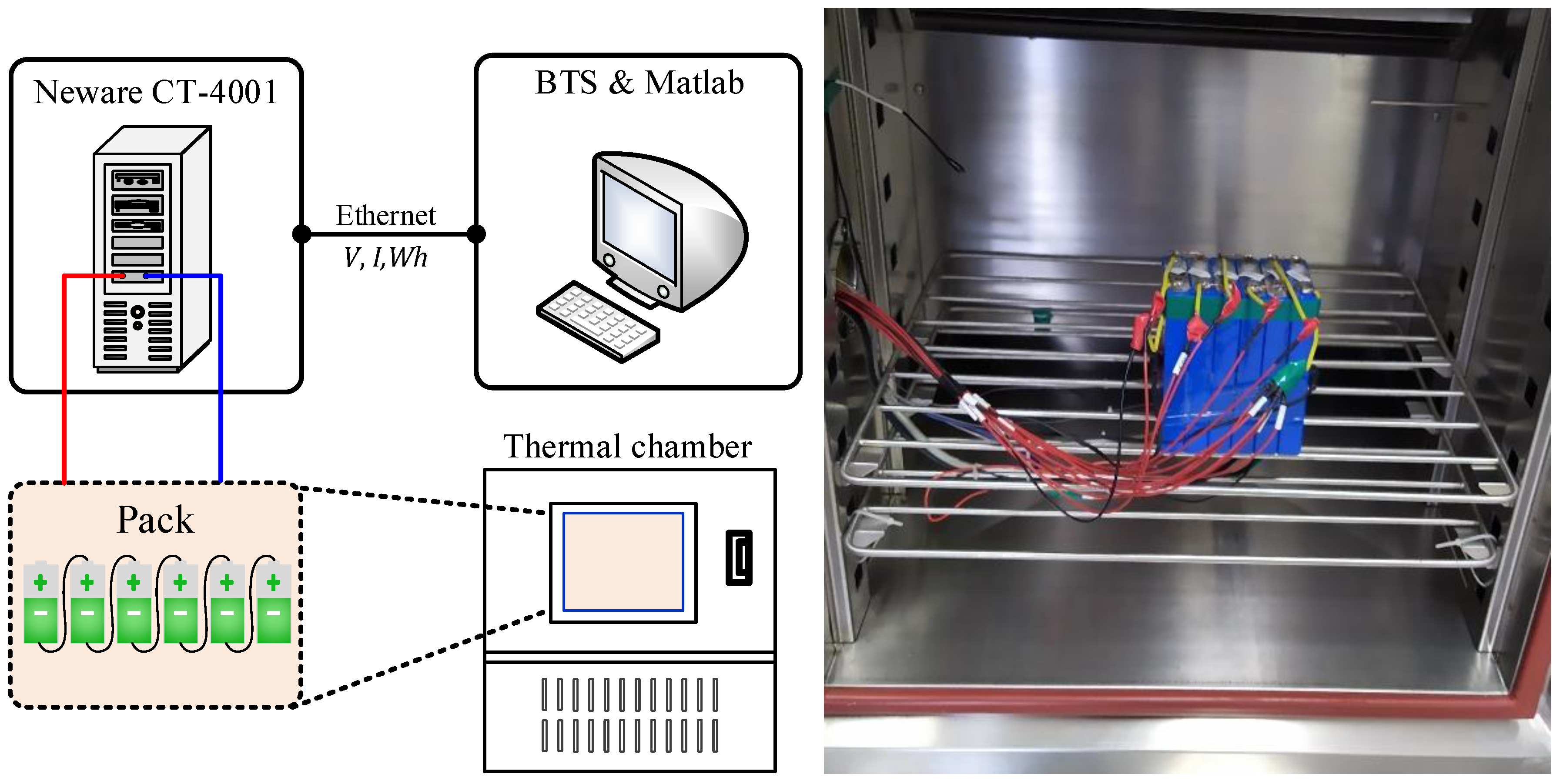
As Figure 1 depicts, the platform consisted of a CT-4001 battery test cabinet (60 V/100 A, 0.02% FSR; NEWARE, Shenzhen, Guangdong, China), a temperature chamber (−20~100 °C; Suyida, Wuxi, Jiangsu, China) and a computer (Thinkpad T430). The tested battery sample was a pack comprising 6 LiFeO₄/graphite batteries (LFPBs) connected in series (nominal voltage of 19.2 V, rated capacity of 20 Ah by 1C (C rate is the magnitude of charge or discharge current with respect to the specified battery’s nominal capacity, e.g., the absolute value of 1C for a 2 Ah battery is 2 A) at 27 °C. In addition, the CT-4001 comes with temperature-sensing ports, since battery temperature is a crucial variable impacting the power [16], and the drop-shaped thermistors are attached to the battery for surface temperature. When calibrated, the maximum static measurement error is mostly less than 0.5 °C during the temperature range concerned in this work (0~60 °C). The PC ran the accompanying BTS software (v3.3.1, NEWARE, Shenzhen, Guangdong, China) and the simulation and prediction scheme was implemented with MATLAB (v2018b, MathWorks, Natick, MA, USA). Considering that some characterization tests can result in irreversible degradation, two packs were used in this work, i.e., B1 was used for model characterization and B2, for method verification. As for data sampling and recording, the current, voltage, and temperature were measured with an interval of 1 s. The commonly adopted constant-current/constant-voltage charging procedure was used to charge the battery. As is known, LFPBs have a flat voltage platform during the dominate SoC range [17], so it is more challenging to estimate and predict the state.

2.1. Characterizations on B1

To determine battery characteristics, a series of calibration tests, including static capacity tests, Coulombic efficiency tests and open circuit voltage (OCV)-SoC tests, were arranged on B1. The $C_n$ and $\eta$ under different conditions of temperature and aging are listed in

Table 1. Calibrated $C_n$ and $\eta$ under different conditions.

	Temp. (°C)	Aging Cycles
		0	200	400	600	800
${\mathit{C}}_{\mathit{n}}$ (Ah)	0	17.64	16.97	16.18	15.21	14.18
	15	18.85	18.3	17.58	16.61	15.58
	30	19.70	19.33	18.48	17.45	16.24
	45	20.73	19.88	19.15	18.30	17.03
$\mathit{\eta }$	0	0.977	0.972	0.968	0.962	0.951
	15	0.985	0.984	0.983	0.972	0.963
	30	0.991	0.991	0.989	0.982	0.971
	45	0.993	0.992	0.988	0.986	0.971

. Along with the aggravation of aging and the decrease of temperature, $C_n$ exhibits obvious attenuation; capacity degradation and temperature decrease show a remarkable influence on $\eta$. The OCV-SoC curves in both directions are acquired and the median curve is adopted. Then, by fitting the acquired points, a function is used to express the OCV-SoC correlation as follows:

$$\begin{array}{c}{U}_{oc}\left(s,C_n\right)={\alpha }_0+{\alpha }_{1}s+{\alpha }_2{s}^2+{\alpha }_3{s}^3+{\alpha }_4/s+{\alpha }_5\mathit{ln}s+{\alpha }_6\mathit{ln}\left(1-s\right)\end{array}$$

(1)

where “s” is shorthand for SoC and the coefficients of ${\alpha }_i$ are listed in

Table 2. Calibrated coefficients of Equation (1).

Parameter	Formulation
${\mathit{\alpha }}_{\mathbf{0}}$	24.84 − 2.39$C_n$ + 0.058$C_n{}^2$
${\mathit{\alpha }}_{\mathbf{1}}$	−51.05 + 5.19$C_n$ − 0.126$C_n{}^2$
${\mathit{\alpha }}_{\mathbf{2}}$	42.05 − 4.32$C_n$ + 0.107$C_n{}^2$
${\mathit{\alpha }}_{\mathbf{3}}$	−13.75 + 1.43$C_n$ − 0.035$C_n{}^2$
${\mathit{\alpha }}_{\mathbf{4}}$	0.574 − 0.055$C_n$ + 0.0012$C_n{}^2$
${\mathit{\alpha }}_{\mathbf{5}}$	11.00 − 1.106$C_n$ + 0.027$C_n{}^2$
${\mathit{\alpha }}_{\mathbf{6}}$	−23.76 + 3.76$C_n$ − 0.198$C_n{}^2$ + 0.0034$C_n{}^3$

. Specifically, $C_n$ is involved as the complementary variable of ${\alpha }_i$ to convert the influence of aging and temperature to a more direct capacity change.

2.2. Verification on B2

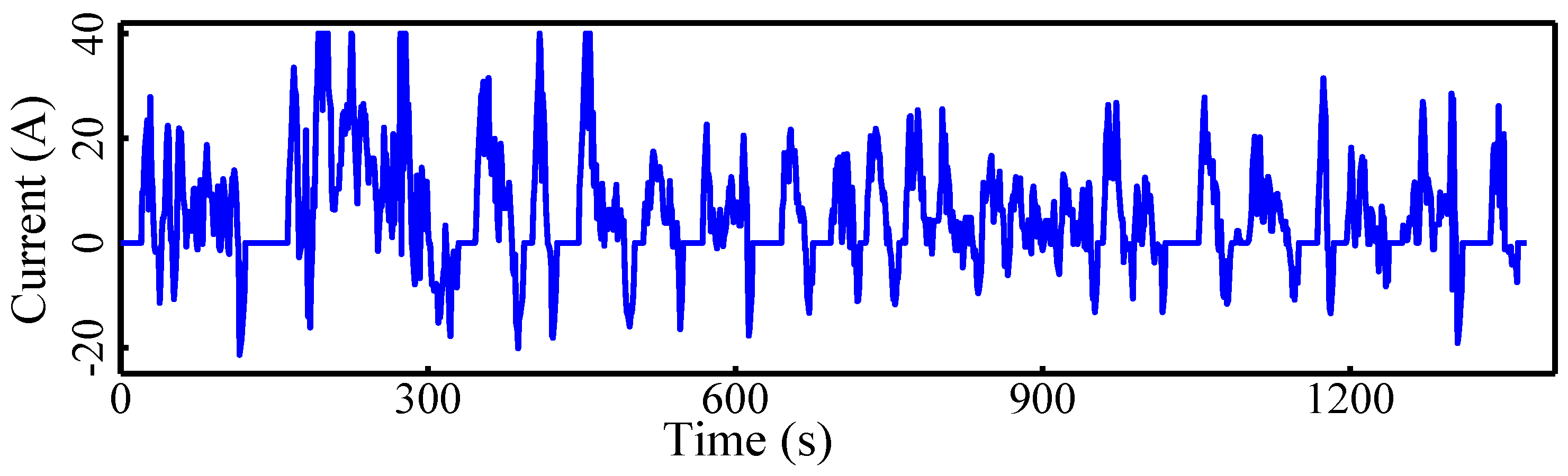
Benefiting from the diverse current rates and frequent charge–discharge switchovers, the federal urban driving schedule (FUDS) has been broadly accepted to verify the performance of state estimating and battery modeling methods. This work uses B2 as the sample to evaluate the constructed SoP predictor subject to the load regime consisting of consecutive FUDS cycles. The example of one FUDS cycle scaled according to the employed battery’s capacity is given in Figure 2.

3. Battery Modeling

3.1. Equivalent Circuit Model

The electrical behaviors of batteries can be effectively imitated by lumped ECMs with reliable accuracy. This work resorts to a first-order ECM to capture LFPB electrical characteristics. As Figure 3 shows,$U_t$ is the battery terminal voltage between the electrodes, $i_L$ means the applied current (>0 as discharging, $0$ as charging), $R_{\Omega }$ represents the internal resistance from solid and liquid phase resistance and component contact resistance, etc., which is separated as $R_{\Omega }^{dch}$ and $R_{\Omega }^{ch}$ for discharging and charging. $R_D//C_D$ determines the transient behavior with a potential of $U_D$. It should be noted that the hysteresis phenomenon of LFPB is non-ignorable and thus a hysteresis potential element of $U_h$ is added. Then, the following equations express the electrical relationships of Figure 3:

$$\{\begin{array}{c}{U}_{D,k+1}=\left(1-\mathbb{E}\right)i_{L,k}{R}_D+\mathbb{E}{U}_{D,k}\\ U_{t,k+1}=U_{oc,k+1}-U_{D,k+1}-i_{L,k+1}{R}_{\Omega }+U_{h,k+1}\end{array}$$

(2)

where $\mathbb{E}=exp\left(-\Delta t/{\tau }_D\right)$, $k$ is the step index, and ${\tau }_D=R_D{C}_D$ is the time constant of mass transportation. In this work, the efficient one-state hysteresis potential model in [18] is used to track $U_h$ as follows:

$$U_{h,k+1}={\mathbb{E}}_{h,\mathrm{k}}{U}_{h,k}-sign\left(i_{L,k}\right)\left(1-{\mathbb{E}}_{h,k}\right){\mathscr{H}}_k$$

(3)

where ${\mathbb{E}}_{h,k}=exp\left(-\left|i_{L,k}\Delta t/{\kappa }_h\right|\right)$, ${\kappa }_h$ is the decaying coefficient, ${\mathscr{H}}_{\mathrm{k}}$ is the shuttle amplitude, and the involved parameters can be identified referring to [19].

3.2. Thermal Model

As long as current flows through the battery, there is heat generated due to the thermogenesis effect [20]. Thereafter, a portion of the generated heat is dissipated by convection and the left portion results in the elevation of temperature. Assuming the battery as a mass point without temperature gradient, the dominated thermal effects can be written as follows [21]:

$$\underset{Heat generation}{\underbrace{{i_L}^2{R}_{\Omega }+\frac{{\left(\Delta E-i_L{R}_{\Omega }\right)}^2}{R_D}}}=\underset{Battery heat variation}{\underbrace{m{c}_p\frac{d{T}_s}{dt}}}+\underset{Heat dissipation}{\underbrace{h_c\varphi \left(T_s-T_a\right)}}$$

(4)

where $\Delta E=U_{oc}-U_t+U_h.$ Rearranging Equation (4), we obtain the following:

$${\kappa }_1\dot{T_s}=i_L{}^2{R}_{\Omega }+\frac{{\left(\Delta E-i_L{R}_{\Omega }\right)}^2}{R_D}-{\kappa }_2{T}_s+{\kappa }_2{T}_a$$

(5)

where ${\kappa }_1= m{c}_p$,${\kappa }_2=h_c\varphi$. Further transforming Equation (4), we obtain the following:

$$\dot{T_s}=-\frac{{\kappa }_2}{{\kappa }_1}{T}_s+\frac{{\kappa }_2}{{\kappa }_1}\left(\frac{i_L{}^2{R}_{\Omega }}{{\kappa }_2}+\frac{{\left(\Delta E-i_L{R}_{\Omega }\right)}^2}{R_D{\kappa }_2}+T_a\right).$$

(6)

That is,

$$\dot{T_s}=-\frac{{\kappa }_2}{{\kappa }_1}{T}_s+\frac{{\kappa }_2}{{\kappa }_1}M$$

(7)

where $M=i_L{}^2{R}_{\Omega }/{\kappa }_2+{\left(\Delta E-i_L{R}_{\Omega }\right)}^2/R_D{\kappa }_2+T_a$. Then, Equation (6) can be converted into a recursive discrete form to govern the battery temperature evolution process as follows:

$$T_{s,k+1}={\mathbb{E}}_T{T}_{s,k}+\left(1-{\mathbb{E}}_T\right)M_k$$

(8)

where ${\mathbb{E}}_T=exp\left(-{\kappa }_2\Delta t/{\kappa }_1\right)$.

3.3. On-Line Parameterization of ECM

Inside Li-ion batteries, various physico-chemical reactions are present that have a distinct dependency on temperature, load, aging, SoC, etc. [22,23]. Therefore, fixed model parameters are unrealistic, and many on-line and off-line methods are reported for ECM parameterization. Among them, the separate estimation of states and parameters can obviously intensify the computational burden, whereas joint estimators cause cross-interference problems. Here, the low sophisticated recursion algorithm as described in [24] was used to update the parameters ${\theta }_{LMS}={\left[\begin{array}{ccc}{R}_{\Omega }^{ch}& R_{\Omega }^{dch}& R_D\end{array}\right]}^T$, whereby the defects from high computational cost and cross-interference can be avoided.

4. SoC Estimation and SoP Prediction

4.1. UPF-Based SoC Estimation

The extended kalman filter (EKF) has been extensively exploited for system state estimation because of its capability in handling system nonlinearities and noises. However, the first-order truncation approximation of the Taylor expansion makes the estimator suffer obvious degradation in the case of severe nonlinearities. Moreover, the assumption of Gaussian white noises and the requirement of accurate model are impractical. From the view of probability, a particle filter (PF) can give remarkable immunity to nonlinearities and noise variations while the high computational overhead is intractable. Accordingly, by applying the unscented transformation on PF, a new form of UPF gives the desirable trade-off between accuracy and complexity. In UPF, the resampling operation is executed involving new measurements and the posterior probability is obtained including the newest observations; the number of particles is thereby effectively restrained [25].

For a nonlinear discrete-time system, we have the following:

$$\{\begin{array}{c}{x}_{k+1}=f\left(x_k,u_k,{\omega }_k\right)\\ y_{k+1}=g\left(x_{k+1},u_{k+1},{\nu }_{k+1}\right)\end{array}$$

(9)

where $x_k$, $y_k$, and $u_k$ mean system state, output, and input, respectively, ${\omega }_k$ and ${\nu }_k$ are independent Gaussian white noises with covariances of $R_{\omega }$ and $R_{\nu }$, respectively, and the covariance of $x_k$ is $P_{x,k}$. $x_k$ is augmented as $x_k^a={\left[\begin{array}{ccc}{x}_k^T& {\omega }_k^T& v_k^T\end{array}\right]}^T$ with the covariance matrix augmented as $P_k^a=diag\left(P_{x,k},R_{\omega },R_{\nu }\right)$. Then, the estimation of $x_k$ can be implemented by recursing the UPF algorithm, as detailed in [26], using periodically updated $u_{1, \dots , k+1}$ and $y_{1, \dots , k+1}$.

In this work, the battery SoC evolves as follows:

$$s_{k+1}=s_k-i_{L,k}\eta \Delta t/C_n$$

(10)

where $i_{L,k}$ is the load current, $\Delta t$ is the step interval, $C_n$ is the maximum available capacity under the specified condition. Combining Equations (1)–(3) and Equation (10), the state–space expression with SoC, $U_D$ and $U_h$ as internal states can be extracted as follows:

$$\{\begin{array}{c}{x}_k={\left[\begin{array}{ccc}{s}_k& U_{D,k}& U_{h,k}\end{array}\right]}^T \\ u_k={\left[\begin{array}{cc}{i}_{L,k}& sign\left(i_{L,k}\right){\mathscr{H}}_k\end{array}\right]}^T\\ y_k=U_{t,k}=U_{oc,k}-U_{D,k}-i_{L,k}{R}_{\Omega }+U_{h,k}\\ A=diag\left({\left[\begin{array}{c}1\\ \mathbb{E}\\ {\mathbb{E}}_h\end{array}\right]}^T\right), B=\left[\begin{array}{cc}-\eta \Delta t/C_n& 0\\ \left(1-\mathbb{E}\right)R_D& 0\\ 0& -\left(1-{\mathbb{E}}_h\right)\end{array}\right]\end{array}$$

(11)

Afterward, the battery SoC can be estimated by applying the introduced UPF algorithm on the system as Equation (11) describes [26].

4.2. Peak Current Estimation

To optimize energy efficiency and prolong battery life, some operating recommendations should be complied with. For example, battery temperature should not be out of the safe range, and the SoC should be kept within the high-efficiency range, especially for hybrid EVs. The above sections give ECM parameters and the SoC; the SoP is thus predictable according to the prescribed constraints concerning terminal voltage, affordable current, preferable SoC, and temperature ranges. In this section, the SoP is predicted by the following steps:

• First, the peak currents limited by the three constraints on terminal voltage, SoC, and working temperature are estimated;
• Then, the obtained three pairs of peak currents, along with the current limits, are compared and the final peak currents are determined as the most conservative ones;
• With the currents obtained in the preceding step, the corresponding terminal voltages are derived, and thereby the power capabilities can be given.

4.2.1. Peak Current by Voltage Limits

Let us assume that the current during $\left[\begin{array}{cc}k\Delta t& \left(k+1\right)\Delta t\end{array}\right]$ is fixed, then the $U_t$ at $t=\left(k+1\right)\Delta t$ is as follows:

$$\begin{array}{c}{U}_{t,k+1}=U_{oc,k+1}-\mathbb{E}{U}_{D,k}+U_{h,k+1}-\left(R_{\Omega }+\left(1-\mathbb{E}\right)R_D\right)i_{L,k}\end{array}$$

(12)

where $U_{h,k+1}$ is the hysteresis potential, which is significant for LFPBs and modeled by Equation (3).

Referring to the allowable terminal voltages ($U_{t,max}$ and $U_{t,min}$), usually provided by the manufacturer, the peak currents can be deduced as follows:

$$\{\begin{array}{c}\begin{array}{c}{U}_{t,max}=U_{h,k+1}-\left(R_{\Omega }+\left(1-\mathbb{E}\right)R_D\right)I_{min}^{c,v}+U_{oc,k+1}-\mathbb{E}{U}_{D,k}\end{array}\\ \begin{array}{c}{U}_{t,min}=U_{h,k+1}-\left(R_{\Omega }+\left(1-\mathbb{E}\right)R_D\right)I_{max}^{d,v}+U_{oc,k+1}-\mathbb{E}{U}_{D,k}\end{array}\end{array}$$

(13)

where $I_{min}^{c,v}$ and $I_{max}^{d,v}$ represent extreme currents by the constraints of $U_{t,max}$ and $U_{t,min}$, respectively. It is noteworthy to emphasize that $I_{min}^{c,v}$ means the charge current with the maximum absolute value because the charging current is defined previously as negative. $I_{min}^{c,v}$/$I_{max}^{d,v}$ cannot be obtained by simply rearranging Equation (13) because $U_{oc}$ is nonlinearly correlated with SoC, which is the function of $I_{min}^{c,v}$/$I_{max}^{d,v}$ as well. Herein, the Taylor series expansion is used to decompose Equation (1) as follows:

$$\begin{array}{l}{U}_{oc,k+1}=U_{oc}\left(s_k-\frac{i_{L,k}\eta \Delta t}{C_n}\right) =U_{oc}\left(s_k\right)-\frac{i_{L,k}\eta \Delta t}{C_n}{\frac{\partial U_{oc}\left(s\right)}{\partial s}|}_{s=s_k}+{ℛ}_1\left(s_k,\frac{i_{L,k}\eta \Delta t}{C_n}\right)\hfill \\ \hfill \end{array}$$

(14)

where ${ℛ}_1(·)$ is the residual of the first-order truncation and is negligible, not making significant deviation on $U_{oc}$ during the small time span of $\Delta \mathrm{t}$ [10]. Then, combining Equations (13) and (14), the allowable peak current under voltage constraints can be derived as follows:

$$\{\begin{array}{c}{I}_{max}^{d,u}=\frac{U_{oc}\left(s_k\right)-\mathbb{E}{U}_{D,k}-U_{t,min}+U_{h,k+1}}{\frac{\eta \Delta t}{C_n}{\frac{\partial U_{oc}\left(s\right)}{\partial s}|}_{s=s_k}+\left(1-\mathbb{E}\right)R_D+R_{\Omega }}\\ I_{min}^{c,u}=\frac{U_{oc}\left(s_k\right)-\mathbb{E}{U}_{D,k}-U_{t,max}+U_{h,k+1}}{\frac{\eta \Delta t}{C_n}{\frac{\partial U_{oc}\left(s\right)}{\partial s}|}_{s=s_k}+\left(1-\mathbb{E}\right)R_D+R_{\Omega }}\end{array}$$

(15)

4.2.2. Peak Currents by SoC Limits

The sustained current applied on the battery should also ensure that the SoC stays in the optimal working range across the future time interval $\mathsf{\Delta }\mathrm{t}$. Given the SoC limits of $s_{max}$ and $s_{min}$, the peak current can be deduced as follows:

$$\{\begin{array}{c}{I}_{min}^{c,s}=\frac{s_k-s_{max}}{\eta \Delta t}{C}_n\\ I_{max}^{d,s}=\frac{s_k-s_{min}}{\eta \Delta t}{C}_n\end{array}$$

(16)

where $I_{min}^{c,s}$ and $I_{max}^{d,s}$ are the extreme loads subject to $s_{max}$ and $s_{min}$.

4.2.3. Peak Currents by Temperature Limit

In the case of high surrounding temperature, the battery temperature should always be monitored to avert hazardous thermal damage. Regarding $I_{max}^T$ as the independent variable, the solution can be deduced from Equation (7) as follows:

$$I_{max}^T{}^2{R}_{\Omega }\left(R_D+R_{\Omega }\right)-2I_{max}^T\Delta E{R}_{\Omega }+\left(\Delta E^2-\Lambda R_D{\kappa }_2\right)=0$$

(17)

where $\Lambda =\left(T_{max}-{\mathbb{E}}_T{T}_{s,k}\right)/\left(1-{\mathbb{E}}_T\right)-T_a$, $T_{max}$ is the maximum working temperature and $I_{max}^T$ is the corresponding extreme load current. During Δ$\mathrm{t}$, the slow-varying $U_{oc}$ has negligible influence on battery temperature evolution, so $U_{oc}$ is deemed as invariable and derived by Equation (1). Afterward, $I_{max}^T$. is the solution of Equation (17) as follows:

$$I_{max}^T=\frac{-b-{\left(b^2-4ac\right)}^{1/2}}{2a}$$

(18)

where $a=R_{\Omega }\left(R_D+R_{\Omega }\right)$, $b=-2\Delta E{R}_{\Omega }$, $c=\Delta E^2-\Lambda R_D{\kappa }_2$.

4.2.4. Current Capabilities by all the Limits

Comparing the previously derived current values, the synthesized global currents limited by all the prescribed constraints on the four aspects of constraints can be obtained as follows:

$$\{\begin{array}{c}{ℐ}_{max}^d=min\left(I_{max},I_{max}^{d,u},,I_{max}^{d,s},I_{max}^T\right)\\ {ℐ}_{min}^c=max\left(I_{min},I_{min}^{c,u}, I_{min}^{c,s},-I_{max}^T\right)\end{array}$$

(19)

where $I_{max}$ and $I_{min}$ are manufacturer-provided current limits and ${ℐ}_{max}^d$ and ${ℐ}_{min}^c$ are the maximum discharging and minimum charging currents, respectively.

4.3. SoP Prediction

Based on the retained ${ℐ}_{max}^d$ and ${ℐ}_{min}^c$ in Equation (19), the corresponding $U_t$ can be obtained from Equations (13) and (14) as follows:

$$\{\begin{array}{c}{U}_{t,k+1}^{c,s}=U_{oc}\left(s_k\right)-\mathbb{E}{U}_{D,k}+U_{h,k+1}-{ℐ}_{min}^c\left(\frac{\eta \Delta t}{C_n}{\frac{\partial U_{oc}\left(s\right)}{\partial s}|}_{s=s_k}+R_{\Omega }+\left(1-\mathbb{E}\right)R_D\right)\\ U_{t,k+1}^{d,s}=U_{oc}\left(s_k\right)-\mathbb{E}{U}_{D,k}+U_{h,k+1}-{ℐ}_{max}^d\left(\frac{\eta \Delta t}{C_n}{\frac{\partial U_{oc}\left(s\right)}{\partial s}|}_{s=s_k}+R_{\Omega }+\left(1-\mathbb{E}\right)R_D\right)\end{array}$$

(20)

Finally, the continuous powers across the future time span of $\mathsf{\Delta }\mathrm{t}$ restricted by multiple constraints is determined as follows:

$$\{\begin{array}{c}{\mathcal{P}}_{max}^d=U_{t,k+1}^{d,s}{ℐ}_{max}^d\\ {\mathcal{P}}_{min}^d=U_{t,k+1}^{c,s}{ℐ}_{min}^c\end{array}$$

(21)

where ${\mathcal{P}}_{max}^{dc}$ and ${\mathcal{P}}_{max}^c$ are the available powers subject to all the constraints on $U_{t,max}$, $U_{t,min}$, $s_{max}$, $s_{min}$, $T_{max}$, $I_{max}$ and $I_{min}$.

5. Experimental Results and Analysis

To examine the proposed SoP prediction methodology, experimental verifications under various conditions, including different aging states, temperatures, and loads, were carried out on B2. Since aging is an irreversible process, the experiments were arranged according to the principle of from fresh to aged. During the experiments, the $C_n$ and $\eta$ were obtained by quadratic interpolation on the results listed in Table 1. In addition, different prediction time horizons were utilized to assess power persisting capability for different driving scenarios.

Table 3. Working constraints of the investigated battery pack.

Constraint	Value
Voltage (${\mathit{U}}_{\mathit{t},\mathit{m}\mathit{a}\mathit{x}}$, ${\mathit{U}}_{\mathit{t},\mathit{m}\mathit{i}\mathit{n}}$)	21.6 $\mathrm{V}$, 15 $\mathrm{V}$
SoC ($S_{\mathit{m}\mathit{a}\mathit{x}}$, $S_{\mathit{m}\mathit{i}\mathit{n}}$)	0.9, 0.1
Current (${\mathit{I}}_{\mathit{m}\mathit{a}\mathit{x}}$, ${\mathit{I}}_{\mathit{m}\mathit{i}\mathit{n}}$)	100 A, −80 A
Temperature (${\mathit{T}}_{\mathit{m}\mathit{a}\mathit{x}}$)	50 °C

lists the design and operation limits of the LFPB pack and

Table 4. Parameters of the designed thermal model.

Parameter	Value
Heat capacity (${\mathit{c}}_{\mathit{p}}$)	988 ${\mathrm{Jkg}}^{-1}{\mathrm{K}}^{-1}$
Convection coefficient (${\mathit{h}}_{\mathit{c}}$)	4.11 ${\mathrm{Wm}}^{-2}{\mathrm{K}}^{-1}$
Effective surface area (pack) ($\mathit{\varphi }$)	$8.30$e−2${\mathrm{m}}^2$
Mass (pack) ($\mathit{m}$)	3 kg

tabulates the parameters of the TEM. As a comparison, the widely used PNGV-HPPC method [8] is also used to give predictions without considering hysteresis effect, time horizon, and polarization relaxation. Note that, in [8], ECM parameters are determined in advance and then interpolated for on-line applications. In this work, the PNGV-HPPC method was adapted: the ($R_{\Omega }^{ch}$, $R_{\Omega }^{dch}$, $R_D$) are also on-line identified as Section 3.3 presents.

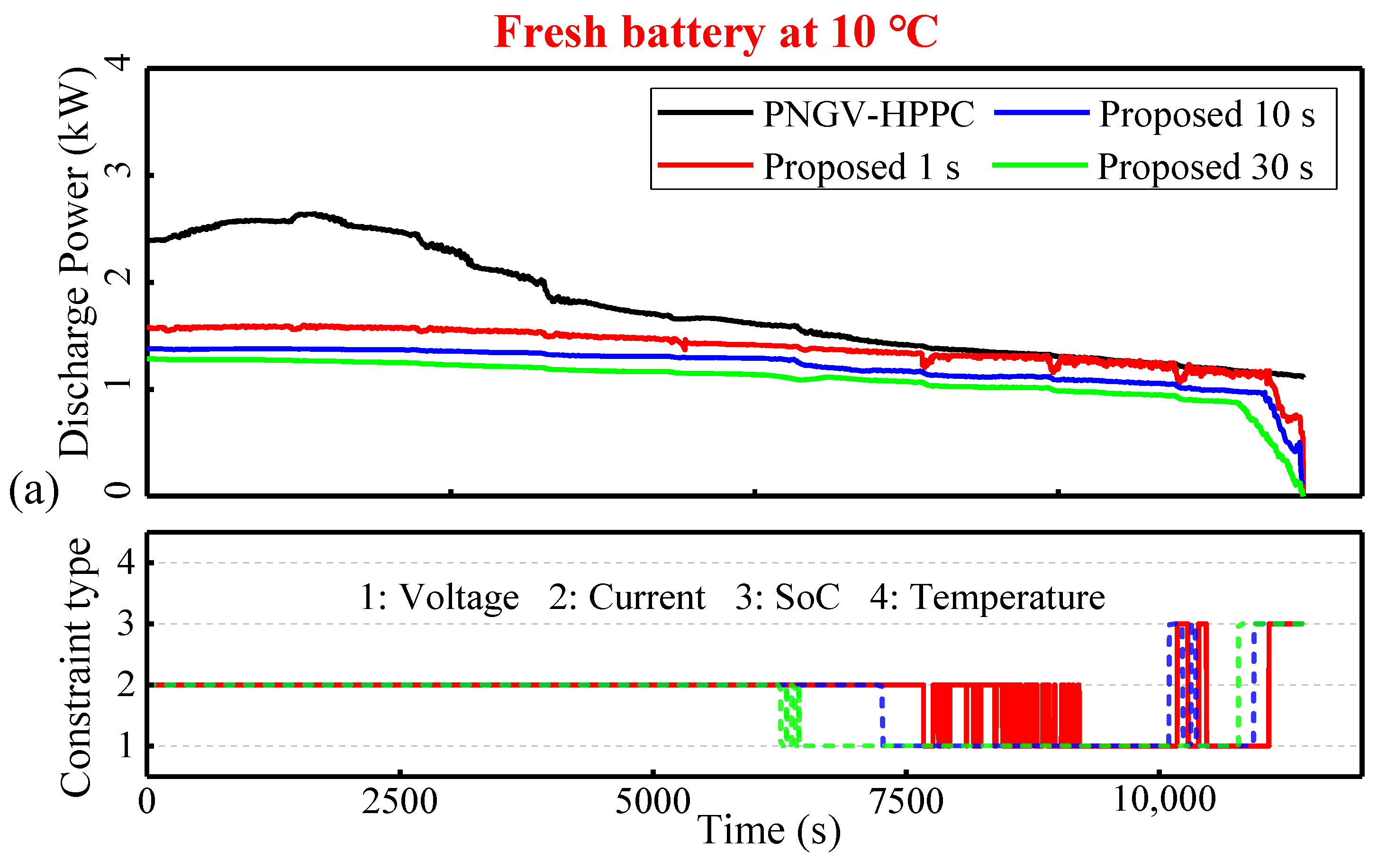
5.1. SoP Prediction on a Fresh Battery at 10 °C

First, an experiment on a fresh B2 pack at 10 °C is presented as a preliminary verification. As Figure 4 illustrates, each constraint (voltage, current, SoC) occupies some entry-into-force times across the whole experiment, except the constraint of temperature. Although low temperature results in a larger internal resistance and thus more heat generation, low ambient temperature also brings about considerable heat dissipation, so temperature constraint is always at an invalid state. From Figure 4a, the former half-phase from beginning to about 5000 s, the PNGV-HPPC method gives apparently stronger power outputs with significant fluctuations especially in the discharging direction; meanwhile, the proposed method delivers more stable SoP because the dominated constraint is current that is ignored in PNGV-HPPC. The PNGV-HPPC discharge power curve characterizes a first-rise-then-descend shape during t = 0–3500 s, possibly ascribing to the similar change of $R_{\Omega }^{dch}$. Moreover, the charging powers contain more spikes as compared to the discharging because the charging resistance $R_{\Omega }^{ch}$ is more sensitive to load dynamics. Another reasonable phenomenon are the steep falls around both the beginning of charging and the end of discharging where, for example, a small charge amount can overbrim the battery beyond the SoC constraint for charging, and vice versa. In summary, the PNGV-HPPC method is less reliable because it has an exclusive dependence on terminal voltage, while other involved constraints also play critical roles in limiting the power in the proposed method.

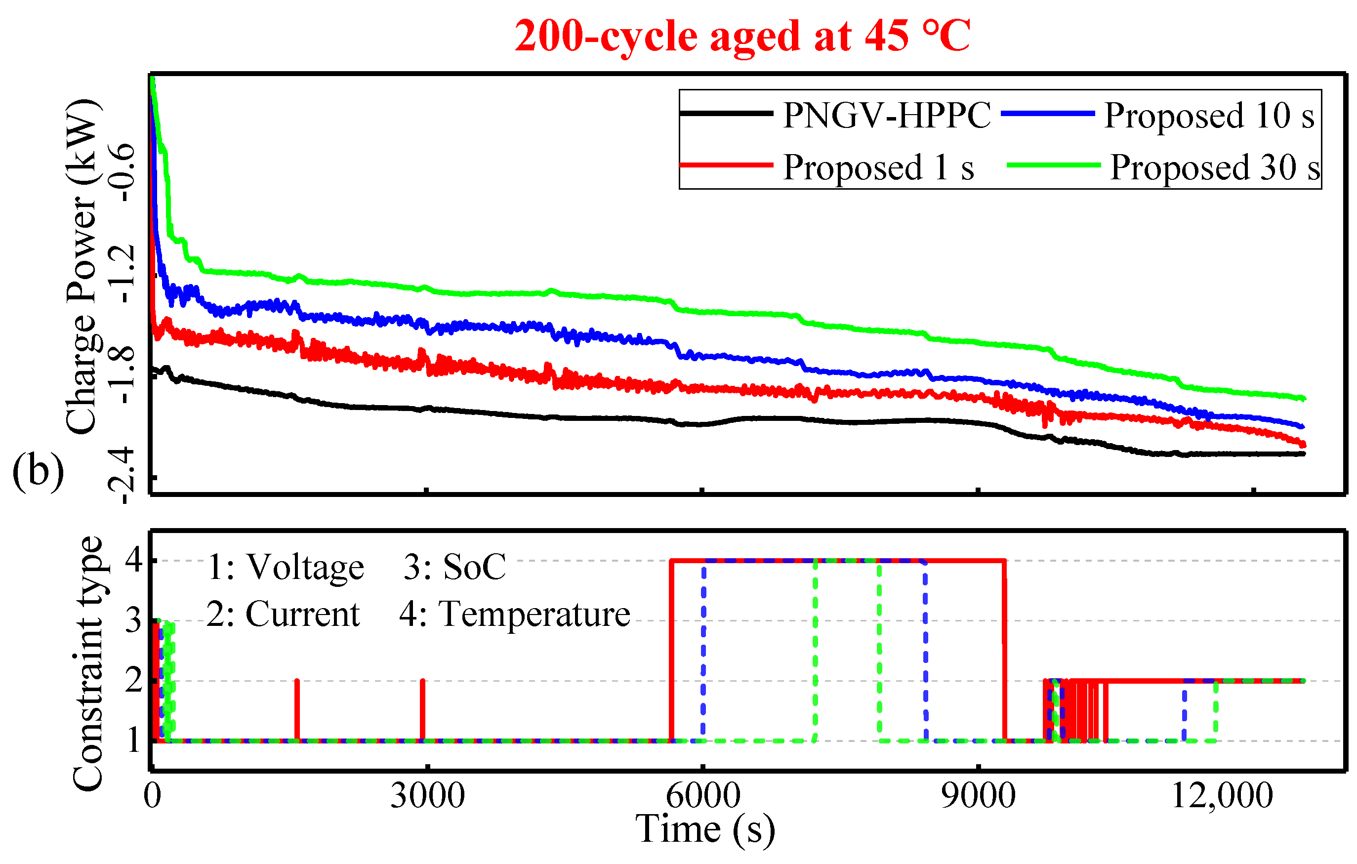
5.2. SoP Prediction on 200-Cycle Aged Battery at 45 °C

The aging of batteries is inevitable due to electrolyte dry up or any other material decomposition, resulting in capacity shrink and resistance increase. Therefore, the aging factor should also be considered. To emphasize the most characteristic contribution on thermal consideration, an experiment on a 200-cycle aged B2 at 45 °C, which is close to the prescribed temperature constraint, was carried out. Figure 5 presents the results and verifies the efficiency of temperature constraint.

As can be seen in Figure 5a, the PNGV-HPPC again gives significant overestimation across the first half-time. Remarkably, the temperature threshold of 50 °C is reached by all three predicting horizons, namely 1 s, 10 s, and 30 s, of the proposed method. The ambient 45 °C greatly slows down the heat dissipation, so accumulated heat can easily exceed the temperature bound. As the horizon extends, the duration that the temperature constraint is activated shrinks. As restored charge consumes, the gradually weakened battery potential causes the decline of discharge power and the reduction of the generated heat. Therefore, the temperature warning is dispelled and the constraints of voltage and current return as being dominant. Thereafter, the predictions of 1 s and PNGV-HPPC start a progressive convergence because they are both subject to voltage constraint, and the inclusion of the 1 s horizon only creates a few differences from the instantaneous mechanism of the PNGV-HPPC. Afterward, the SoC constraint takes effect and the proposed method behaves in a descending trend, whereas the PNGV-HPPC power keeps relatively stable. Specifically, approaching the exhaustion phase, there are springbacks in the 1 s and 10 s predictions that come from the current pulse of FUDS. Overall, the 1 s curve presents more violent fluctuations relative to the PNGV-HPPC curve because the former can deal with transient dynamics by the incorporated features of RC pair and hysteresis.

For the charging cases in Figure 5b, the PNGV-HPPC method again delivers stronger powers than the proposed method, while the deviations are not so obvious. As the horizon narrows from 30 s down to 1 s, power oscillations also intensify. This can be explained by the fact that a shorter interval can acquire more load details, which, however, are omitted by longer time spans. Surely, the temperature constraint restricts the power for a long time as well as in the discharging cases, except for some horizontal displacement, i.e., the temperature-in-charge times in the charging and discharging cases do not precisely align. This can be attributed to the asynchronized changing of the $R_{\Omega }^{dch}$ and $R_{\Omega }^{ch}$. Then, in the final phase, current constraint takes effect in the proposed method and, subsequently, the PNGV-HPPC power behaves in a diverging trend.

In fact, the constraints in Table 3 are given as instantaneous working limitations. Therefore, the SoP of the 1 s horizon is probably underestimated because the acceptable currents for 1 s are normally higher than those for 10 s. Similarly, the 30 s SoP prediction is probably overestimated. Predicting continuous powers according to these restrictions may cause damage to the battery. Nevertheless, to form a consistent comparison basis, these restrictions were still utilized by the two methods in this work. Therefore, the powers used by the proposed method are probably overestimated because the allowable constraints are normally lower than in the instantaneous cases.

5.3. SoP Predicted at Different Temperatures and Aging States

An EV-mounted battery system inevitably suffers aging, so the capacity and power capability will gradually degrade. Besides aging, temperature also imposes significant impacts on battery performance [27,28,29]. Therefore, it is necessary to examine the predictor at different aging and temperature conditions.

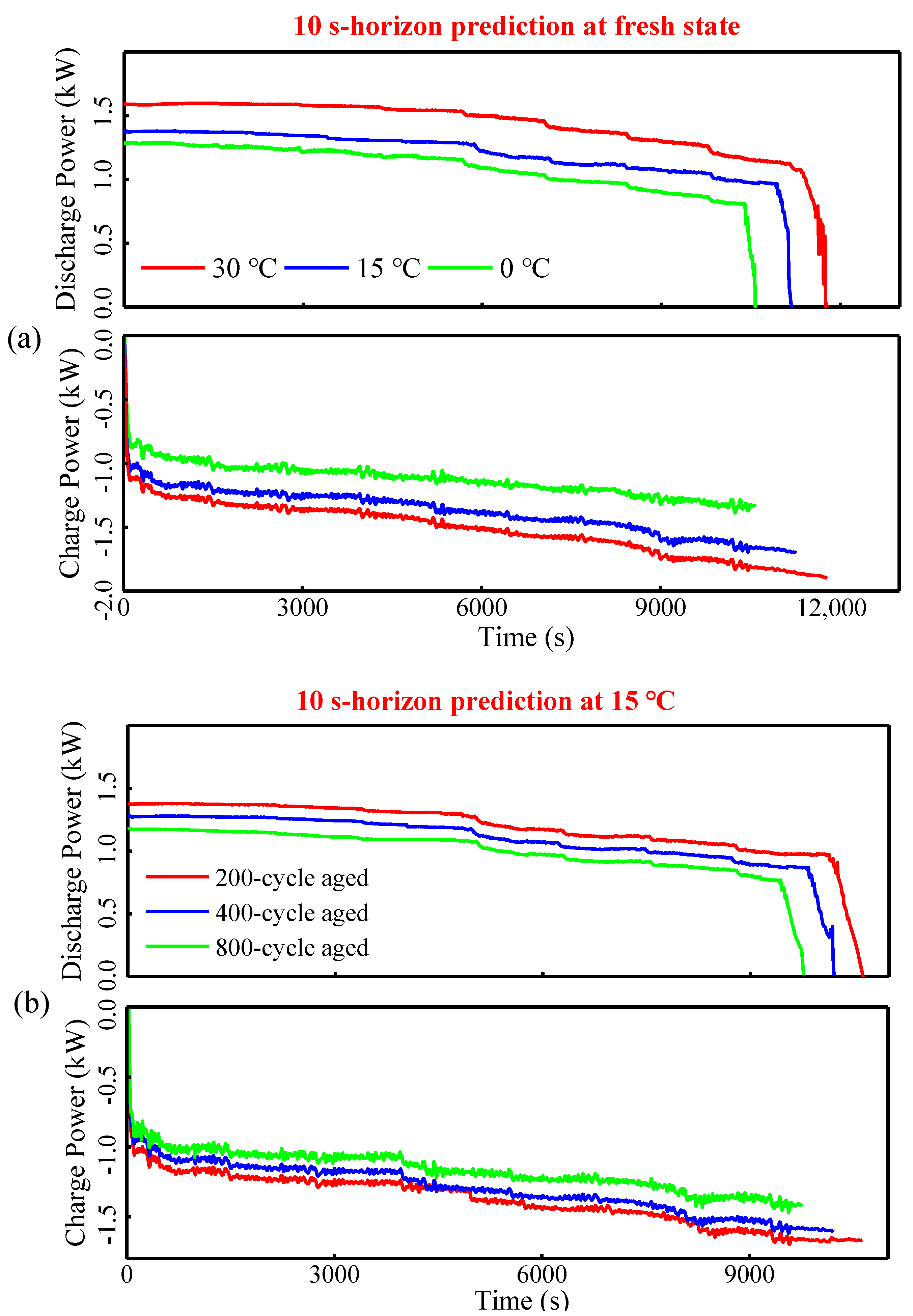
Here, 10 s powers on fresh B2 at different temperatures are outlined in Figure 6a. As expected, temperature increase can apparently but nonlinearly influence battery power capability. A higher temperature elevates the available power, which can be partially ascribed to the reduction of internal resistance. In addition, a higher temperature brings about a larger capacity; therefore, at the same SoC, more charge throughputs are available and thus contribute to the strength of power.

Figure 6b presents 10 s powers at different aging states on B2 at 15 °C. The discharging power is appreciably reduced as the aging level aggravates, which causes increasing internal resistance. The charging power tends to weaken in smaller magnitudes than the discharging power, which suggests that aging incurs more obvious influences on $R_{\Omega }^{dch}$, while $R_{\Omega }^{ch}$ does not deteriorate in sync.

Finally, to provide an intuitive view, the average powers at different aging and temperature states are presented in Figure 7. It is highlighted that degradation and low temperature have adverse effects on discharging powers while aging is relatively insignificant regarding the charging powers, which is in agreement with above analysis.

6. Discussion and Conclusions

To provide useful information on battery power capability, this paper enhanced a first-order ECM using on-line identified parameters and incorporating a hysteresis element to track battery internal potential more closely, whereby a UPF-based SoC estimator was designed. In addition, to include temperature consideration, a TEM was also derived and battery temperature could be forecasted. Afterward, a model-based power capability prediction method was proposed subject to multiple working constraints. Finally, experimental verifications were arranged on an iron-based Li-ion battery pack excited by highly dynamic FUDS load aimed at different time horizons, aging states, and temperatures. Results show aging and temperature exert pronounced impacts on the available powers. Alongside the intensification of degradation and the decrease of temperature, powers were weakened to different degrees. Owing to the ECM and TEM elaborated for this study, which are critical to sensing different constraints, the proposed method can predict powers with more credibility in contrast to the generally used HPPC method.

References

- Reddy, M.V.; Mauger, A.; Julien, C.M.; Paolella, A.; Zaghib, K. Brief history of early lithium-battery development. Materials 2020, 13, 1884. [Google Scholar] [CrossRef] [PubMed] [Green Version]
- Reddy, M.V.; Julien, C.M.; Mauger, A.; Zaghib, K. Sulfide and oxide inorganic solid electrolytes for all-solid-state li batteries: A review. Nanomaterials 2020, 10, 1606. [Google Scholar] [CrossRef] [PubMed]
- Hu, X.; Feng, F.; Liu, K.; Zhang, L.; Xie, J.; Liu, B. State estimation for advanced battery management: Key challenges and future trends. Renew. Sustain. Energy Rev. 2019, 114, 109334. [Google Scholar] [CrossRef]
- Zhang, X.; Wang, Y.; Wu, J.; Chen, Z. A novel method for lithium-ion battery state of energy and state of power estimation based on multi-time-scale filter. Appl. Energy 2018, 21, 442–451. [Google Scholar] [CrossRef]
- Dong, G.; Wei, J.; Chen, Z. Kalman filter for onboard state of charge estimation and peak power capability analysis of lithium-ion batteries. J. Power Source 2016, 328, 615–626. [Google Scholar] [CrossRef]
- Xiong, R.; Sun, F.; He, H.; Nguyen, T.D. A data-driven adaptive state of charge and power capability joint estimator of lithium-ion polymer battery used in electric vehicles. Energy 2013, 63, 295–308. [Google Scholar] [CrossRef]
- Duong, T.Q. USABC and PNGV test procedures. J. Power Sources 2000, 89, 244–248. [Google Scholar] [CrossRef]
- Plett, G.L. High-performance battery-pack power estimation using a dynamic cell model. IEEE Trans. Veh. Technol. 2004, 53, 1586–1593. [Google Scholar] [CrossRef] [Green Version]
- Sun, F.; Xiong, R.; He, H.; Li, W.; Aussems, J.E.E. Model-based dynamic multi-parameter method for peak power estimation of lithium-ion batteries. Appl. Energy 2012, 96, 378–386. [Google Scholar] [CrossRef]
- Xiong, R.; He, H.; Sun, F.; Liu, X.; Liu, Z. Model-based state of charge and peak power capability joint estimation of lithium-ion battery in plug-in hybrid electric vehicles. J. Power Sources 2013, 229, 159–169. [Google Scholar] [CrossRef]
- Hu, X.; Xu, L.; Lin, X.; Pecht, M. Battery lifetime prognostics. Joule 2020, 4, 310–346. [Google Scholar] [CrossRef]
- Feng, X.; Ouyang, M.; Liu, X.; Lu, L.; Xia, Y.; He, X. Thermal runaway mechanism of lithium ion battery for electric vehicles: A review. Energy Storage Mater. 2018, 10, 246–267. [Google Scholar] [CrossRef]
- Panchal, S.; Gudlanarva, K.; Tran, M.K.; Fraser, R.; Fowler, M. High reynold’s number turbulent model for micro-channel cold plate using reverse engineering approach for water-cooled battery in electric vehicles. Energies 2020, 13, 1638. [Google Scholar] [CrossRef] [Green Version]
- Panchal, S.; Mathewson, S.; Fraser, R.; Culham, R.; Fowler, M. Measurement of temperature gradient (dt/dy) and temperature response (dt/dt) of a prismatic lithium-ion pouch cell with lifepo4 cathode material. SAE Tech. Pap. 2017. [Google Scholar] [CrossRef]
- Patil, M.S.; Seo, J.H.; Panchal, S.; Jee, S.W.; Lee, M.Y. Investigation on thermal performance of water-cooled Li-ion pouch cell and pack at high discharge rate with U-turn type microchannel cold plate. Int. J. Heat Mass Trans. 2020, 155, 119728. [Google Scholar] [CrossRef]
- Tang, X.; Wang, Y.; Yao, K.; He, Z.; Gao, F. Model migration based battery power capability evaluation considering uncertainties of temperature and aging. J. Power Sources 2019, 440, 227141. [Google Scholar] [CrossRef]
- Rao, R.P.; Reddy, M.V.; Adams, S.; Chowdari, B.V.R. Preparation, temperature dependent structural, molecular dynamics simulations studies and electrochemical properties of LiFePO4. Mater. Res. Bull. 2015, 66, 71–75. [Google Scholar] [CrossRef]
- Plett, G.L. Extended Kalman filtering for battery management systems of LiPB-based HEV battery packs: Part 2. Modeling and identification. J. Power Sources 2004, 134, 262–276. [Google Scholar] [CrossRef]
- Zhang, C.; Li, K.; Pei, L.; Zhu, C. An integrated approach for real-time model-based state-of-charge estimation of lithium-ion batteries. J. Power Sources 2015, 283, 24–36. [Google Scholar] [CrossRef] [Green Version]
- Hu, X.; Liu, W.; Lin, X.; Xie, Y. A comparative study of control-oriented thermal models for cylindrical Li-ion batteries. IEEE Trans. Transp. Electr. 2019, 5, 1237–1253. [Google Scholar] [CrossRef]
- Gao, L.; Liu, S.; Dougal, R.A. Dynamic lithium-ion battery model for system simulation. IEEE Trans. Compon. Pack Technol. 2002, 25, 495–505. [Google Scholar] [CrossRef] [Green Version]
- Huang, D.; Chen, Z.; Zheng, C.; Li, H. A model-based state-of-charge estimation method for series-connected lithium-ion battery pack considering fast-varying cell temperature. Energy 2019, 185, 847–861. [Google Scholar] [CrossRef]
- Tang, X.; Wang, Y.; Zou, C.; Yao, K.; Xia, Y.; Gao, F. A novel framework for Lithium-ion battery modeling considering uncertainties of temperature and aging. Energy Convers. Manag. 2019, 180, 162–170. [Google Scholar] [CrossRef]
- Xie, J.; Ma, J.; Bai, K. State-of-charge estimators considering temperature effect, hysteresis potential, and thermal evolution for LiFePO4 batteries. Int. J. Energy Res. 2018, 42, 2710–2727. [Google Scholar] [CrossRef]
- He, Y.; Liu, X.; Zhang, C.; Chen, Z. A new model for State-of-Charge (SOC) estimation for high-power Li-ion batteries. Appl. Energy 2013, 101, 808–814. [Google Scholar] [CrossRef]
- Chang, J.; Chi, M.; Shen, T. Model based state-of-energy estimation for LiFePO4 batteries using unscented particle filter. J. Power Electr. 2020, 20, 624–633. [Google Scholar] [CrossRef]
- Jaguemont, J.; Boulon, L.; Dubé, Y. A comprehensive review of lithium-ion batteries used in hybrid and electric vehicles at cold temperatures. Appl. Energy 2016, 164, 99–114. [Google Scholar] [CrossRef]
- Waag, W.; Käbitz, S.; Sauer, D.U. Experimental investigation of the lithium-ion battery impedance characteristic at various conditions and aging states and its influence on the application. Appl. Energy 2013, 102, 885–897. [Google Scholar] [CrossRef]
- Rao, Z.; Wang, S.; Zhang, G. Simulation and experiment of thermal energy management with phase change material for ageing LiFePO4 power battery. Energy Convers. Manag. 2011, 52, 3408–3414. [Google Scholar] [CrossRef]
Figure 1.
Experimental platform.
Figure 2.
One cycle of FUDS profile.
Figure 3.
The first-order ECM managing charging and discharging with different internal resistors.
Figure 4.
SoP prediction results with the active constraint on fresh B2 at 10 °C: (a) discharge power; (b) charge power.
Figure 5.
SoP prediction results with the active constraint on 200-cycle aged B2 at 45 °C: (a) discharge power; (b) charge power.
Figure 6.
(a) 10 s power at different temperatures at fresh state; (b) 10 s power at different aging levels at 15 °C.
Figure 7.
Average charging and discharging SoPs at temperatures of 0, 20 and 40 °C, and aging levels of 200, 400, and 600 cycles.