Modeling and Stability Analysis of Coarse–Fine Composite Mechatronic System in UAV Multi-Gimbal Electro-Optical Pod


College of Intelligence Science and Technology, National University of Defense Technology, Changsha 410073, China
*
Author to whom correspondence should be addressed.
Electronics 2020, 9(5), 769; https://doi.org/10.3390/electronics9050769
Submission received: 7 April 2020
/
Revised: 3 May 2020
/
Accepted: 4 May 2020
/
Published: 7 May 2020
(This article belongs to the Special Issue Recent Methodologies for Reliability Modeling, Design and Control of Intelligent Mechatronic Systems)
Abstract
:Coarse–fine composite mechatronic systems face numerous challenges due to the structural complexity and diversification of multi-gimbals. The core goal of this manuscript is to address the issue of the coarse-fine composite mechatronic system stability of a UAV (unmanned aerial vehicle) multi-gimbal electro-optical pod using USM-VCM (ultrasonic motor and voice coil motor) mechatronic design, Euler dynamics modeling, and stability DOB (disturbance observer) control. In response to this problem, a Hall effect electromagnetic circuit and USM-VCM drive acquisition circuit are designed. A Euler dynamics model in the Cartesian coordinate system is built to derive the kinematics coupling compensation matrix and mechanical parameter optimization method between the gimbals. Finally, the model is substituted into the DOB suppression control, which can monitor and compensate the motion coupling between the coarse–fine composite mechatronic systems in real time. Results show that the disturbance suppression impact of the DOB method with the Euler optimization model and USM-VCM mechatronic design is increased by up to 90% compared to the PID (proportion integration differentiation) method and 20% better than the traditional DOB method.
1. Introduction
The specific functions of electro-optical pods are fast reconnaissance, detection, positioning, and tracking of the target. It is the most expensive component of the overall unmanned aerial vehicle (UAV) system [1].
At present, there are various types of electro-optical pods used globally. The two-axis two-gimbal structured electro-optical pod is commonly designed and used. References [2,3,4,5,6] used the PDPC (process decision program chart) method to explain the kinematics principles of the stable mechanism and pointed out the geometric coupling problem of the two-axis two-gimbal. References [7,8] analyzed the kinematic transmission of lens stabilization in detail. Reference [9] adopted structural dynamics in the form of integral stability, gear drive, mirror stabilization, and momentum wheel stabilization. However, an electro-optical pod with superior high precision control performance would be able to recognize the digital information on an identity card lying on the ground at an altitude of 10,000 meters. However, the two-axis two-gimbal single structure is suitable for a stable platform with low speed and low demand for stability precision, which may result in significant error or, perhaps, self-locking when under normal working conditions. Thus, the study of two-axis four-gimbal coarse–fine electro-optical pods can help resolve the above problems and improve the high precision control performance.
References [10,11,12] conducted dynamic modeling and coupling analysis on a multi-gimbal electro-optical platform, and designed a system block diagram to provide a basis for the design of its control system. However, this research did not discuss the relationship between the inner-outer gimbal follow-up torques. References [13,14,15] presented the stability calculation between two-axis four-gimbal electro-optical stability platforms, and deduced the stability calculation and the angular displacement calculation equations of the desk coordinate system using the transfer matrix. Experimental results show that this method can well explain the relationship between the azimuth and pitch angle of the inner gimbal. However, this method does not consider the existence of the rotating axis load and does not check the coarse–fine composite mechanical characteristics.
Each gram of weight on a UAV is as precious as gold. Therefore, in order to make a thorough analysis of the two-axis four-gimbal ultralight electro-optical pod, the first and necessary step is to study the coarse–fine composite mechanical structure. Reference [16] adopts a Halbach linear active magnetic bearing in the design of an x-y dual servo precision table. The fine-stage can achieve high precision position feedback through laser interferometer and capacitance sensor, with precision up to 10nm. References [17,18] propose a coarse-to-fine deep scheme to address the issue of aspect ratio variation in UAV tracking. Experiment results on a benchmark aerial data set prove that the proposed approach outperforms existing trackers and produces significant accuracy gains in dealing with aspect ratio variation in UAV tracking. However, there is a lack of research on mechanical parameter optimization methods and kinematics decoupling of the moment of inertia.
References [19,20,21,22,23] use intelligent mechatronic systems to solve the actual questions. However, these do not involve coarse–fine composite mechatronic system stability in a UAV multi-gimbal electro-optical pod, which is the focus of the present study. Furthermore, we adopt an aviation special ultrasonic motor (USM) as the coarse-stage motor. Hall effect sensors and micro-magnetic steel are tested to design a voice coil motor (VCM) as the fine-stage. The Hall effect electromagnetic circuit and USM-VCM drive acquisition circuit are designed. The Euler rigid body dynamics parameter optimization equation of the two-axis four-gimbal electro-optical pod is studied on the basis of the coarse–fine composite mechatronic structure. Finally, the optimization controller and composite mechatronic system are established and an experiment is undertaken.
2. Mechatronic Design
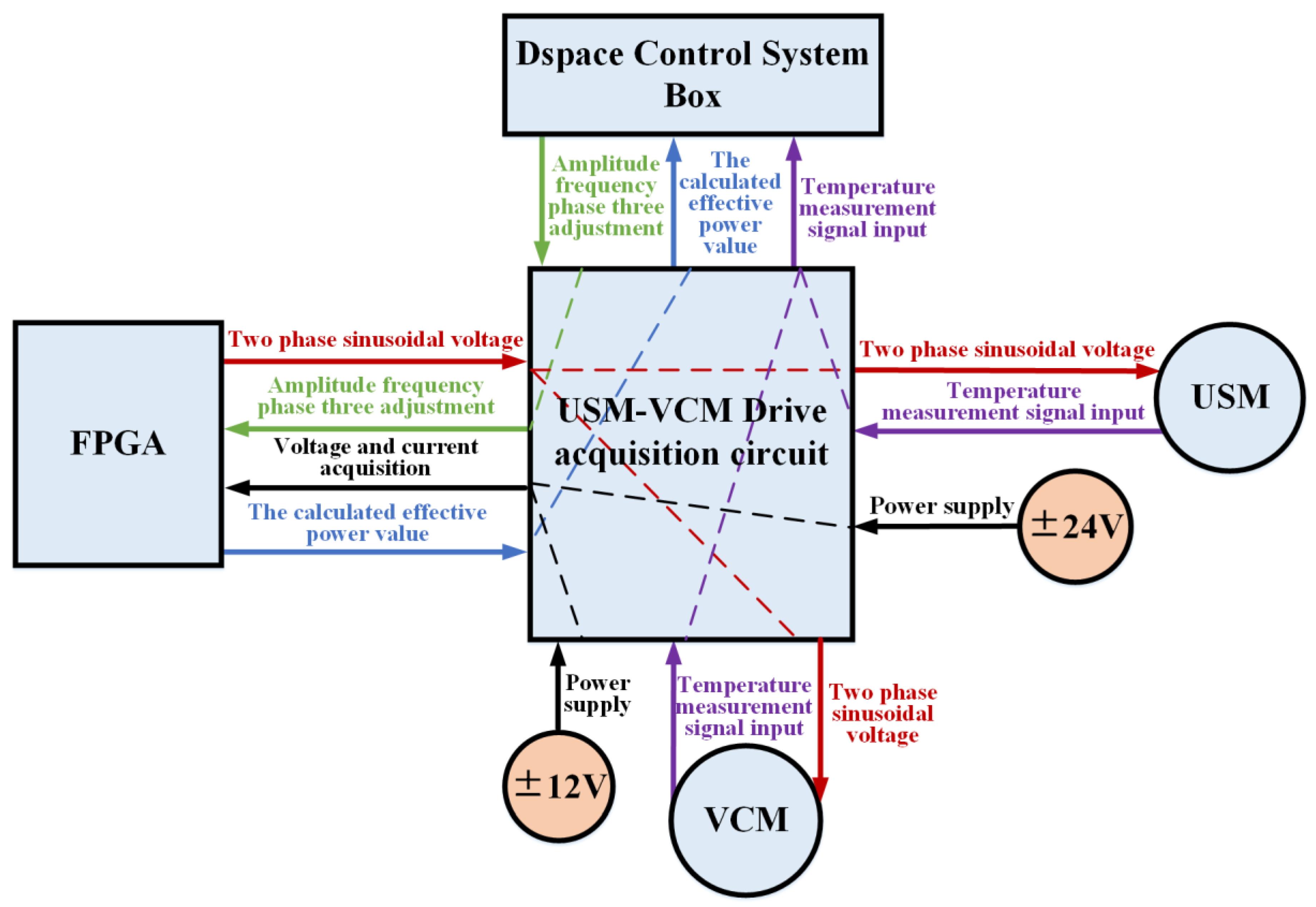
The multi-gimbal electro-optical pod is a complex system. In order to make a thorough analysis of the multi-gimbal electro-optical pod, the first step is to study the coarse–fine composite mechatronic system. Then, the whole system can be deeply analyzed. This is a research process, not a one-step process. According to the characteristics of the USM, VCM, dSPACE (control system box (developed by Germany dSPACE company, a software and hardware platform based on matlab control system development and semi-physical simulation), and FPGA (field programmable gate array), the circuit connection design is shown in Figure 1.
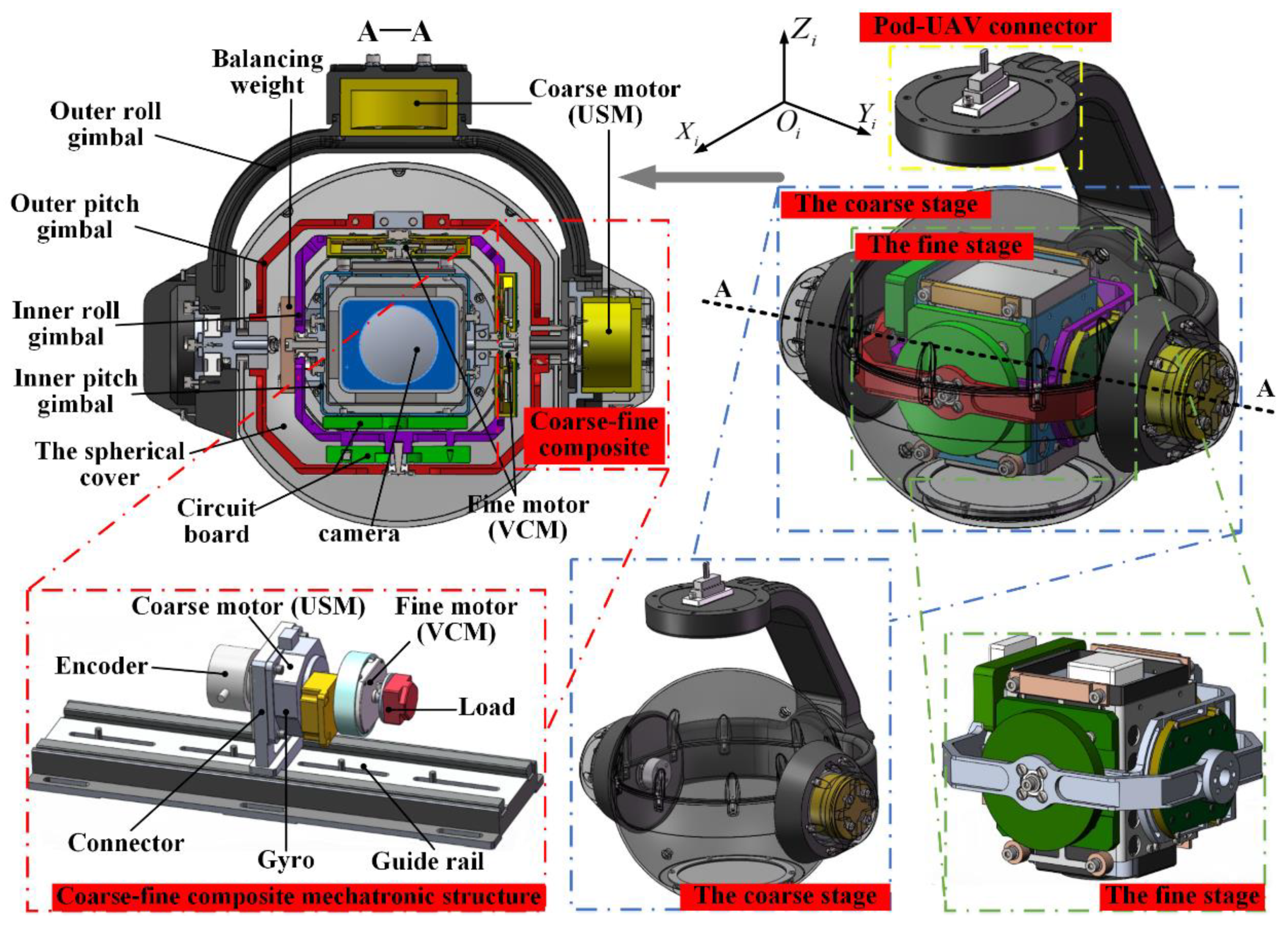
The coarse–fine composite mechatronic system of a UAV two-axis four-gimbal electro-optical pod is shown in Figure 2. The main objective of this manuscript is to design an ultralight electro-optical pod with a weight of less than 1 kg and miniaturization within .
The USM-VCM drive acquisition circuit connection design of a multi-gimbal electro-optical pod includes the following basic links:
- The dSPACE control system box outputs the three adjustment signals of the amplitude frequency phase, transformed by the drive acquisition circuit and received by the FPGA. The control signal occurs in the FPGA module and generates three two-phase parameters to adjust the sinusoidal wave.
- Two-phase sinusoidal voltage is generated by the drive acquisition circuit to generate the signal that meets the driving requirements of the USM and VCM, and then drives the coarse–fine dual stage motors for normal operation.
- Voltage-current detection is realized at the input end of the USM and VCM through voltage and current sensors. The detected voltage is input into the FPGA.
- The measured voltage-current amplitude and phase difference are calculated in the FPGA to obtain the effective power of the motor when it is working.
- The lead wire of the temperature sensor inside the USM and VCM is connected to the drive acquisition circuit, and the output voltage after amplification is regulated by the dSPACE control system box.
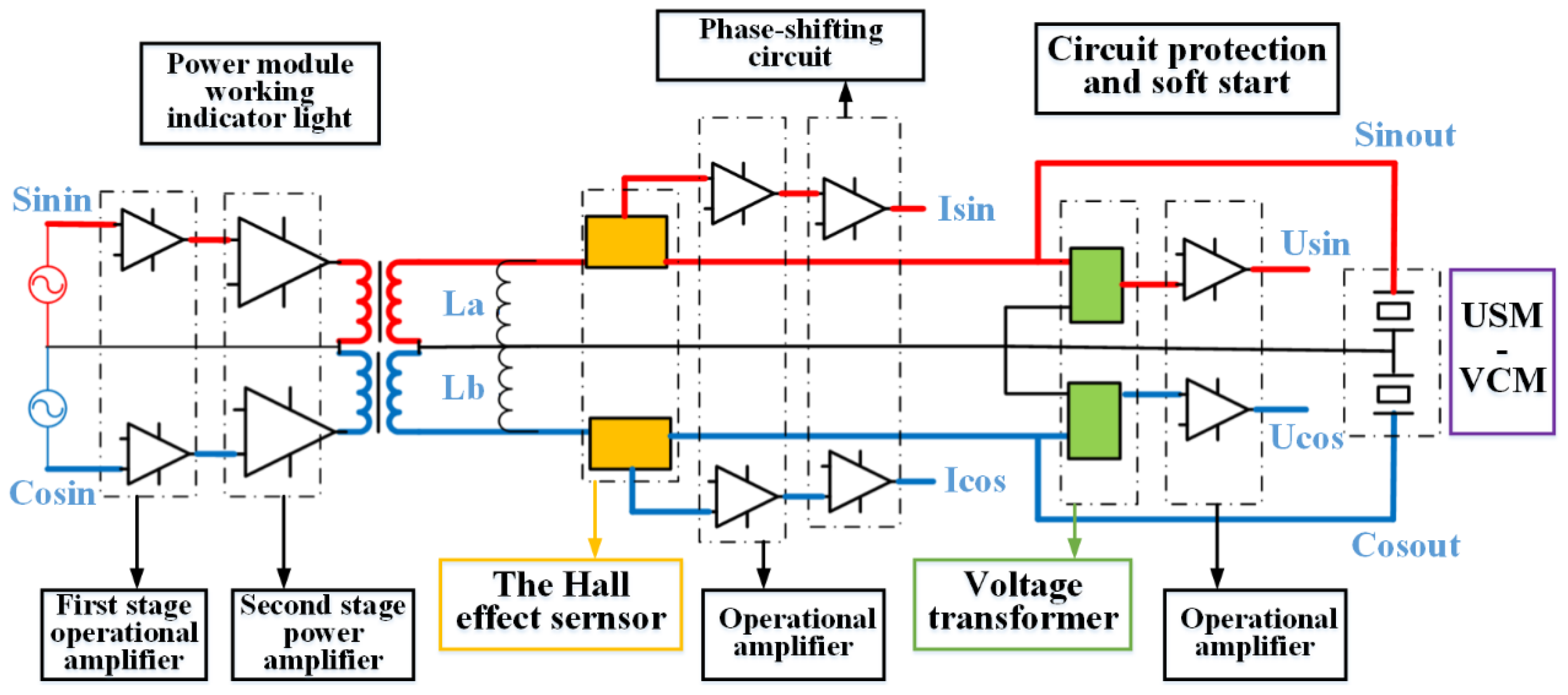
The main component of the USM-VCM coarse–fine composite drive acquisition circuit adopts the design idea of “first stage operational amplifier + second stage power amplifier + transformer + matching inductance”. The current detection component circuit adopts the design idea of “Hall effect sensor module + operational amplifier + advance phase amplifier”. The circuits of the driver and detection share the same ground line. The drive acquisition circuit is shown in the Figure 3.
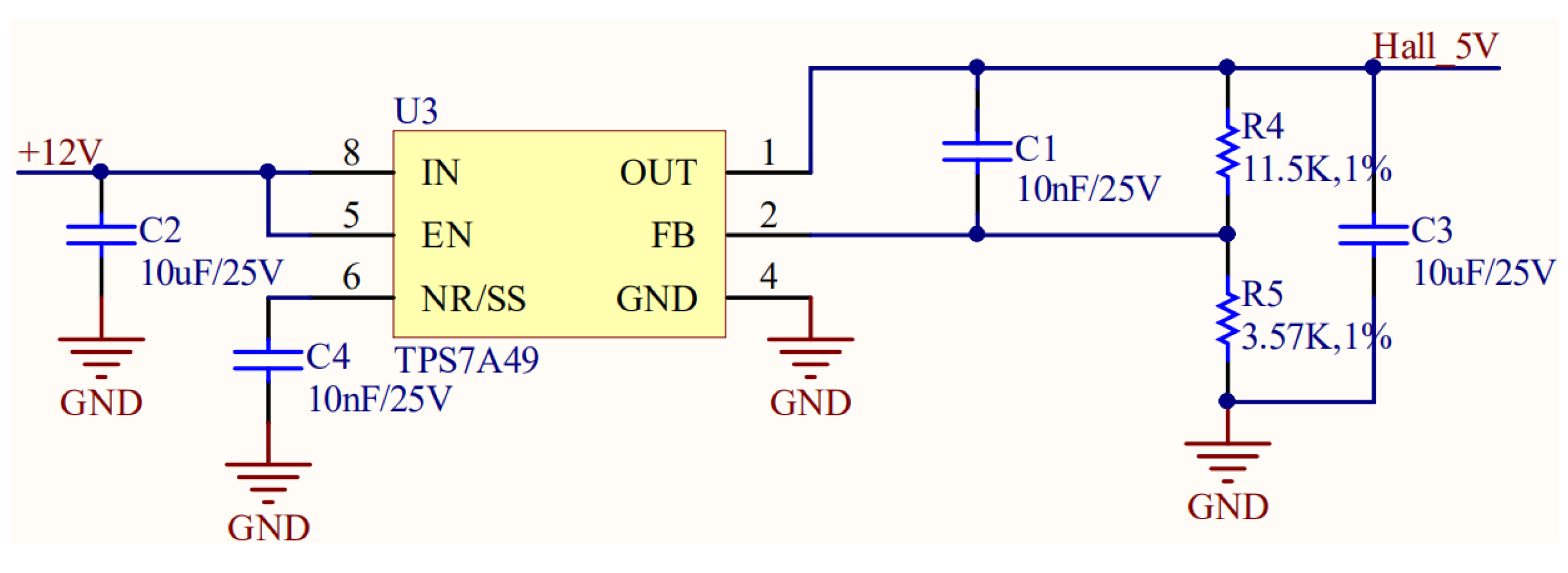
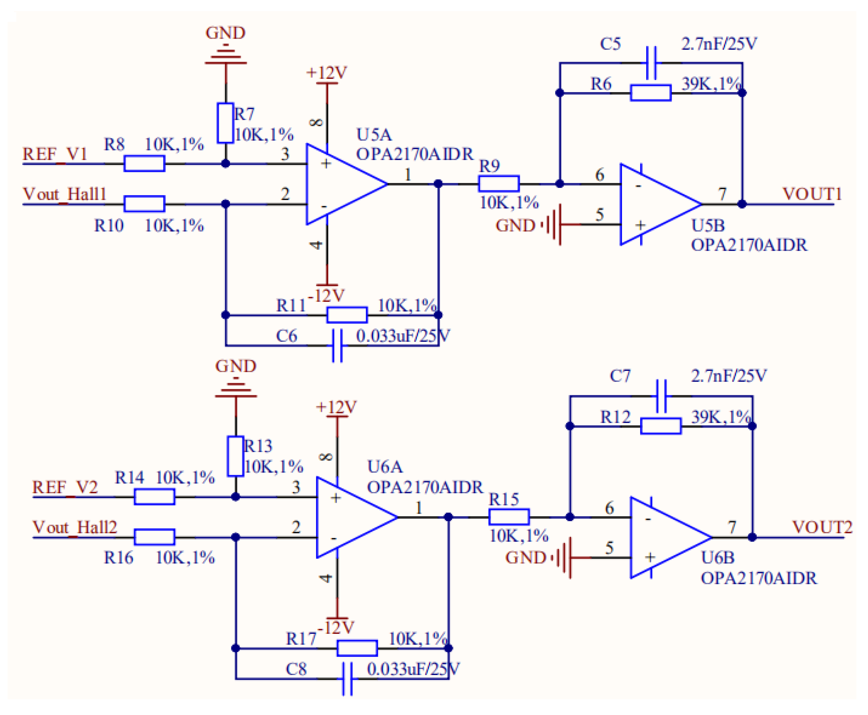
The interior of the VCM contains the Hall power supply circuit and the position signal conditioning circuit, as shown in Figure 4 and Figure 5. Debiasing, amplification, and filtering of position signals should be completed on the circuit board. The results will be directly output. Each device uses a smaller size package and the reference voltage used in the circuit calculation is adjustable.
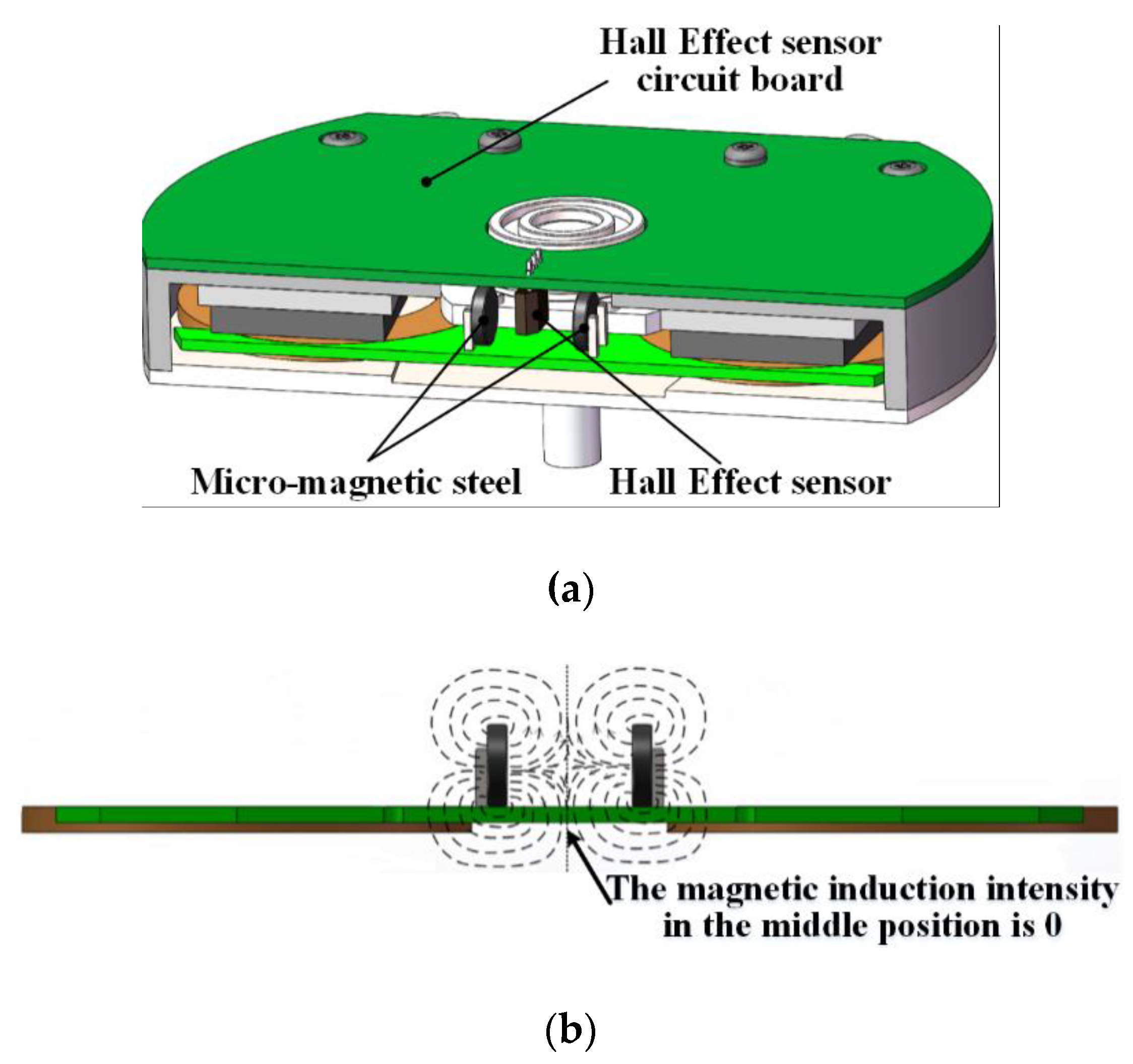
As shown in Figure 6, the two pieces of micro-magnetic steel are installed on the rotor of the motor corresponding to the pole, and the magnetic induction intensity in the middle position of the micro-magnetic steel is 0. When the output angle of the motor is 0° (the motor rotor is 180°), the Hall element is in the middle of the pieces of micro-magnetic steel. The magnetic induction intensity on the surface of the Hall element is 0 and the output voltage of the Hall effect sensor is a certain value. When the motor works at a limited angle, the rotor of the motor deflects and the two micro-magnetic steels will also deflect at an angle.
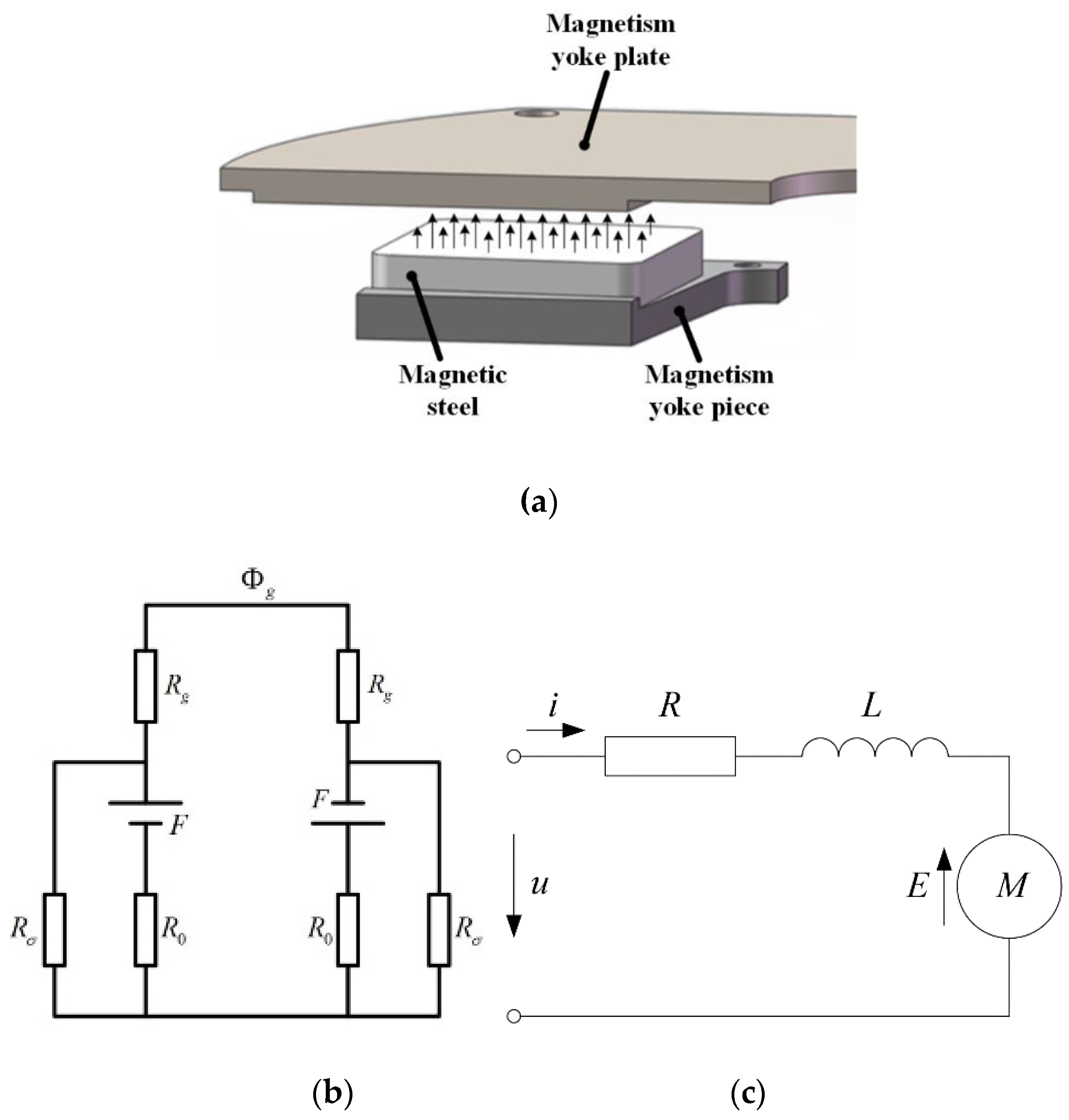
Magnetic circuits have similarities to electric circuits. Many physical quantities in magnetic circuits have corresponding physical quantities in electric circuits. Based on these similarities between magnetic and electric circuits, the method of similar circuit can be used for simulation and the equivalent magnetic circuit can be calculated. Figure 7a shows the structure model diagram of a single electromagnetic drive unit. The corresponding equivalent magnetic circuit is shown in Figure 7b.
Air gap reluctance, permanent magnet internal resistance, and permanent magnet magnetic potential are respectively:
where = air gap reluctance; = air gap thickness; = air permeability; = air gap area; = permanent magnet internal resistance; = magnetizing direction length of a single piece of magnetic steel; = relative permeability of permanent; = magnetizing area of the permanent magnet; = magnetic potential of the permanent magnet; = permanent magnet coercive force; = effective magnetic flux; = total magnetic flux; = y flux leakage quantity.
Because the permeability of soft iron is much higher than that of air, the magnetic resistance of soft iron is neglected in the magnetic circuit calculation. In addition, the magnetic resistance of the leakage magnetic circuit is treated as being equivalent in the calculation process. The magnetic flux leakage coefficient is taken as , and, by calculating the equivalent magnetic circuit, the derivation process of the air gap flux is as follows:
According to Figure 7c and Kirchhoff’s first law, two pieces of micro-magnetic were used as magnetic potential sources to obtain the magnetic flux leakage magnetic resistance. Then, this can be superimposed to obtain the air gap magnetic flux:
The air gap flux density can be obtained as:
Since an electromagnetic unit is composed of two copper wire coils, the motor contains two electromagnetic units. The Ampere force received by a single electromagnetic unit is:
where = Ampere force; = numbers of turns of copper wire coil; = gap flux density; = current flowing through the VCM; = length of the copper wire coil acting within the magnetic field. The output torque of the rotating voice coil motor is:
where = average lever arm length of VCM copper wire coil; is output constant of the VCM. The coil moves in a magnetic field under the action of an Ampere force, and an induced electromotive force is generated when the conductor cuts the magnetic field line. The direction of the induced electromotive force is obtained by Lenz’s theorem. The induced electromotive force is always opposite to the direction of the coil current. For the VCM, the reverse electromotive can be expressed as:
where = the reverse electromotive; = VCM speed; = VCM rotation angle. The dynamic voltage balance equation of coil loop can be obtained:
The output constant of the VCM is numerically equivalent to the reverse electromotive coefficient, . Therefore, the model of the rotating voice coil motor can be obtained:
For a N50 nd-fe-b sintered magnetic steel sheet with coerced force of Hc = 835 kA/m, the thickness of the permanent magnet is and the air gap thickness in the closed magnetic circuit is . The air gap area is equal to the blunt magnetic area of a single permanent magnet . Permeability in a vacuum is , and the relative permeability is . Thus:
Taking the flux leakage coefficient as , then:
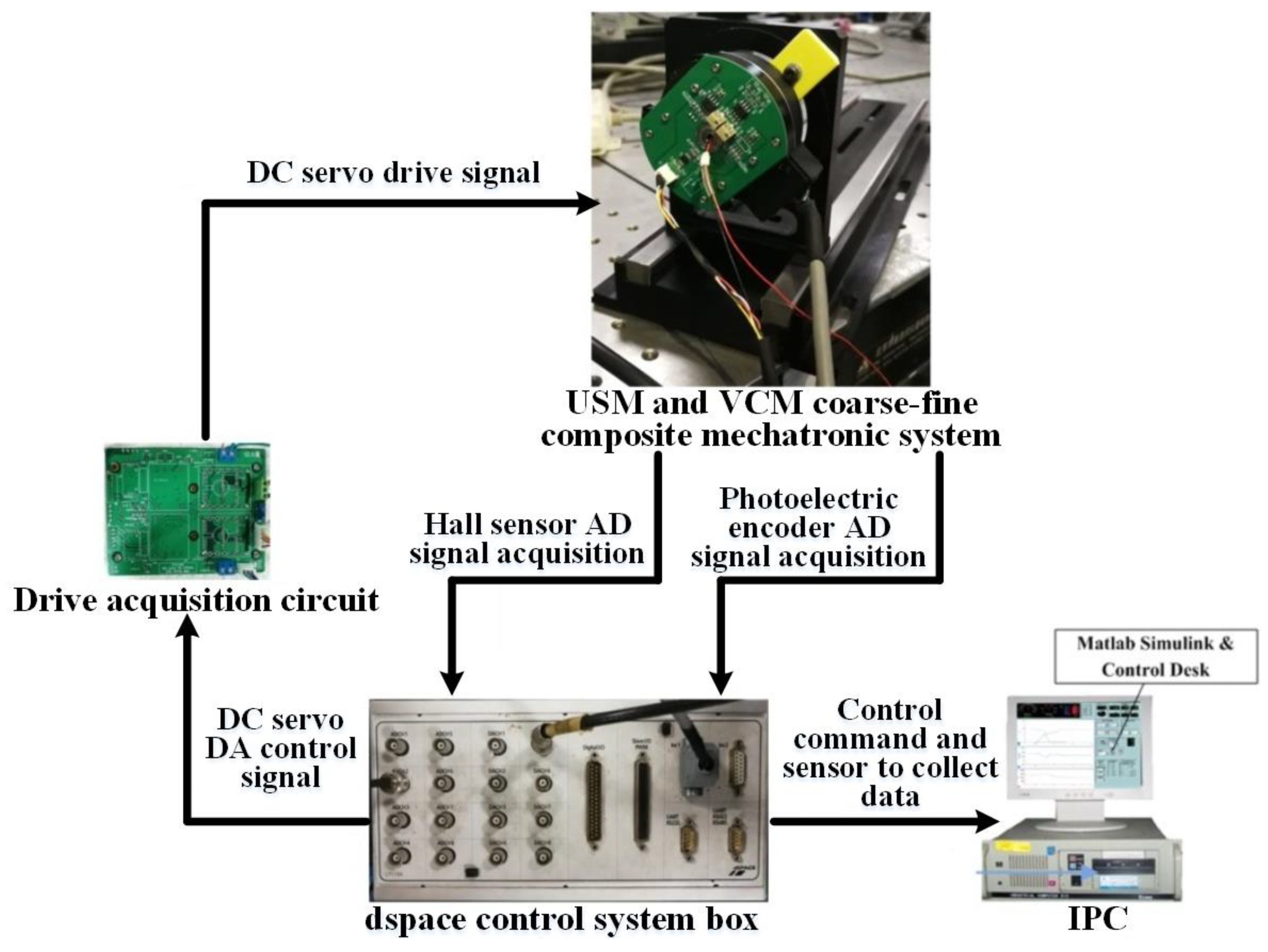
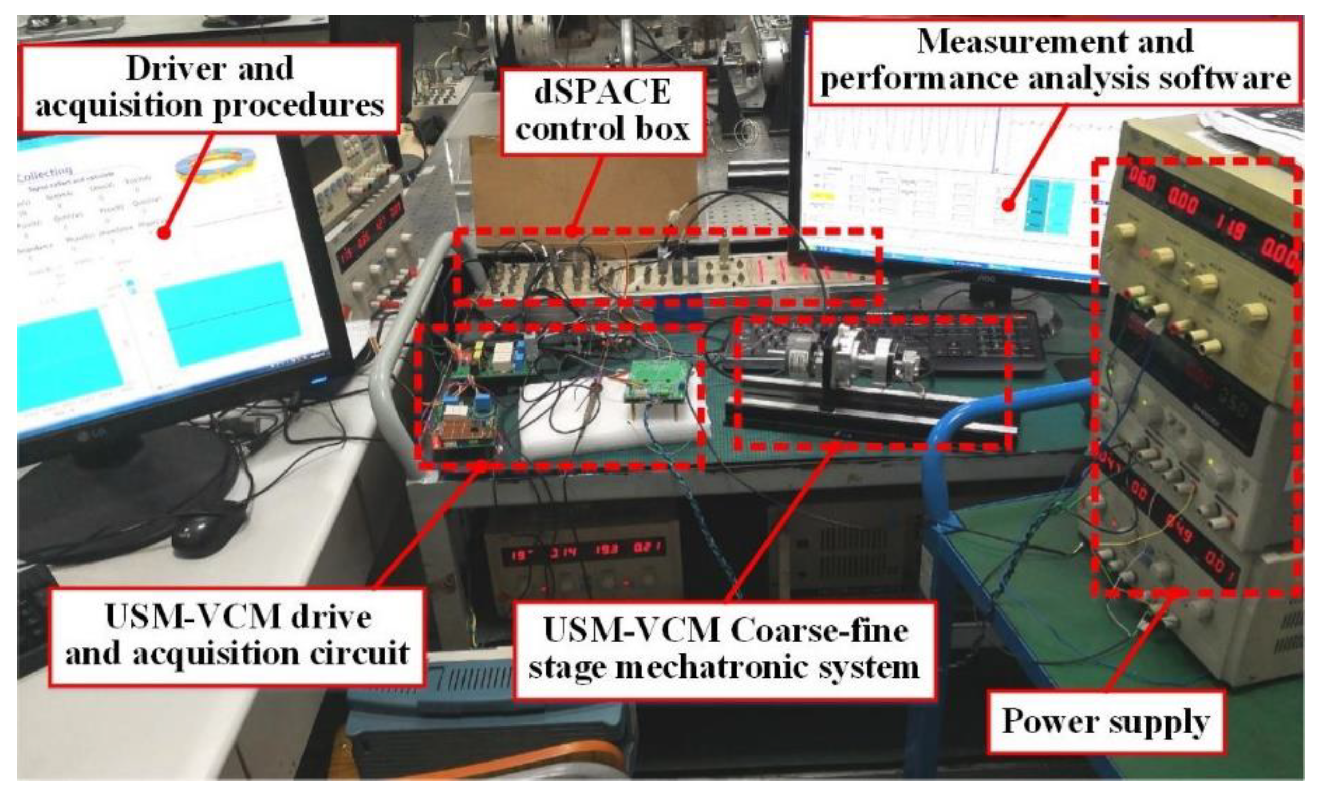
The main purpose of building the experimental platform as shown in Figure 8 was to test the performance parameters of the coarse–fine composite mechatronic system, understand its driving characteristics, and verify whether it meets the technical indicators.
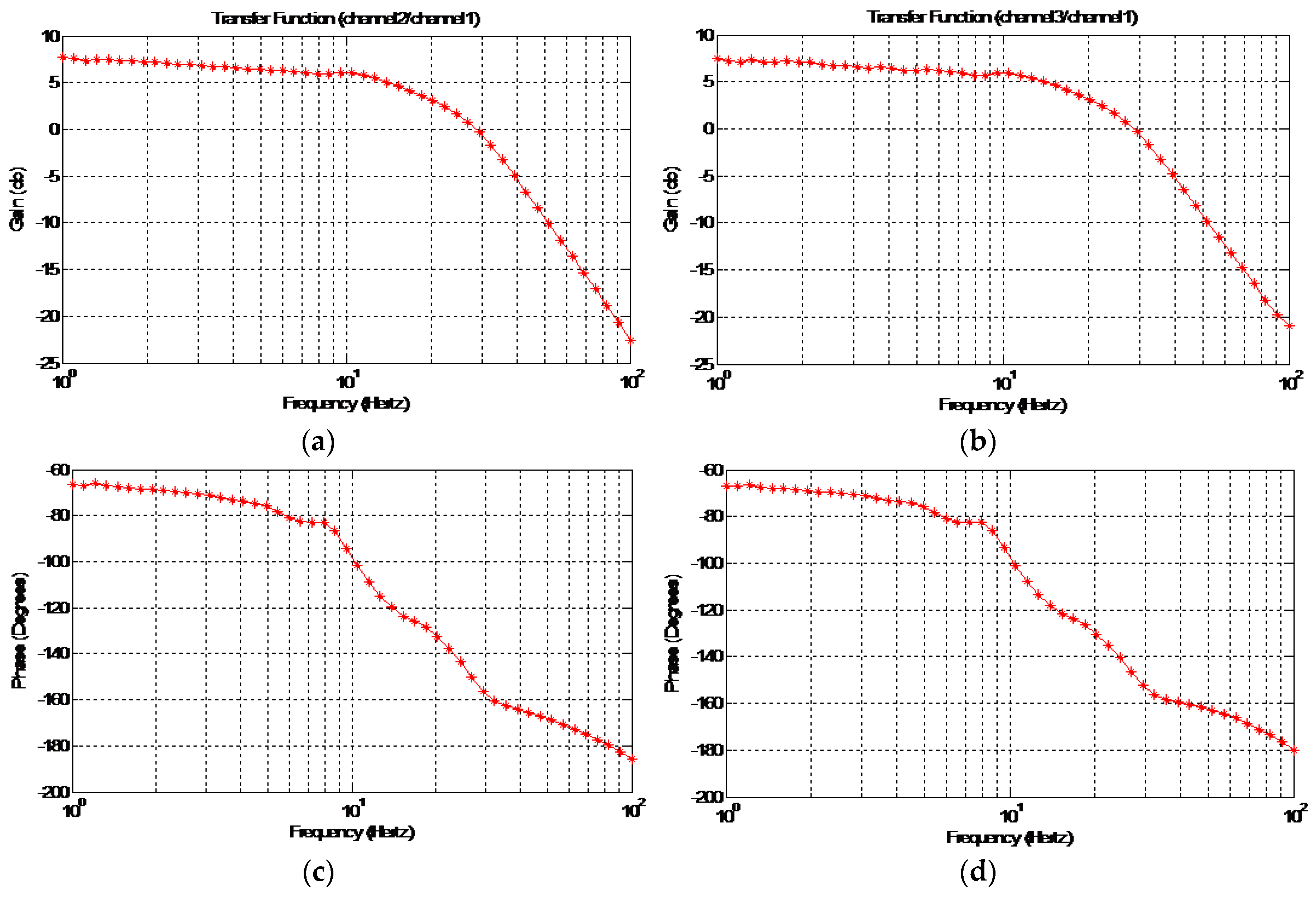
The position of the closed-loop was established based on the motor rotation angle calibration result and the sinusoidal frequency sweeping instruction was output through the dSPACE control system box to define the sweeping signal amplitude. The frequency range was 1–200 Hz. The position of the open- and closed-loop amplitude-frequency curve and phase-frequency curve of the VCM were obtained. Finally, the closed-loop bandwidth of the motor position was obtained.
In Figure 9a,c, the input signal of the system is the sinusoidal voltage instruction given, and the output signal of the system is the angle signal after Hall calibration. In Figure 9b,d, the input signal of the system is also the sinusoidal voltage signal, and the output signal of the system is the incremental encoder angle signal after zero calibration. As shown in Figure 9a,b, due to the slope change of the amplitude-frequency characteristic curve, it can be divided into two stages. In the first stage, the slope can be approximated as 0.3 in the range of 0–10 Hz; in the second stage, the slope can be approximated as 2.5 in the range of 10–100 Hz. Thus, when the frequency is equal to 10 Hz, the (10, 5.1) coordinate point can be regarded as the pole. The pole of the amplitude-frequency curve is related to the mechanical characteristics of the motor itself. In this manuscript, the slope change is related to the internal magnetic field strength of the VCM, magnet material, and copper wire winding. The measurement results on the Hall effect sensor are consistent with those of the incremental encoder through the comparison under open-loop control in Figure 9, which proves the accuracy of the Hall effect sensor.
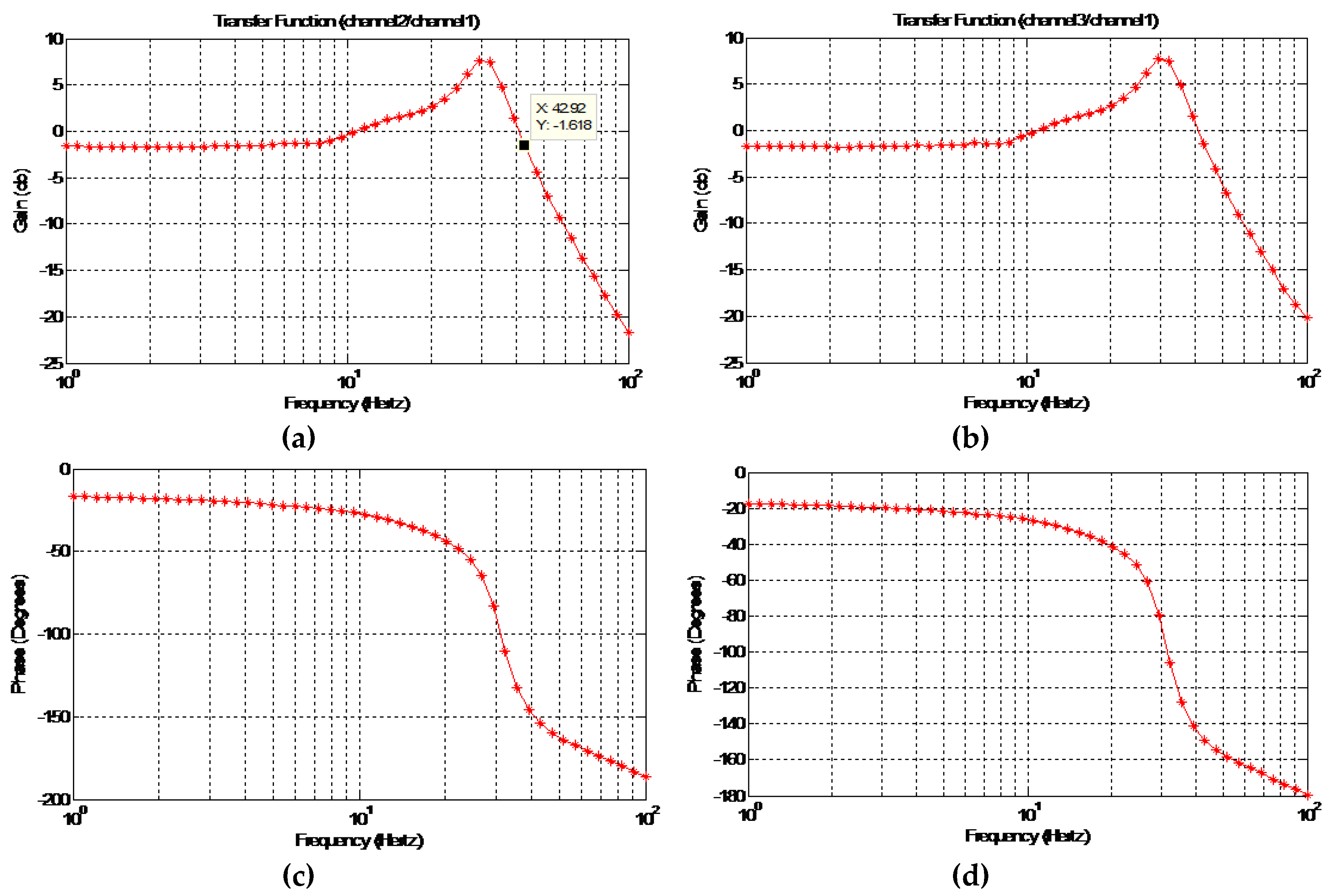
The closed loop of the angle position calibrated by the Hall effect sensor is used for the frequency sweeping identification. In Figure 10a–d, the information of the Hall effect sensor angle position and incremental encoder angle position was acquired at the same time. Bandwidth is defined as the frequency value when the closed-loop amplitude-frequency characteristic curve drops to −3 dB. Thus, as shown in the Figure 10a,b, when the gain is −3 dB, the frequency corresponding to the amplitude-frequency characteristic curve is approximately 40 Hz.
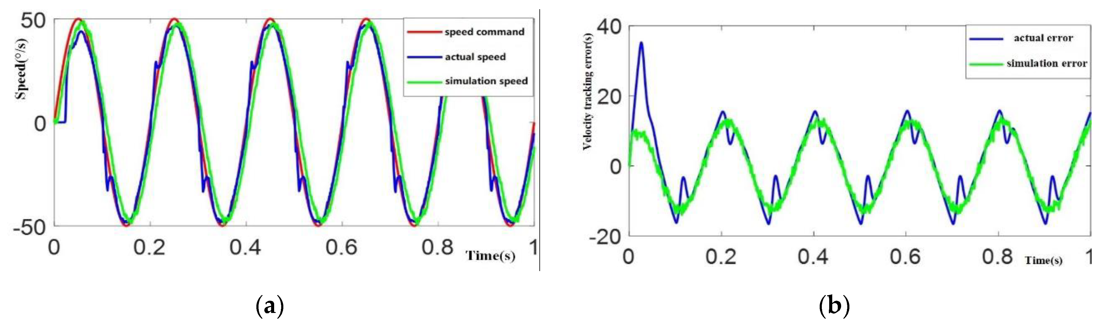
As shown in Figure 11a,b, two sinusoidal signals are designed to control the motor to obtain the characteristics of speed loop bandwidth and cut-off frequency. Figure 10a shows that the average value of the sinusoidal signal is 0, and the signal varies between −60°/s and 60°/s. Figure 11b shows the constant positive velocity with a bias value applied to the signal so that its average value is −60°/s and the sinusoidal amplitude value is 10. In Figure 11a,b, the red curve is speed command, the blue curve is actual speed and the green curve is simulation speed.
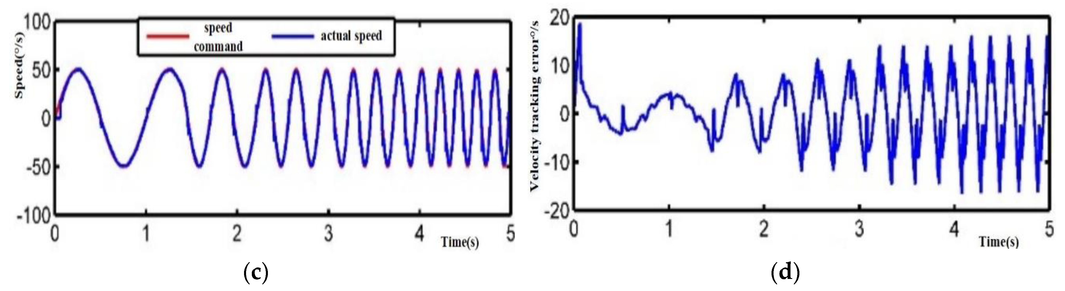
Figure 11c shows the USM disturbance suppression situation when the sinusoidal signal frequency gradually changes from 1 to 5 Hz, and Figure 11d shows the disturbance suppression situation when the frequency is 5 Hz. In Figure 11c,d, the blue curve is speed command and the blue curve is actual speed.
As shown in Figure 11, as the frequency increases, the error value of disturbance suppression also increases. Moreover, when the frequency is 5 Hz, the signal has a certain degree of distortion. The reason is that there is a dead zone for velocities greater than zero. It is found that if the frequency continues to increase, the actual speed signal will be seriously distorted. Thus, the speed loop bandwidth can be determined to be about 5 Hz.
When a sinusoidal bias signal is applied, the amplitude of the sinusoidal is 10. The frequency instruction increases from 0 to 25, with an interval of 5. After the speed closed-loop control of the USM, tracking remains accurate when the frequency of the instruction signal reaches 25 Hz. However, the tracking error increases with the increase of frequency. Thus, the bandwidth of the control system is not less than 25 Hz.
3. Euler Dynamics Model
As shown in Figure 2, the multi-gimbal electro-optical pod is a complex structure. In order to undertake thorough analysis and modeling of the two-axis four-gimbal electro-optical pod, the first step is to study the coarse–fine composite mechanical structure. Furthermore, based on the modeling of the coarse–fine composite mechatronic structure, modeling of the whole system can be analyzed.
In Figure 2, the working principle of the coarse-fine composite structure involves the definition of multiple coordinate systems, which are respectively explained as follows:
- Inertial coordinate system ({i}, ),
- UAV coordinate system ({d}, ),
- Coarse motor stator coordinate system ({u}, ),
- Coarse motor rotor coordinate system ({v}, ),
- Fine motor rotor coordinate system ({g}, ).
The coarse motor is fixedly connected with the guide rail through a threaded connection, without considering the damping effect between the structures.
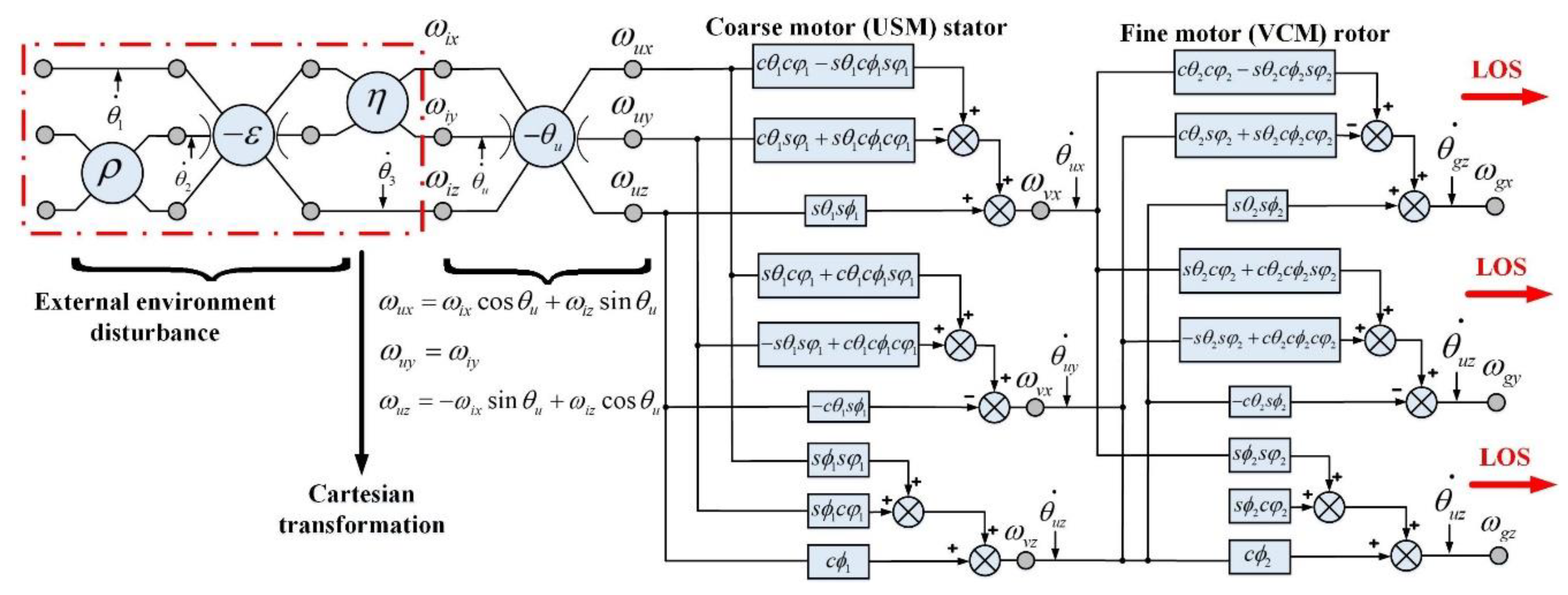
Due to the Euler transformation law of rigid body fixed point rotation [2], the kinematics coupling equations of the system {u} against system {i}, system {u} against system {v}, and system {v} against system {g} are:
The details of the dynamic parameter optimization equation derivation are already shown in reference [24]. The symbols used in the equation and Figure 12 are defined as follows: = the angular velocity vector of the coarse motor stator relative to the inertial coordinate system; = the angular velocity vector of the coarse motor rotor relative to the coarse motor stator coordinate system; = the angular velocity vector of the fine motor rotor relative to the coarse motor rotor coordinate system; = the angular velocity and its components on the coordinate axis; LOS = the line of sight; = the rotation transformation matrix; = Euler angles of rotation of each coordinate system.
Figure 12 shows the kinematics coupling relationship, which is abstracted from the parameters in the Euler rigid body dynamics expressed in Equations (17)–(19). The relationships of mechanical structure parameter optimization are divided into three stages: external environment disturbance, coarse motor (USM) stator, and fine motor (VCM) rotor. The final output is to maintain LOS (line of sight) stabilization. In Figure 12, the parameter relationships of each coordinate system can be directly analyzed and the parameters can be optimized in the controller, so as to achieve the goal of high precision control of the multi-gimbal electro-optical pod on the UAV. In order to simplify the analysis process of coarse-fine stage visual axis stabilization, this paper mainly discusses the conduction path and characteristics of UAV motion in relation to the coarse–fine composite mechanical structure. Therefore, the disturbance input of the external environment is analyzed as an inertial coordinate system, and the whole process of motion coupling of the coarse–fine mechatronic system is obtained through the transformation of the Cartesian coordinates along the system {u}, system {v}, and system {g}.
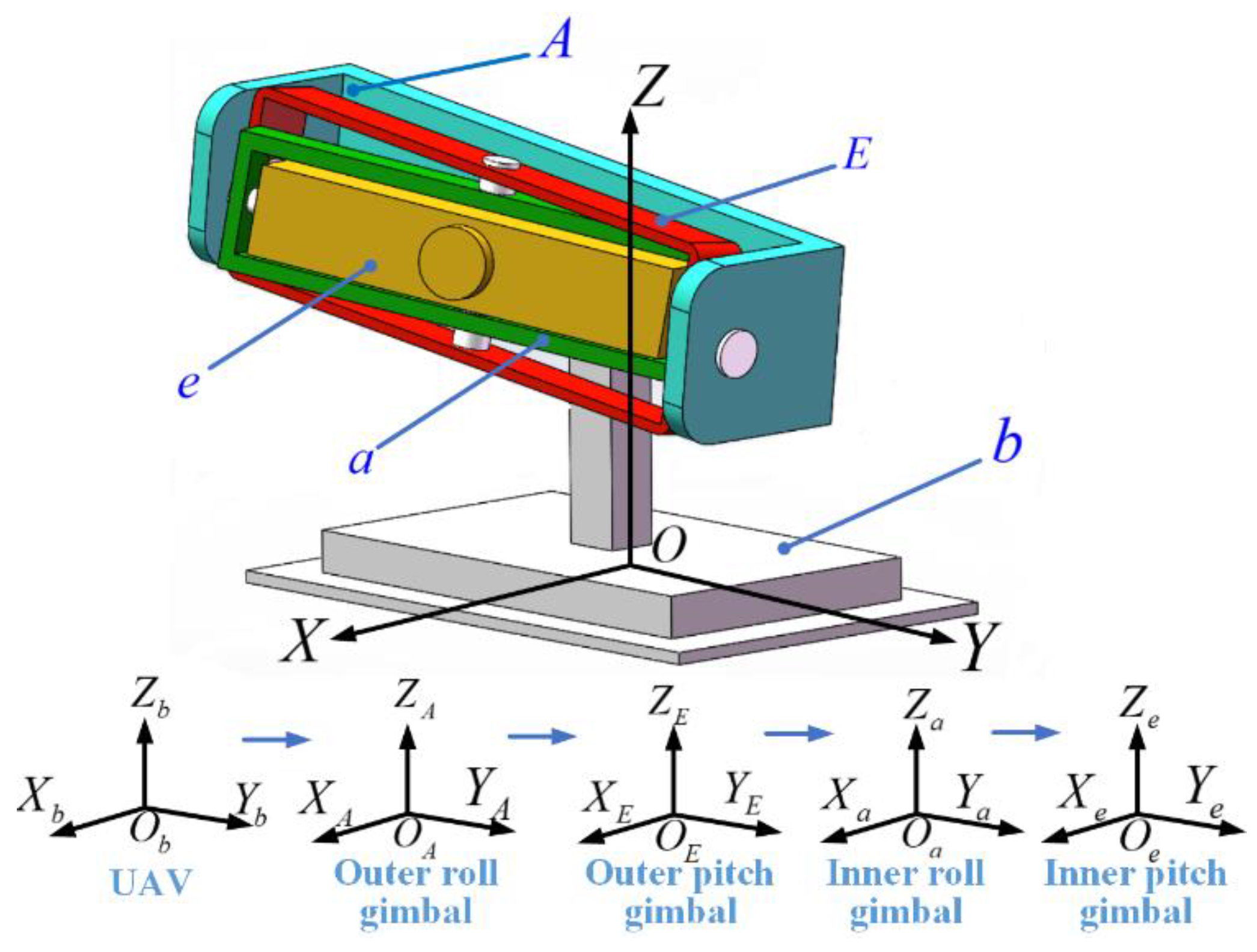
On the basis of the completion of the parameter optimization relationships of the coarse–fine composite mechanical structure, the two-axis four-gimbal electro-optical pod structure is modeled. The names of each gimbal coordinate system are defined in Figure 13.
The Cartesian coordinate system is simplified as follows:
- UAV coordinate system ({b}, ),
- Outer roll gimbal coordinate system ({A}, ),
- Outer pitch coordinate system ({E}, ),
- Inner roll gimbal coordinate system ({a}, ),
- Inner pitch gimbal coordinate system ({e}, ).
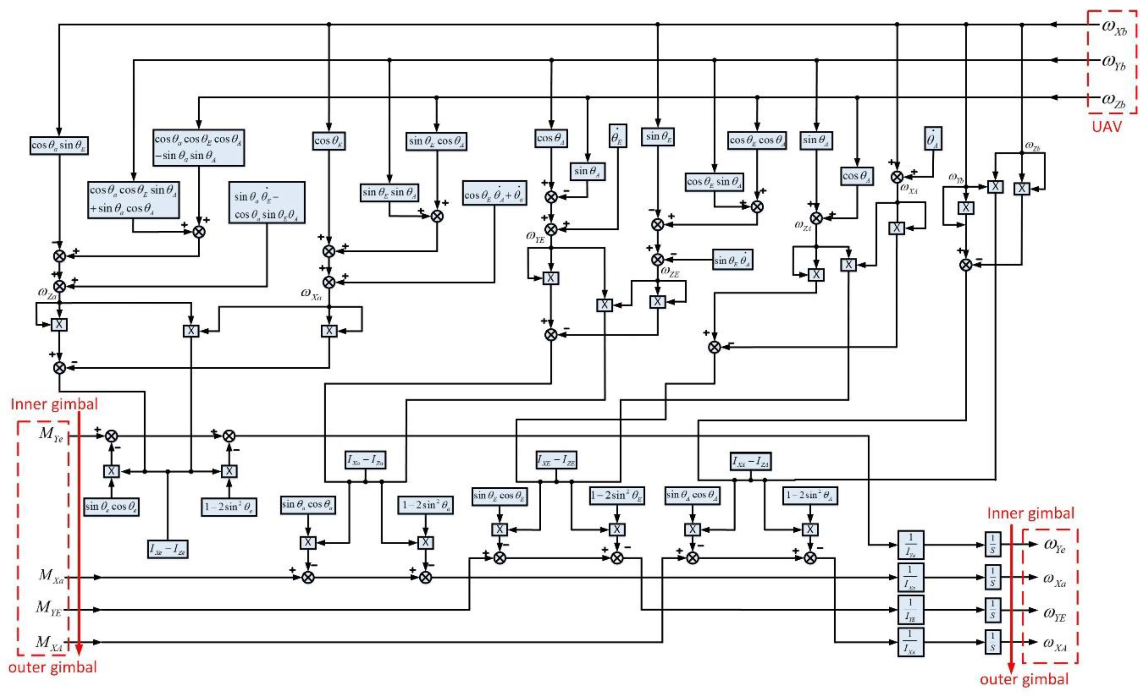
The motion between the gimbals of the two-axis four-gimbal structure produces a moment of inertia coupling. Assume the moment of inertia matrix of each gimbals is:
Then the coupling equations of moment of inertia of each gimbal rotating around its axis can be derived. The details of the derivation are shown in reference [24].
The symbols used in Figure 14 are defined as follows: = , , , represents the rotational inertia of the inner pitch, the inner roll, the outer pitch, and the outer roll of the gimbals along their respective rotation axis, = torque of the four gimbals relative to the rotation axis in the inertial coordinate system is the output torque of the motors, = angular velocity of inner pitch {e}, inner roll {a}, outer pitch {e}, outer roll {a} relative to inertial gimbal system {i}, = rotation angles of each gimbal.
In order to further study the parameter optimization mechanism of the two-axis four-gimbal structure, Figure 14 was drawn based on the Euler kinematics coupling of Equations (24)–(27) and Euler rigid body dynamics of Equations (17)–(19). In Figure 14, the torques caused by the kinematic parameters of the gimbals and the geometric coupling parameters are combined. The core problem is to enhance the disturbance suppression and ensure the high precision control of the LOS (line of sight) axis. The LOS (line of sight) axis is directly fixed to the inner pitch gimbal. Thus, it plays an important role in the stability of the LOS axis. According to reference [25], the derivation of the kinematic relationship equation can be obtained from the inner pitch gimbal mechanical equation:
For analysis and deduction of the moment of inertia coupling, from Equation (28) most of the interference moment is generated by the angular velocity of the forms through the moment of inertia subtraction. Therefore, the disturbing torque generated by the subtraction of rotational inertia is called inertia coupling torque. Then, the coupling moment of inertia received by the inner pitch gimbal is:
Methods to reduce the coupling torque of inertia are to minimize the rotation angle of the inner pitch axis, or reduce the difference between and . Thus, high precision control performance can be improved.
4. Coarse–Fine Composite Mechatronic Controller
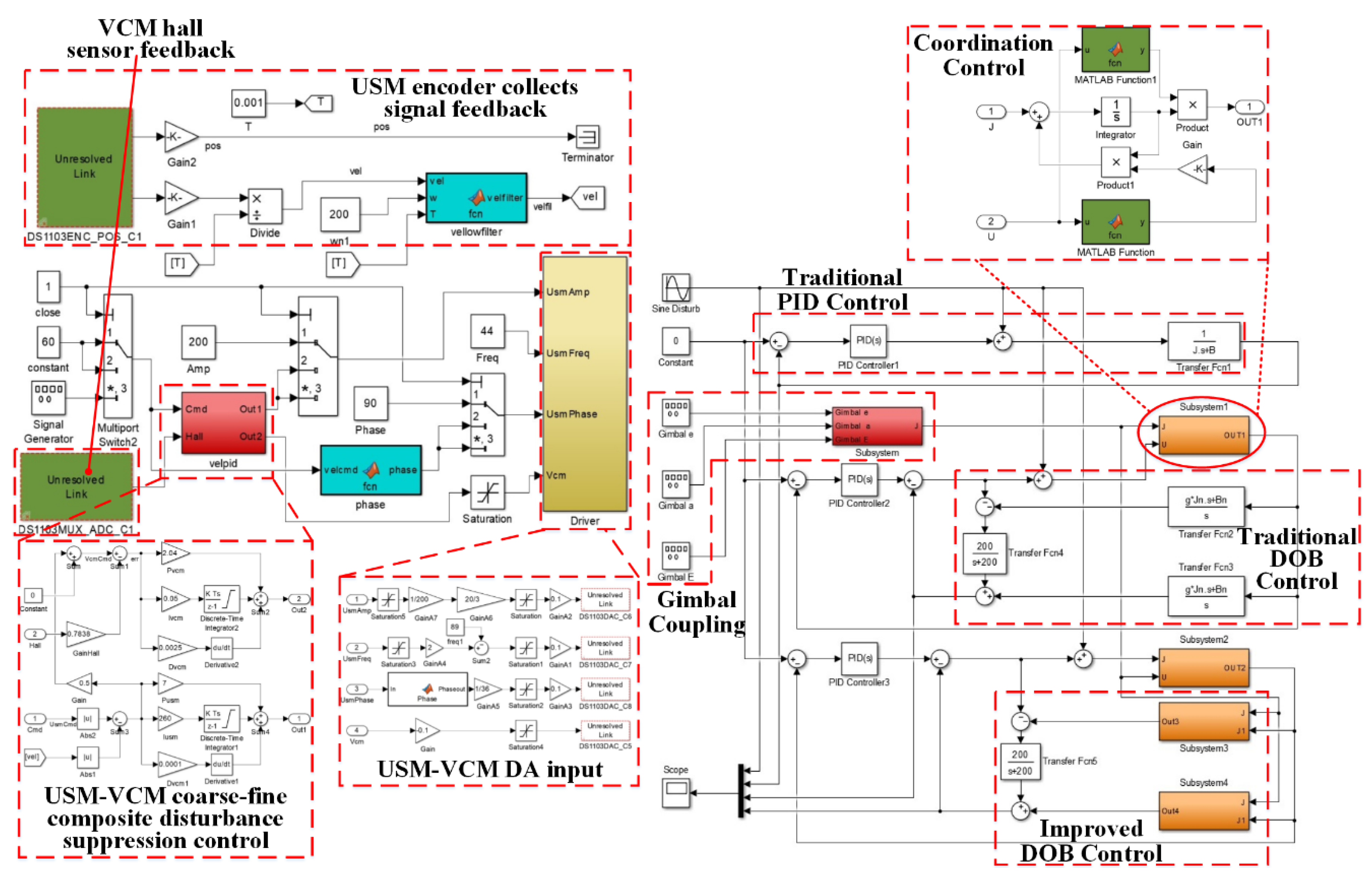
As shown in Figure 15, the purpose of this coarse-fine composite mechatronic controller is to prove the effectiveness of the mechatronic system design, the Euler dynamics model, and the USM-VCM drive acquisition circuit of the multi-gimbal electro-optical pod.
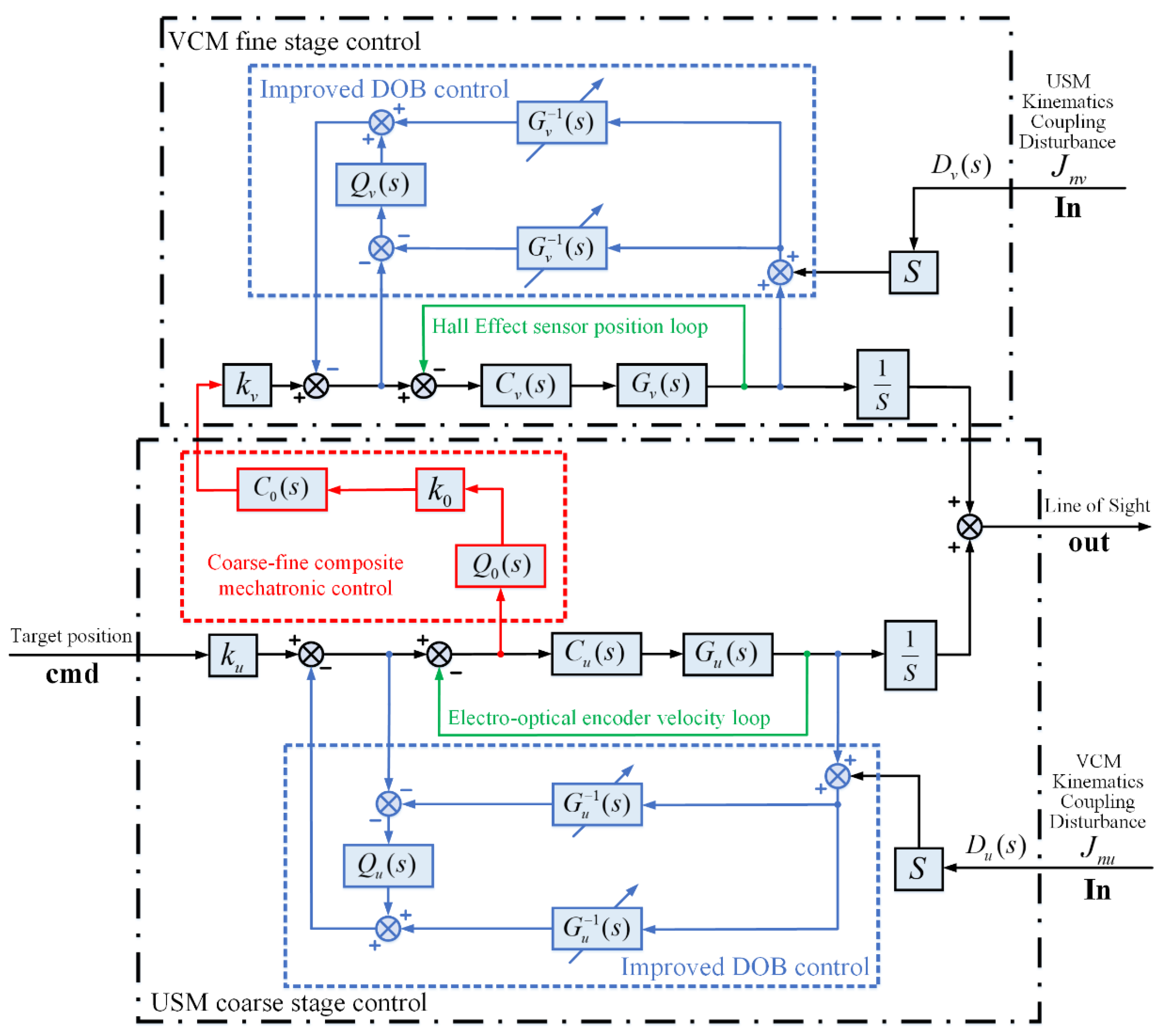
The symbols used in Figure 16 are defined as follows:
- = The loop controller of USM, VCM and macro-micro composite, respectively,
- = The control object of coarse–fine composite dual-stage motors,
- = The filter of the USM, VCM and macro-micro composite loop, respectively,
- = The kinematics coupling disturbance (submit Euler dynamic model),
- = The gain of USM, VCM, and coarse–fine composite loop.
In Figure 16, the coarse–fine composite mechatronic controller whole system consists of two sub-control loops. It is composed of a USM (ultrasonic motor) coarse-stage controller and VCM (voice coil motor) fine-stage controller. The whole system is input by a ‘cmd’ command signal (sinusoidal disturbance) and output by the rotation angle of LOS (line of sight). Furthermore, there are also two disturbance inputs derived after the Euler dynamics model that can monitor and compensate the kinematics coupling (moment of inertia coupling) of the two sub-control loops in real time.
In the improved DOB control loop, the control object is set as the coarse–fine composite mechatronic structure, and the minimum phase system under an ideal state is adopted [26,27,28]. The nominal inverse model of the control object is . Based on the kinematic coupling disturbance, which is derived by the Euler rigid dynamic model, the moments of inertia are substituted into the nominal inverse model of each stage control loop, thus realizing the real-time change of following the change of gimbal angle .
Because the control object is set as the coarse–fine composite mechatronic structure, and the minimum phase system under an ideal state is adopted, the nominal inverse model of the control object is .
Thus, the transfer function of the controlled object is:
We assume that the transfer function of the inverse model is:
In addition, we assume that the transfer function of the filter is:
From the Euler dynamics parameter optimization model, it is known that the coupling moment of inertia on the outer roll gimbal A of the electro-optical pod is:
As shown in Figure 16 and Figure 17, the USM coarse-stage sub-control loop is composed of a dual-level control loop. The first control loop is the inner loop, which is the electro-optical encoder velocity feedback loop. The second control loop is the outer loop, which is the improved DOB control loop.
The VCM fine-stage sub-control loop is also composed of the dual-level control loop. The first control loop is the inner loop, which is the Hall effect sensor position feedback loop. Moreover, the second control loop is the outer loop, which is the improved DOB control loop. The VCM’s improved DOB control loop is the same as the USM coarse-stage sub-control loop.
When the ‘cmd’ command signal is input, the dynamic model is automatically compiled into a kinematic coupling algorithm, and the kinematic coupling disturbance is input into two improved DOB control loops. Therefore, kinematic coupling disturbance can be changed in real time with the change of command signal, so as to achieve the purpose of real-time monitoring and compensation.
First, the ‘cmd’ command signal (sinusoidal disturbance) enters the feedforward loop of the USM coarse-stage control loop. Then, it passes through dual-level of compensation of the inner encoder velocity feedback loop and the outer improved DOB feedback loop. Furthermore, through the coarse–fine composite mechatronic control loop, the compensation error is substituted into the feedforward loop of the VCM fine-stage control loop as the input signal. Moreover, the compensated error and kinematic coupling disturbance are further compensated by the inner and outer dual-level controllers of the VCM fine-stage control loop. Finally, the actual rotation angle signal of the LOS is output, and the electro-optical pod then points to the tracking position. Stability of the coarse–fine composite mechatronic control is thus realized.
Table 1 shows the parameter settings and the performance of the experiment results, which is defined as:
- = USM coarse stage controller disturbance suppression output and VCM fine stage controller disturbance suppression output,
- = Sinusoidal wave disturbance and the deviation (compensate error) between the USM coarse stage controller disturbance suppression output,
- = Disturbance estimated deviation,
- , , = The PID control parameters.
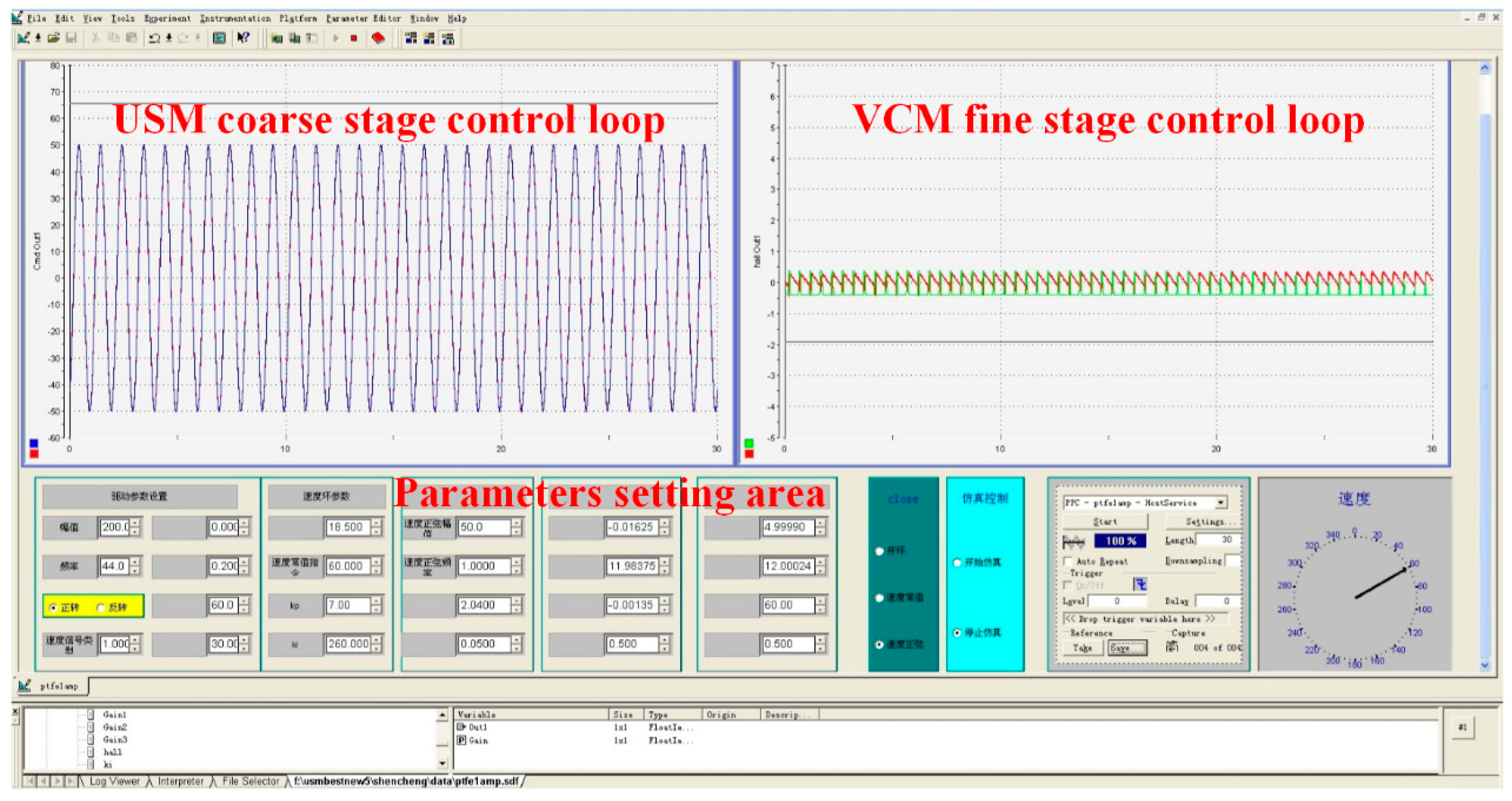
Figure 18 shows the experiment control desk operating interface. Firstly, the parameters of the traditional PID controller are set as: , and the value of the moments of inertia are set as from simulation. The parameters of the disturbance observer and its low-pass filter are set as: .
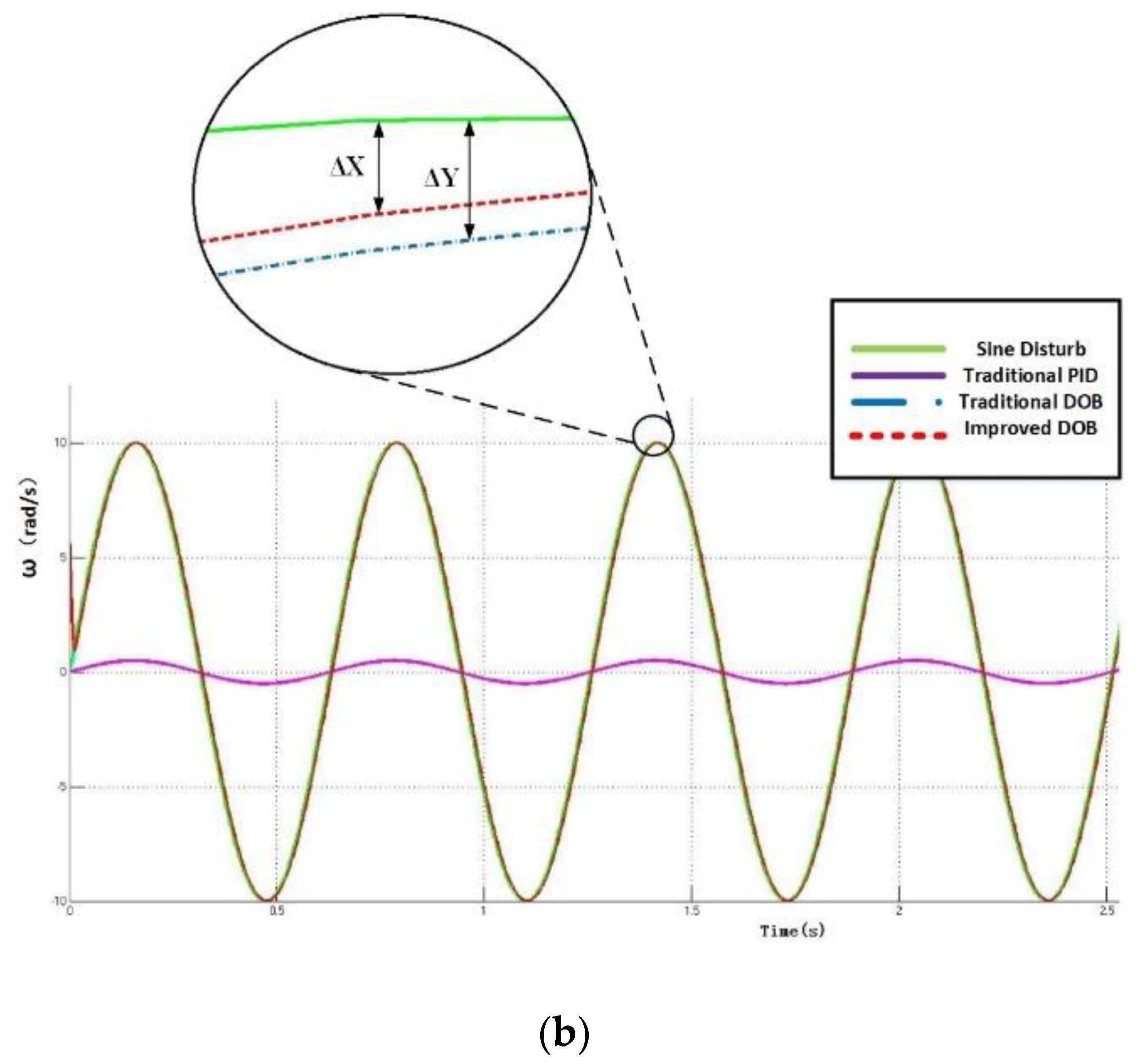
The parameters of USM-VCM coarse–fine composite mechatronic control loop are set as: coarse stage , fine stage . The coarse-stage disturbance signal of the USM adopts the sinusoidal wave input and the amplitude of the velocity sine is set as 28, the frequency of the velocity sine is 1, and the constant instruction of the velocity is 60.
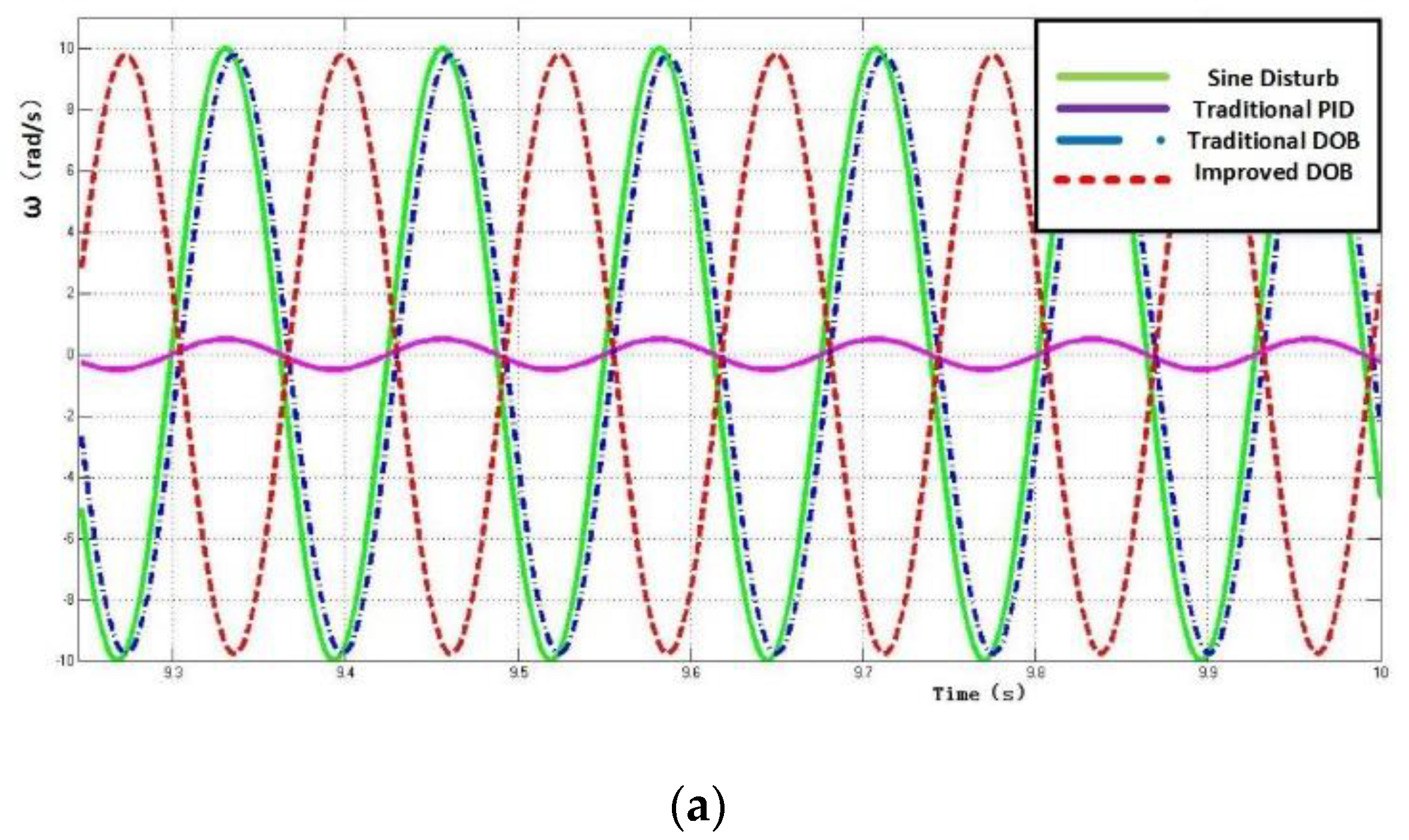
As shown in Figure 19a, there are four curves: sinusoidal wave disturbance, PID (proportion integration differentiation) method, traditional DOB method, and Euler dynamics parameters optimization DOB method.
As shown in Equation (35) and Figure 19b, the stability of the controller can be proved by comparing the deviation values of the three curves following the sinusoidal disturbance. It can be seen that the disturbance suppression effect of modeling using the improved DOB method is about 90% higher than the PID method. The experiment performance results are summarized in Table 1.
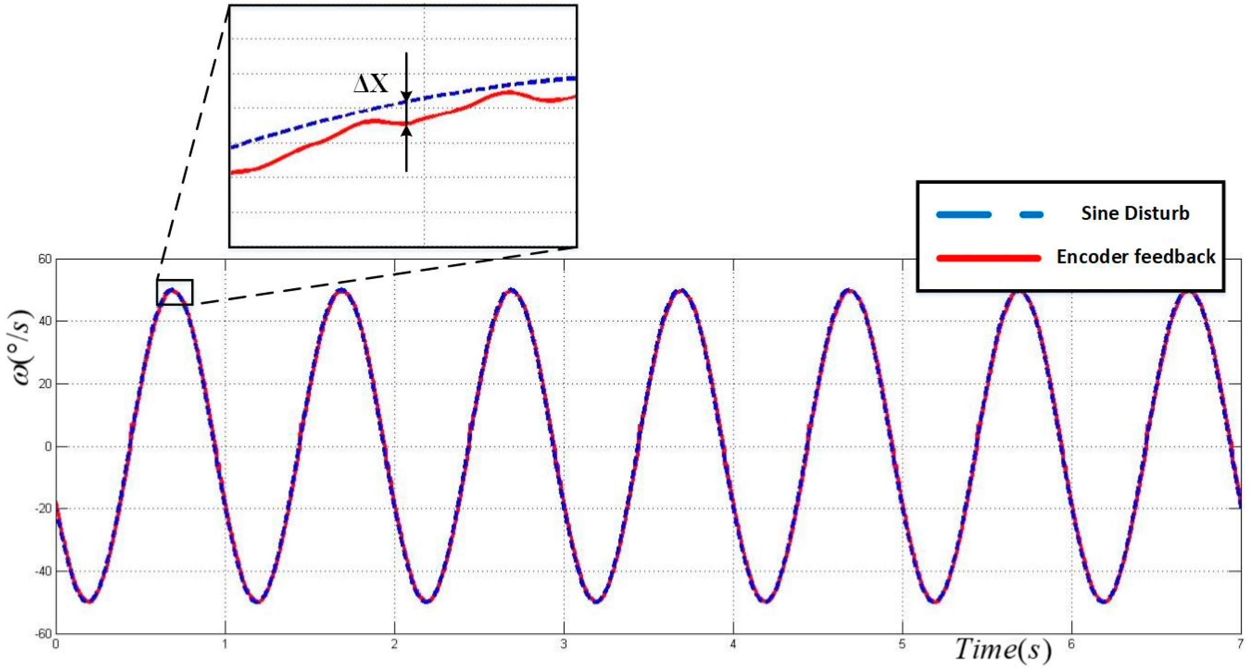
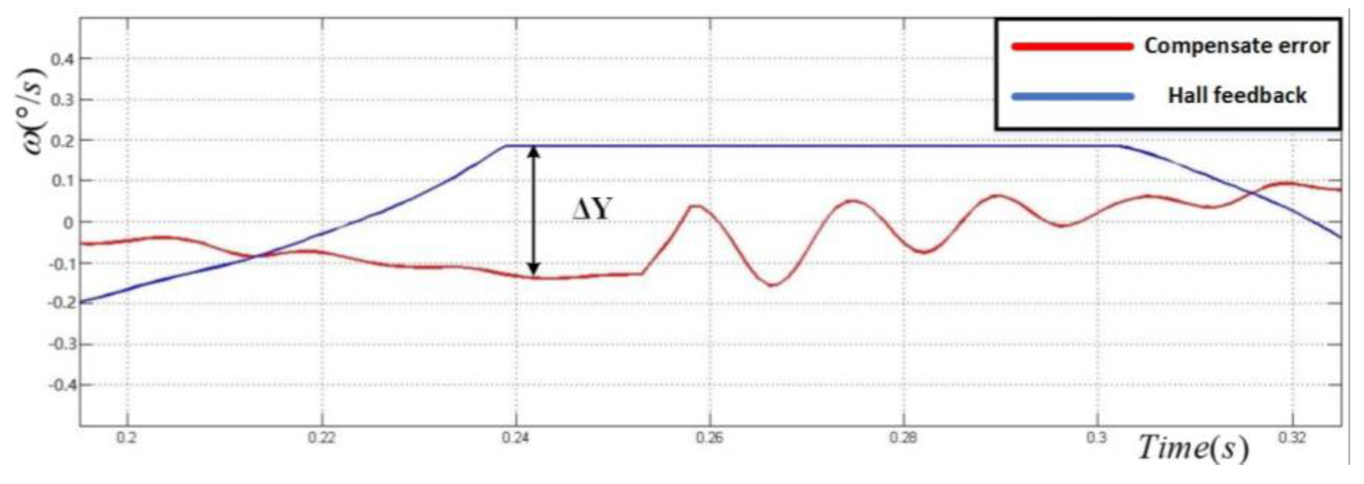
Figure 20 shows the USM controller encoder feedback curve and the sinusoidal disturbance curve. Figure 21 shows the VCM controller Hall effect sensor feedback curve and the deviation curve (compensated error) between the USM controller encoder feedback curve and the sinusoidal disturbance curve. The stability of the parameters optimization controller can be proved by comparing the deviation values of the two curves following the sinusoidal disturbance.
It can be seen from Equation (36) and Figure 21 that the disturbance suppression effect of the VCM controller can be improved by up to 90% on the basis of the USM controller.
It can be seen from Figure 22a that the estimated deviation is , and from Figure 22b that the estimated deviation is . Thus, the disturbance suppression impact of the DOB method with Euler dynamics modeling and the coarse–fine composite mechanical system is increased by up to 90% compared to the PID method and is 20% better than the traditional DOB method. The experiment performance results are summarized in Table 1. Result shows the effectiveness of the coarse–fine composite mechatronic system, the USM-VCM drive acquisition circuit, and the Euler dynamics modeling.
5. Conclusions
This paper makes an in-depth study of the modeling and stability analysis of a coarse–fine composite mechatronic system in a UAV multi-gimbal electro-optical pod. The conclusions are as follows:
- The core goal of this manuscript is to address the issue of coarse–fine composite mechatronic system stability of a UAV multi-gimbal electro-optical pod using USM-VCM mechatronic design, Euler dynamics modeling, and stability DOB control. In response to this problem, a Hall effect electromagnetic circuit and USM-VCM drive acquisition circuit are designed. An aerospace USM is used as the coarse-stage, and an ultralight VCM with high positioning precision is designed as the fine-stage. The Hall effect sensor and micro-magnetic steel are tested to design the VCM as the fine-stage. The VCM designed in the present work has positioning precision of only 8.7 μrad, bandwidth of 40 Hz, and mass of less than 70 g. According to the effectiveness verification of the VCM magnetic circuit, the theoretical formulae of the air gap magnetic induction intensity and motor output torque are obtained.
- Secondly, the Euler rigid body dynamics model of the coarse–fine composite mechanical system and the two-axis four-gimbal mechanical structure are obtained. The kinematics coupling compensation matrix and mechanical parameter optimization method between the gimbals are derived. The Euler dynamics equation in the Cartesian coordinate system is derived to solve the pre-selection and check problem of the coarse–fine composite mechatronic system.
- Thirdly, the model is substituted into the DOB suppression control, which can monitor and compensate the motion coupling between the coarse–fine composite mechatronic systems in real time. Results show that the disturbance suppression impact of the DOB method with the Euler optimization model and USM-VCM mechatronic design is increased by up to 90% compared to PID and is 20% better than the traditional DOB method.
- Finally, this manuscript is based on the coarse–fine composite mechatronic system design of the multi-gimbal UAV electro-optical pod. This manuscript is valuable for all researchers interested in USM-VCM coarse–fine composite mechatronic system modeling, mechatronic drive acquisition circuits, and multi-gimbal electro-optical applications.
Author Contributions
C.S. designed the parameters optimization method and controller and carried out experimental research on the effect of the modeling and algorithm. D.F. and S.F. guided the research and proposed the ideas and revisions of the paper. N.C. provide help with control and simulation. R.T. provide structure model. C.S. and S.F. revised the paper. All authors have read and agreed to the published version of the manuscript.
Funding
This research received no external funding.
Acknowledgments
The author would like to thank all the teachers and colleagues who provided inspirations and equipment in the experiment. The author would like to thank all the anonymous reviewers for their meticulous comments and helpful suggestions.
Conflicts of Interest
The authors declare no conflict of interest.
Nomenclature
| UAV | (unmanned aerial vehicle) |
| USM | (ultrasonic motor) |
| VCM | (voice coil motor) |
| DOB | (disturbance observer) |
| PID | (proportion integration differentiation method) |
| FPGA | (field programmable gate array) |
| DA | (digital-to-analogue) |
| AD | (analogue-to-digital) |
| LOS | (line of sight) |
| dSPACE | (control system box (developed by Germany dSPACE company, a software and hardware platform based on matlab control system development and semi-physical simulation) |
| PDPC | (process decision program chart) |
References
- Da-Peng, F.; Zhi-Yong, Z.; Shi-Xun, F.; Yan, L.I. Research of the basic principles of E-O stabilization and stabilization and tracking devices. Opt. Precis. Eng. 2006, 14, 673–680. [Google Scholar]
- Rue, A.K. Precision Stabilization Systems. IEEE Trans. Aerosp. Electron. Syst. 1974. [Google Scholar] [CrossRef]
- Rue, A.K. Stabilization of precision electro-optical pointing and tracking systems. IEEE Trans. Aerosp. Electron. Syst. 1969, 5, 805–819. [Google Scholar] [CrossRef]
- Rue, A.K. Calibration of Precision Gimbaled Pointing Systems. IEEE Trans. Aerosp. Electron. Syst. 1970, 5, 697–706. [Google Scholar] [CrossRef]
- Rue, A.K. Correction to Stabilization of precision electro-optical pointing and tracking systems. IEEE Trans. Aerosp. Electron. Syst. 1970, 6, 855–857. [Google Scholar]
- Rue, A.K. Confidence Limits for the Pointing Error of Gimbaled Sensors. IEEE Trans. Aerosp. Electron. Syst. 1966, 6, 648–654. [Google Scholar]
- Royalty, J. Development of Kinematics for Gimballed Mirror and Prism Systems. SPIE 1990, 1304, 262–274. [Google Scholar]
- Kennedy, P.J.; Kennedy, R.L. Direct versus Indirect Line of Sight (LOS) Stabilization. IEEE Trans. Control Syst. Technol. 2003, 11, 3–15. [Google Scholar] [CrossRef]
- Masten, M.K.; Sebesta, H.R. Line-of-Sight Stabilization/Tracking System: An Overview. In Proceedings of the American Control Conference, Minneapolis, MN, USA, 10–12 June 1987; pp. 1477–1482. [Google Scholar]
- Bao, W.L.; Huang, X.L.; Lu, X.L. Dynamic modeling and coupling analysis of a multi-gimbal electro-optical platform. J. Harbin Eng. Univ. 2009, 30, 893–897. [Google Scholar]
- Cheng, Y.; Liu, Y.; Wang, M.S.; Ai, W.J. Dynamic modeling and coupling analysis of two-axis four-gimbal stabilized platform. Autom. Instrum. 2016, 195, 195–197. [Google Scholar]
- Kong, D.J.; Dai, M.; Yu, X. Movement Coupling Analysis of Airborne Electro-Optical Platform with Two Axis Four Framework. J. Chang. Univ. Sci. Technol. 2013, 6, 24–27. [Google Scholar]
- Wei, Z.; Ke, S.; Li, Y.B. Coarse-to-Fine UAV Target Tracking With Deep Reinforcement Learning. IEEE Trans. Autom. Sci. Eng. 2018, 16, 1545–1554. [Google Scholar]
- Wang, F.J.; Huo, Z.C.; Liang, C.M.; Shi, B.C.; Tian, Y.L.; Zhao, X.Y.; Zhang, D.W. A Novel Actuator-Internal Micro/Nano Positioning Stage with an Arch-Shape Bridge Type Amplifier. IEEE Trans. Ind. Electron. 2019, 66, 278–288. [Google Scholar] [CrossRef] [Green Version]
- Qian, J.B.; Bao, L.P.; Yang, X.J.; Ji, C.K. Modeling and Identification of Vibration Transmission in a Dual-Servo Stage. J. Sound Vib. 2018, 432, 249–258. [Google Scholar] [CrossRef]
- Choi, Y.M.; Gweon, D.G. A High-Precision Dual-Servo Stage Using Halbach Linear Active Magnetic Bearings. IEEE/ASME Trans. Mechatron. 2011, 16, 925–931. [Google Scholar] [CrossRef]
- Jia, J.H.; Song, J.P. Coupling Disturbance of Two-axis Stabilization Platform Based on Lagrangian Modeling. J. Mil. Transp. Univ. 2016, 18, 91–95. [Google Scholar]
- Boettcher, U.; Raeymaekers, B.; Callafon, R.A.; Talke, F.E. Dynamic Modeling and Control of a Piezo-Electric Dual-Stage Tape Servo Actuator. IEEE Trans. Magn. 2009, 45, 3017–3024. [Google Scholar] [CrossRef] [Green Version]
- Sheng, M.; Wang, W.; Qin, H.; Wan, L.; Li, J.; Wan, W. A Novel Changing Athlete Body Real-Time Visual Tracking Algorithm Based on Distractor-Aware SiamRPN and HOG-SVM. Electronics 2020, 9, 378. [Google Scholar] [CrossRef] [Green Version]
- Li, X.H.; Zhao, L.L.; Zhou, C.C.; Li, X.; Li, H.Y. Pneumatic ABS Modeling and Failure Mode Analysis of Electromagnetic and Control Valves for Commercial Vehicles. Electronics 2020, 9, 318. [Google Scholar] [CrossRef] [Green Version]
- Shi, S.L.; Xu, Y.G.; Zhuang, J.P.; Zhao, K.; Huang, Y.L.; Liu, Z.W. Tri-polarized Sparse Array Design for Multual Coupling Reduction in Direction Finding and Polarization Estimation. Electronics 2019, 8, 1557. [Google Scholar] [CrossRef] [Green Version]
- Baire, M.; Melis, A.; Lodi, M.B.; Tuveri, P.; Dachena, C.; Simone, M.; Fanti, A.; Fumera, G.; Pisanu, T.; Mazzarella, G. A Wireless Sensors Network for Monitoring the Carasau Bread Manufacturing Process. Electronics 2019, 8, 1541. [Google Scholar] [CrossRef] [Green Version]
- Wang, X.H.; Qing, H.Y.; Huang, P.; Zhang, C.J. Modeling and Stability Analysis of Parallel Inverters in Island Microgrid. Electronics 2020, 9, 463. [Google Scholar] [CrossRef] [Green Version]
- Shen, C.; Fan, S.X.; Jiang, X.L.; Tan, R.Y.; Fan, D.P. Dynamics Modeling and Theoretical Study of the Two-Axis Four-Gimbal Coarse-Fine Composite UAV Electro-Optical Pod. Appl. Sci. 2020, 10, 1923. [Google Scholar] [CrossRef] [Green Version]
- Thomson, W.T. Introduction to Space Dynamics; Wiley: New York, NY, USA, 1963; pp. 101–108. [Google Scholar]
- Xia, Y.X.; Bao, Q.L.; Liu, Z.D. A New Disturbance Feedforward Control Method for Electro-Optical Tracking System Line-Of-Sight Stabilization on Moving Platform. Sensors 2018, 18, 4350. [Google Scholar] [CrossRef] [Green Version]
- Cong, J.W.; Tian, D.P.; Shen, H.H. Research on coupling self-correcting interference suppression control of airborne photoelectric platform. Electr. Mech. Eng. 2019, 36, 749–754. [Google Scholar]
- Fan, S.X.; Liu, H.; Fan, D.P. Design and development of a novel monolithic compliant XY stage with centimeter travel range and high payload capacity. Mech. Sci. 2018, 9, 161–176. [Google Scholar] [CrossRef] [Green Version]
Figure 1.
Ultrasonic motor and voice coil motor (USM-VCM) coarse–fine composite mechatronic system drive acquisition circuit connection design.
Figure 1.
Ultrasonic motor and voice coil motor (USM-VCM) coarse–fine composite mechatronic system drive acquisition circuit connection design.

Figure 2.
The coarse–fine composite mechatronic system of an unmanned aerial vehicle (UAV) multi-gimbal electro-optical pod.
Figure 2.
The coarse–fine composite mechatronic system of an unmanned aerial vehicle (UAV) multi-gimbal electro-optical pod.

Figure 3.
The structure of the USM and VCM mechatronic drive acquisition circuit.

Figure 4.
The Hall power supply circuit of the VCM.

Figure 5.
The position signal conditioning circuit of the VCM.

Figure 6.
The composition of the ultralight VCM. (a) VCM and Hall effect sensor sectional view; (b) micro-magnetic steel working principle.
Figure 6.
The composition of the ultralight VCM. (a) VCM and Hall effect sensor sectional view; (b) micro-magnetic steel working principle.

Figure 7.
Unit magnetic circuit principle: (a) electromagnetic drive unit equivalent magnetic circuit; (b) electromagnetic drive unit equipment electric circuit; (c) VCM equivalent diagram.
Figure 7.
Unit magnetic circuit principle: (a) electromagnetic drive unit equivalent magnetic circuit; (b) electromagnetic drive unit equipment electric circuit; (c) VCM equivalent diagram.

Figure 8.
Ultralight VCM performance comprehensive test.

Figure 9.
The Bode diagram of VCM open loop sweep frequency. (a) Amplitude frequency curves, in which the output signal is the angle signal after Hall sensor calibration; (b) amplitude frequency curves, in which the output signal is the incremental encoder angle signal; (c) phase frequency curves, in which the output signal is the angle signal after Hall sensor calibration; (d) phase frequency curves, in which the output signal is the incremental encoder angle signal.

Figure 10.
The Bode diagram of VCM closed loop sweep frequency. (a) Amplitude frequency curves, in which the output signal is the angle signal after Hall sensor calibration; (b) amplitude frequency curves, in which the output signal is the incremental encoder angle signal; (c) phase frequency curves, in which the output signal is the angle signal after Hall sensor calibration; (d) phase frequency curves, in which the output signal is the incremental encoder angle signal.

Figure 11.
The sinusoidal disturbance suppression test of the USM. (a) No bias value was applied; (b) Applied a bias value; (c) Frequency gradually changes from 1 to 5 Hz; (d) Frequency is 5 Hz.
Figure 11.
The sinusoidal disturbance suppression test of the USM. (a) No bias value was applied; (b) Applied a bias value; (c) Frequency gradually changes from 1 to 5 Hz; (d) Frequency is 5 Hz.


Figure 12.
The kinematics coupling relationship of the coarse–fine composite mechatronic system in a UAV multi-gimbal electro-optical pod.
Figure 12.
The kinematics coupling relationship of the coarse–fine composite mechatronic system in a UAV multi-gimbal electro-optical pod.

Figure 13.
Simplified model of the two-axis four-gimbal electro-optical pod.

Figure 14.
The kinematics coupling relationship of the two-axis four-gimbal electro-optical pod.

Figure 15.
The experiment table of coarse–fine composite mechatronic system.

Figure 16.
The coarse-fine composite mechatronic controller block diagram.

Figure 17.
The simulation block diagram of the coarse–fine composite mechatronic controller.

Figure 18.
The USM-VCM coarse–fine composite mechatronic system control desk operating interface.

Figure 19.
Disturbance suppression output. (a) The original curve, (b) The enlarged curve.


Figure 20.
USM controller disturbance suppression output.

Figure 21.
VCM controller disturbance suppression output.

Figure 22.
Coarse–fine composite mechatronic controller disturbance suppression deviation output. (a) The deviation value between the USM coarse stage controller encoder feedback curve and the sinusoidal wave disturbance curve. (b) The deviation value between the VCM fine stage controller Hall effect sensor feedback curve and the deviation curve (compensated error) between the USM coarse stage controller encoder feedback curve and the sinusoidal disturbance curve.


Table 1.
Parameters and performance of the coarse–fine composite mechatronic system.
| Control Method | Disturbance Suppression Effect | |||||
|---|---|---|---|---|---|---|
| Improved DOB control | 20 | 6 | 0 | 70% better than PID | / | |
| USM-VCM coarse–fine composite mechatronic system | USM coarse stage control | 7 | 260 | 0.01 | 90% better than PID 20% better than DOB | 3.115 |
| VCM fine stage control | 2.04 | 0.05 | 0.0025 | 0.328 | ||
© 2020 by the authors. Licensee MDPI, Basel, Switzerland. This article is an open access article distributed under the terms and conditions of the Creative Commons Attribution (CC BY) license (http://creativecommons.org/licenses/by/4.0/).
Share and Cite
MDPI and ACS Style
Shen, C.; Chen, N.; Tan, R.; Fan, S.; Fan, D. Modeling and Stability Analysis of Coarse–Fine Composite Mechatronic System in UAV Multi-Gimbal Electro-Optical Pod. Electronics 2020, 9, 769. https://doi.org/10.3390/electronics9050769
AMA Style
Shen C, Chen N, Tan R, Fan S, Fan D. Modeling and Stability Analysis of Coarse–Fine Composite Mechatronic System in UAV Multi-Gimbal Electro-Optical Pod. Electronics. 2020; 9(5):769. https://doi.org/10.3390/electronics9050769
Chicago/Turabian StyleShen, Cheng, Ning Chen, Ruoyu Tan, Shixun Fan, and Dapeng Fan. 2020. "Modeling and Stability Analysis of Coarse–Fine Composite Mechatronic System in UAV Multi-Gimbal Electro-Optical Pod" Electronics 9, no. 5: 769. https://doi.org/10.3390/electronics9050769
Note that from the first issue of 2016, this journal uses article numbers instead of page numbers. See further details here.