Article

A Power Calculation Algorithm for Single-Phase Droop-Operated-Inverters Considering Linear and Nonlinear Loads HIL-Assessed

1
Electric Engineering Department, Polytechnic University of Catalonia (EEBE-UPC), 08019 Barcelona, Spain
2
Energy Teknik Department, Aalborg University (ET-AAU), 9220 Aalborg, Denmark
*
Author to whom correspondence should be addressed.
Electronics 2019, 8(11), 1366; https://doi.org/10.3390/electronics8111366
Submission received: 30 September 2019 / Revised: 4 November 2019 / Accepted: 7 November 2019 / Published: 18 November 2019

Abstract

:
The active and reactive powers, P and Q, are crucial variables in the parallel operation of single-phase inverters using the droop method, introducing proportional droops in the inverter output frequency and voltage amplitude references. P and Q, or P-Q, are calculated as the product of the inverter output voltage and its orthogonal version with the output current, respectively. However, when sharing nonlinear loads these powers, Pav and Qav, should be averaged by low-pass filters (LPFs) with a very low cut-off frequency to avoid the high distortion induced by these loads. This forces the droop method to operate at a very low dynamic velocity and degrades the system stability. Then, different solutions have been proposed in literature to increase the system velocity, but only considering linear loads. Therefore, this work presents a method to calculate Pav and Qav using second-order generalized integrators (SOGI) to face this problem with nonlinear loads. A double SOGI (DSOGI) approach is applied to filter the nonlinear load current and provide its fundamental component to the inverter, leading to a faster dynamic velocity of the droop-based load sharing capability and improving the stability. The proposed method is shown to be faster than others in the literature when considering nonlinear loads, while smoothly driving the system with low distortion levels. Simulations, hardware-in-loop (HIL) and experimental results are provided to validate this proposal.

1. Introduction

The parallelization of single-phase inverters without communications between them has usually been performed using the droop method, which drives the sinusoidal references of the inverters for sharing the common loads [1,2,3]. The method introduces proportional droops in the inverter frequency ω* and voltage amplitude V* references, respectively, according to the P and Q load consumed powers. These powers are usually obtained as the product of the measured output current io(t) with the measured output voltage vo(t) and its quadrature version, vo(t), respectively. The droop method works well for the sharing of linear loads but not for nonlinear ones, due to the nonlinear currents drawn by these loads, which highly distort P and Q, and the provided droop references. Therefore, LPFs in P and in Q with a very low cut-off frequency are used to deal with this problem. The LPFs provide the average powers consumed by the load Pav and Qav and removes the double frequency components resulting from the product of io(t) with vo(t) and vo(t). However, these LPFs force the droop to run slowly, with a low dynamic response to changes in the load, worsening the system stability [4,5,6,7,8,9,10,11,12,13,14,15].
The calculation of Pav and Qav is performed by the droop-based local control algorithm of the single-phase inverters and needs of the io(t), vo(t) and vo(t) inverter sensed signals. The quadrature output voltage vo(t) has been performed using different approaches applied to vo(t), such as a transport delay (TD) [15,16], an extended three-phase dq-Synchronous Reference Frame (dq-SRF) approach [17,18], and the SOGI filter [19]. Additionally, Pav and Qav have been obtained by different approaches for improving the performance of the droop method. In [20], a method based on the SOGI structure for the calculation of Pav and Qav was proposed. The method was similar to [9], and cancelled the double frequency components resulting from the products in the same manner. In this case, the dynamic response of the calculated powers was reduced by one order of magnitude. However, this work only considered the use of linear loads, and used LPFs to obtain Pav and Qav that constrained the dynamic response of the system. In [21], a method based on the discrete Fourier transform (DFT) was presented for extracting Pav and Qav. This method had the drawback of introducing a severe delay into the process, making it unsuitable for systems with abrupt load changes. In [22], a Least Mean Squares (LMS) approach was presented for obtaining the averaged powers through optimization of a cost function depending on P and Q. However, the validity of these approaches was only partial when sharing nonlinear loads, except for the last one, in which nonlinear loads were considered. In general, all of these proposals have in common the objective of trying to achieve a faster and accurate calculation of the averaged powers for enhance the droop system stability.
This paper is a natural continuation of our previous work [23] in which a DSOGI approach was introduced in the power calculation scheme proposed in [9] and [20]. The DSOGI achieves the fundamental component of the inverter output current and removes the LPFs from the scheme, which had until now been the main limitation on the performance of the droop controller. The DSOGI has an inherent trade-off relationship between its filtering capability for extracting the fundamental component and its transient response speed to changes in the input signal. This trade-off is regulated by the adjustment of the DSOGI damping factor ξ. The DSOGI trade-off is better than that achieved by the standard SOGI. Then, the DSOGI can reach a faster transient time response to changes in the load for similar filtering capability than the SOGI structure. In this paper, comparisons with the calculation methods of [6] and [17] when using symmetrical and non-symmetrical nonlinear loads are presented using simulations, HILplatform and experimental platform results to prove the validity of this proposal for calculating the average powers.

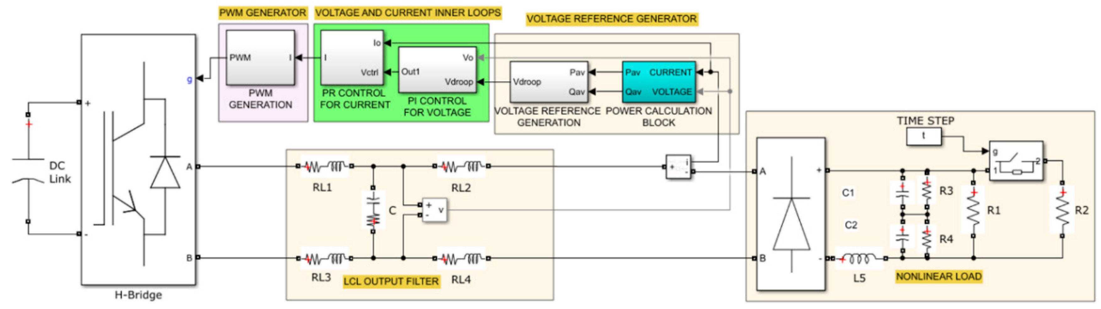
2. Materials and Methods

The scheme of a single-phase voltage source inverter (VSI) operated with the droop method when sharing a nonlinear load ZNL with another inverter is depicted in Figure 1. From the scheme, the main parts considered in this work can be seen: the power stage with inner controller, the pulse width modulation block (PWM), the LC output filter, the vo and io sensing, the Pav and Qav calculation block, and the droop generator producing the voltage reference νref [24,25]. In Figure 1, the scheme of the second inverter is not depicted. Rather, it is only outlined with discontinuous lines and indicated as #Inv. 2, due to the fact that this proposal is only concerned with the dynamic behavior and accuracy of the P-Q calculation block. For this reason, the simulations and experimental results shown from now on will only correspond to a single VSI.
In the simulations and experiments, a diode bridge rectifier (DBR) supplying a RC load is used as a nonlinear load ZNL (see Figure 2). At steady state, ZNL draws a distorted and symmetrical nonlinear current with peak levels reaching ±2.48A for the ZNL specified in Table 1, which induces a high distortion in Pav and Qav, as well as in v r e f . Likewise, a switch S1 is inserted in the ZNL scheme (see Figure 2), allowing for step-perturbations for testing the dynamic behavior of Pav and Qav and for assessment and comparison purposes.
Simulations of the proposed system for the design and comparisons with [6,17] were performed with Matlab/Simulink/Simscape Power Systems software. Table 1 shows the main parameters of the inverter and ZNL.
All the power calculation schemes were tuned to achieve the same power-ripple in order to obtain a fair comparison between the methods and to accurately measure the settling time of their transient responses when ZNL changes suddenly. The simulation results were obtained using Matlab/Simulink/Simscape Power Systems software, and were contrasted with HIL results at the inverter-based intelligent Microgrid Laboratory (iML) of the department of Energy Technology at the Aalborg University (iML-AAU) in Denmark (Figure 3).
A second similar test was performed with another diode bridge rectifier nonlinear load drawing an asymmetrical nonlinear current in order to further test the calculation power block. This current reached a peak of 4.2 A in the positive half-cycle of the VSI and a negative one of −2.2 A in the VSI negative half-cycle after an abrupt load change. This asymmetry in the current introduced an extra distortion to the calculated powers. Experimental results for this load with a VSI inverter of the iML-AAU were also obtained. The inverter used in the iMG is a Danfoss© FC302, 2.2 kW rated, interfaced to a real-time dSPACE 1006. The algorithms for operating the VSI are developed in Matlab/Simulink software and compiled into the dSPACE. Figure 4 depicts the scheme of this experimental setup.

2.1. Droop Principle-Based Control Scheme

The power calculation block of Figure 1 provides the frequency and voltage amplitude references ω * and V * , respectively, as can be seen in the following equations:
ω * = ω n m · P a v
V * = V n n · Q a v
where m and n are the droop coefficients and ω n and V n are the nominal frequency and voltage amplitude, respectively. These references are used to generate the sinusoidal voltage reference v r e f for the inverter inner control loops:
v r e f = V * · s i n ( ω * · t )
Assuming that the output voltage and current of the inverter are [15]
v o ( t ) = V · s i n ( ω o · t )
i o ( t ) = I · s i n ( ω o · t φ o )
where V and I are the voltage and current amplitudes, ω o is the fundamental frequency and φo is the phase angle between v o ( t ) and i o ( t ) , the quadrature voltage, with a −π/2 delay, is defined as
v o ( t ) = V · s i n ( ω o · t π 2 )
Therefore, the instantaneous active and reactive powers can be formulated as
p i ( t ) = v o ( t ) · i o ( t ) = V I 2 · [ c o s φ o c o s ( 2 ω o · t φ o ) ] = P a v + p ˜
q i ( t ) = v o ( t ) · i o ( t ) = V I 2 · [ s i n φ o s i n ( 2 ω o · t φ o ) ] = Q a v + q ˜
where p ˜ and q ˜ are the oscillating components that pulsate at twice the fundamental frequency ω o . These equations reveal that for a linear load that draws a sinusoidal current, the instantaneous powers oscillate around the averaged powers P a v and Q a v . However, if the load is nonlinear, the instantaneous powers are going to be highly distorted by harmonics, for which the nonlinear current can be expressed as:
i o ( t ) = I 0 · s i n ( ω o t φ o ) + h = 2 N I h · s i n ( h · ω o · t φ h )
leading to
p i ( t ) = P a v + p ˜ + v o ( t ) · h = 2 N I h · s i n ( h · ω o · t φ h )
q i ( t ) = Q a v + q ˜ + v o ( t ) · h = 2 N I h · s i n ( h · ω o · t φ h )
where the subscript h represents the harmonic order, N is the maximum considered value for h and I h , h · ω o and φ h are the amplitude, the frequency and the phase-shift of the current harmonic components, respectively. As can be seen in Equations (10) and (11), p i ( t ) and q i ( t ) contain higher harmonic order components, in addition to the DC P a v and Q a v and the double frequency components p ˜ and q ˜ that were already present in the linear case. Then, for a nonlinear ZNL, Equations (1) and (2) can be expressed as follows when they are calculated employing the instantaneous powers in Equations (10) and (11):
ω * ( t ) = ω n m · ( P a v + p ˜ + v o ( t ) · h = 2 N I h · s i n ( h · ω o · t φ h ) )
V * ( t ) = V n n · ( Q a v + q ˜ + v o ( t ) · h = 2 N I h · s i n ( h · ω o · t φ h ) )
and the voltage reference is
v r e f ( t ) = V * ( t ) · s i n ( ω * ( t ) · t )

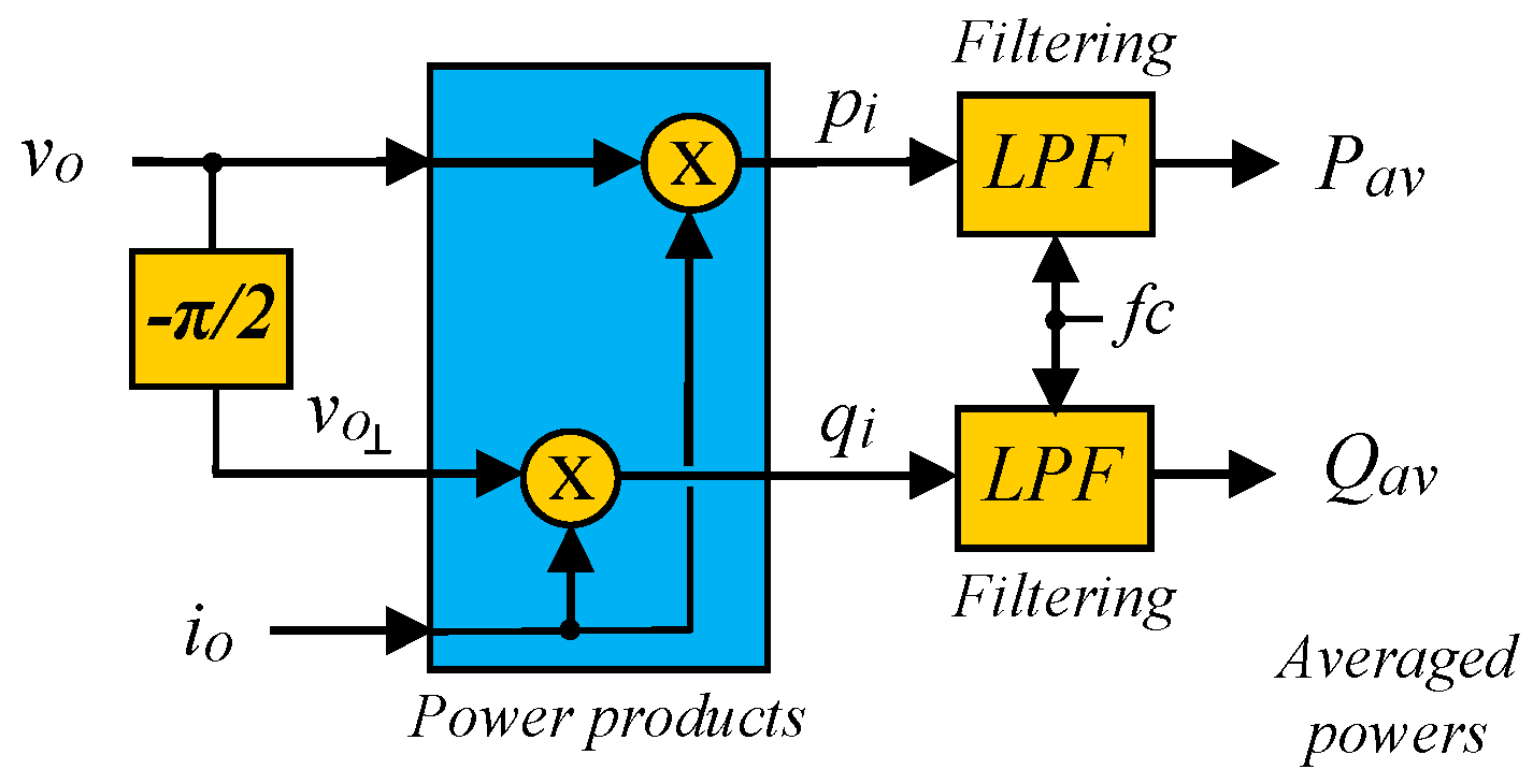
2.2. Conventional P-Q Calculation Schemes

Figure 5 shows the conventional P-Q calculation scheme for obtaining P a v and Q a v , in which the instantaneous powers p i ( t ) and q i ( t ) are obtained as the products of i o ( t ) with v o ( t ) and v o ( t ) , respectively [6]. The quadrature voltage v o ( t ) is obtained by delaying v o ( t ) by π/2, and P a v and Q a v by using LPFs with a low cut-off frequency value fc, to filter the multiple frequency components in the instantaneous powers [18]. When sharing linear loads, the value of fc is usually set to one or two orders of magnitude lower than the inverter fundamental operating frequency [22,23], which determines the transient dynamic performance of the system. However, in the case of nonlinear loads, the value of fc should be further reduced (usually to less than 1 Hz), to avoid strong distortions in the inverter output current and in the instantaneous powers [24]. Conversely, the distortion in the current induces excessive ripple in the averaged powers, which in turn is translated to the droop references ω * ( t ) and V * ( t ) , and then to v r e f ( t ) , causing bad operation of the system. Nevertheless, this bandwidth reduction slows down the transient dynamic behavior of the system. The transfer functions of the averaged P a v and Q a v are shown in Appendix A.

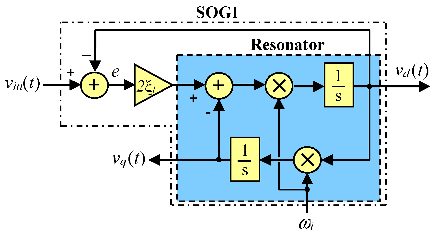
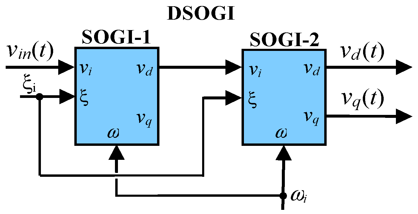
2.3. The SOGI and DSOGI Approach

A SOGI is a special linear filter with one input, vin(t), and two outputs, vd (t) and vq(t), one in phase and the other delayed π/2 with respect to the input, respectively, see Figure 6.
The outputs of the SOGI filter, vd(t) and vq(t), have the following band-pass filter (BPF) and LPF transfer function relationships regarding to the input:
H d ( s ) = v d ( s ) v i n ( s ) = 2 ξ i ω i · s s 2 + 2 ξ i ω i · s + ω i 2 H d ( s ) = v d ( s ) v i n ( s ) = 2 ξ i ω i · s s 2 + 2 ξ i ω i · s + ω i 2
H q ( s ) = v q ( s ) v i n ( s ) = 2 ξ i ω i 2 s 2 + 2 ξ i ω i · s + ω i 2 H q ( s ) = v q ( s ) v i n ( s ) = 2 ξ i ω i 2 s 2 + 2 ξ i ω i · s + ω i 2
where ξi is the filter damping factor and ωi is the tuning center frequency. In addition, a DSOGI is a four-order filter that consist in the cascade connection of two SOGI filters, as seen in Figure 7 [26]:
The transfer functions of the DSOGI with respect to the input [26]:
H d ( s ) = ( 2 ξ i ω i · s s 2 + 2 ξ i ω i · s + ω i 2 ) 2
H q ( s ) = 4 ξ i 2 ω i 3 · s ( s 2 + 2 ξ i ω i · s + ω i 2 ) 2
When ωi is tuned to match ω o , and for harmonic components higher than the fundamental (h 1 ) , the gain of the BPF characteristic in Equation (17) can be simplified to:
| H d ( s ) | = ( 2 ξ i h ( 1 h 2 ) 2 + ( 2 ξ i h ) 2 ) 2 ( 2 ξ i h ) 2 | H d ( s ) | = ( 2 ξ i h ( 1 h 2 ) 2 + ( 2 ξ i h ) 2 ) 2 ( 2 ξ i h ) 2
On the other hand, the frequency and damping factor are the parameters that determine the settling time t s (2% criterion) of the transient response of the BPF in Equation (15) for a step input:
t s 4 ξ i · ω i
The SOGI filter has an inherent trade-off relationship between bandwidth (rejection capability to harmonics) and settling time response, Equation (20). This trade-off cannot be overcome, and relies on the damping factor parameter ξ i . However, in [26], it was shown that the DSOGI has a better trade-off than the SOGI and can achieve a faster transient response when it is designed to have the same bandwidth behavior. In this paper, this characteristic is used to achieve a faster response when extracting the fundamental component of the nonlinear load current and thereby to improve the droop transient response to load changes.

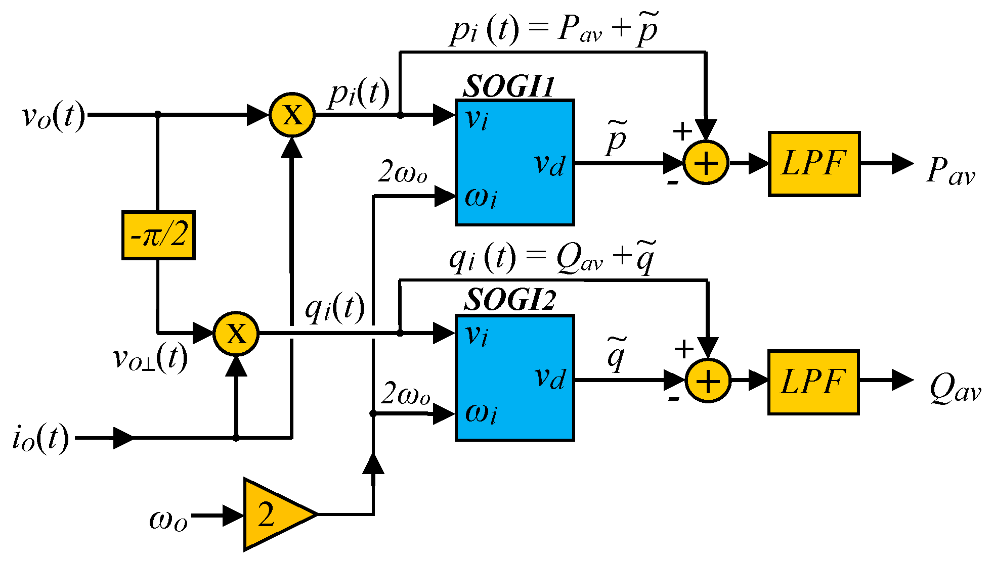
2.4. Advanced P-Q Calculation Scheme

Figure 8 shows a P-Q calculation method based on the proposed scheme in [17] for accelerating the computation of Pav and Qav. In this figure, the SOGI1 and SOGI2 blocks are used for extracting the double frequency pulsating power components p ˜ and q ˜ , which are then removed from pi and qi. These SOGIs are both tuned at ω i = 2 ω o and ξ 1 = ξ 2 = 1 . The LPFs are used for improved filtering and for providing the averaged powers Pav and Qav, by attenuating the higher harmonics components reported in Equations (10) and (11). This figure does not show the method for generating the π/2 delay, since it is not mentioned in [17]. Therefore, another SOGI, SOGI0, tuned at ω o and ξ 0 = ξ v = 0.707 , is used for generating this delay, as shown in Figure 9, for avoiding the delay issues reported in [15,16].
The transfer functions for the calculated averaged active and reactive power are included in Appendix A, with the numbers (24) and (25). Please note that the current is not filtered.
Figure 10 shows the simulation results using the P-Q algorithms of the schemes in Figure 5 and Figure 9 when sharing a linear load that produces a current perturbation from peak 2A to peak 4A at a time of 3 s.
For the sake of simplicity, Figure 10 only shows the dynamic behavior of Pav, obviating the representation of Qav. The dynamics of Pav obtained with the advanced scheme in Figure 9 (hereinafter called Padv) are compared with those obtained for Pav by the conventional droop method depicted in Figure 5 (hereinafter called Pdroop). The cut-off frequency of the LPFs in Figure 9 was designed to be fc = 3.7 Hz, whereas it was set to fc = 0.37Hz for the scheme in Figure 5. As shown in Figure 10, the double frequency component p ˜ was removed from Padv. Likewise, the higher cut-off frequency of its LPFs results in much faster dynamics than those of Pdroop. Also, the ripple corresponding to the double frequency component p ˜ , which is not completely filtered by the LPFs in Figure 5, can be observed in Pdroop. These results are compatible with those reported in [21]. However, the good dynamic behavior depicted in Figure 10 for Padv vanishes when a nonlinear load is used, as is shown in Figure 11. In this case, the nonlinear load is a DBR that draws a peak current of ±2.48 A and suffers a perturbation that pushes the peak to ±4.15 A. The simulation parameters are listed in Table 2.
As shown in Figure 11, the dynamics of the method proposed in [20] worsen using a nonlinear load, similarly to [26]. Thus, in the presence of a nonlinear load, the method has excessive steady state ripple that corrupts the calculated powers, opposite to what is stated in [20]. To reduce the ripple, the filtering capabilities of the LPFs in Figure 9 can be improved by reducing fc. By decreasing fc from 3.7 Hz to 1.1 Hz, the ripple of Padv matches that of Pdroop, as can be seen in Figure 12. Although the advanced method of Figure 9 calculates faster Pav than the conventional droop controller, it presents less effectivity than initially argued. It can be clearly seen in Figure 11 and Figure 12 that there is a trade-off between the filtering capability of the Pav calculation scheme and the transient speed of its dynamical response. Note also that there is a positive offset in the calculated Pav at steady state, since the mean value of Padv is slightly higher than that of Pdroop (see Figure 11). Comparing the transfer functions for the P-Q calculation by the conventional, Equations (22) and (23), or by the advanced method, Equations (24) and (25), it can be seen the filtering capabilities of each algorithm. Please note that the magnitude of the ripple of Padv forces the system’s dynamic response to slow down by reducing more the cut-off frequency.

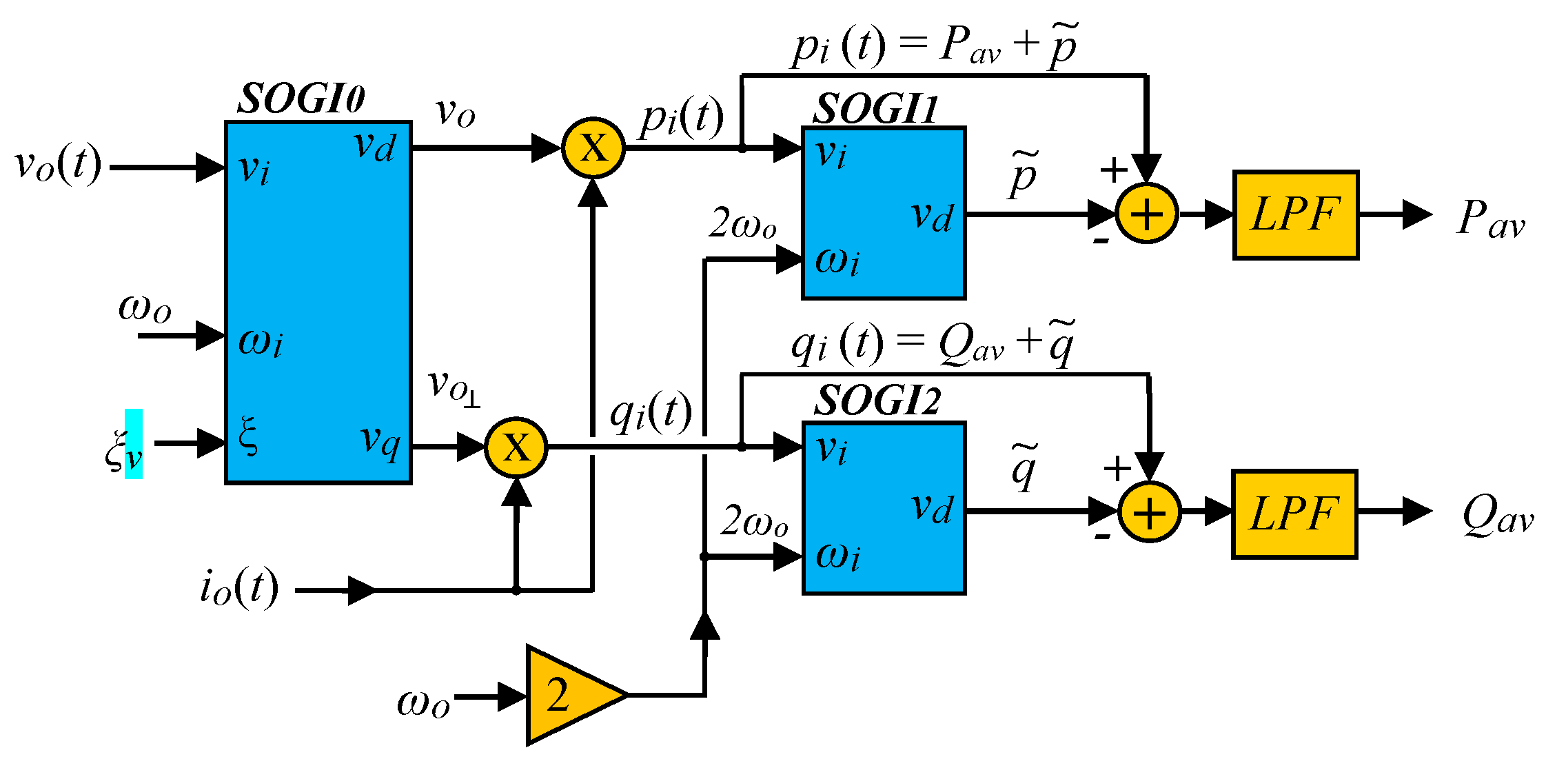
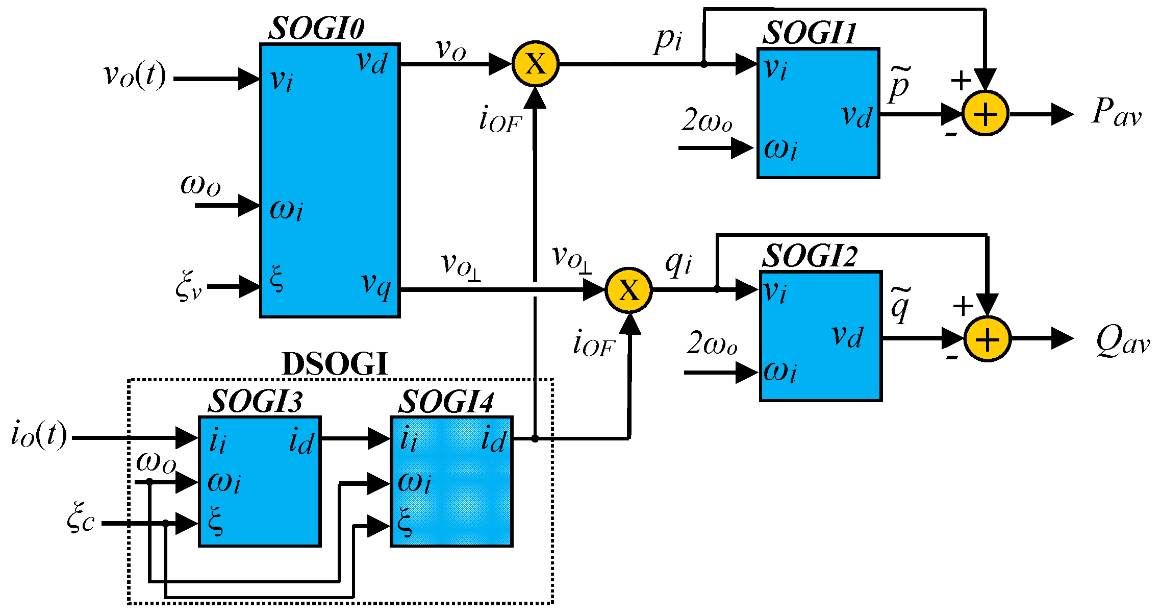
2.5. Proposed P-Q Calculation Scheme

The scheme of the proposed P-Q calculation is shown in Figure 13. A DSOGI approach is applied to i o ( t ) in order to extract the fundamental component i O F , see Equation (28) in Appendix A. There, the DSOGI composed of the SOGI3 and SOGI4 blocks filters the distorting high-order harmonics of i o ( t ) by means of its higher BPF capability and avoids coping with a highly distorted current signal. Consequently, the instantaneous powers p i ( t ) and q i ( t ) are obtained as the product of the in-phase v o ( t ) or the quadrature v o ( t ) voltages with the fundamental output current iOF, respectively. This produces a result with only double frequency components and without third or higher order harmonics.
Later, the SOGI1 and SOGI2 blocks were used as in Figure 9 for removing only the double frequency components with the help of the subtracting blocks. Therefore, the LPFs can now be removed from the scheme, since they are no longer necessary. The transfer function of the proposed scheme in Figure 13 is shown in Appendix A as Equations (26) and (27). This overcomes the main limitation of previous schemes and further accelerates the dynamic response of Pav and Qav. To distinguish Pav and Qav obtained with this proposed scheme, in the following they will be referred to as PDSOGI and QDSOGI.
In this case, because a DSOGI is used for filtering the current in Equation (28), and considering that the center frequencies provided by the droop method ω* vary in a small range around the nominal frequency ωn, the transient response speed is determined mainly by the DSOGI transient response, which is related to ξ c ; see [26]. The damping factors of the DSOGI are here tuned to produce a power ripple identical in amplitude to that of the conventional droop controller, which is achieved for ξc = ξ3= ξ4 = 0.129.
Figure 14 shows the simulation results of the same nonlinear DBR load drawing a peak current of ±2.48 A and suffering a perturbation that pushes the peak to ±4.15 A. It can be observed that the proposed method is faster for calculating Pav than the previously considered methods.
Figure 15 depicts the simulation results using a ZNL drawing an asymmetrical current, reaching a positive peak of 5.21 A and a negative peak of −3.07 A after the perturbation. In this case, the asymmetry in the nonlinear current (see Figure 15a), introduces further distortion into the calculated Pav, showing higher ripple at steady state (see Figure 15c).
Please note that unlike Padv, PDSOGI does not exhibit a positive offset error in steady state. This means that the proposed method is also more accurate than that in [20]. Table 3 contains the measured settling time for the Pav transient responses depicted in Figure 15, which shows that the PDSOGI calculated with the proposed method implies a 60.00% and a 79.69% reduction in the response time regarding Padv and Pdroop, respectively.

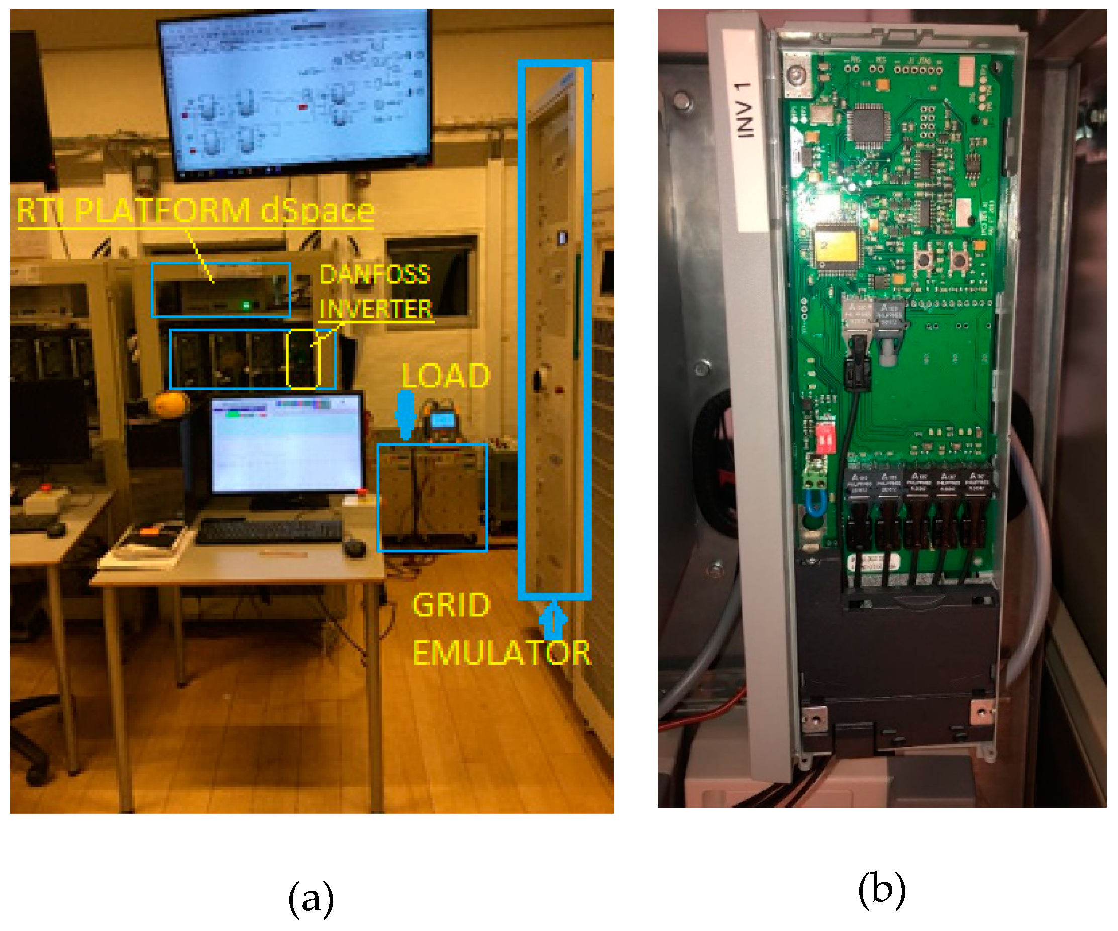
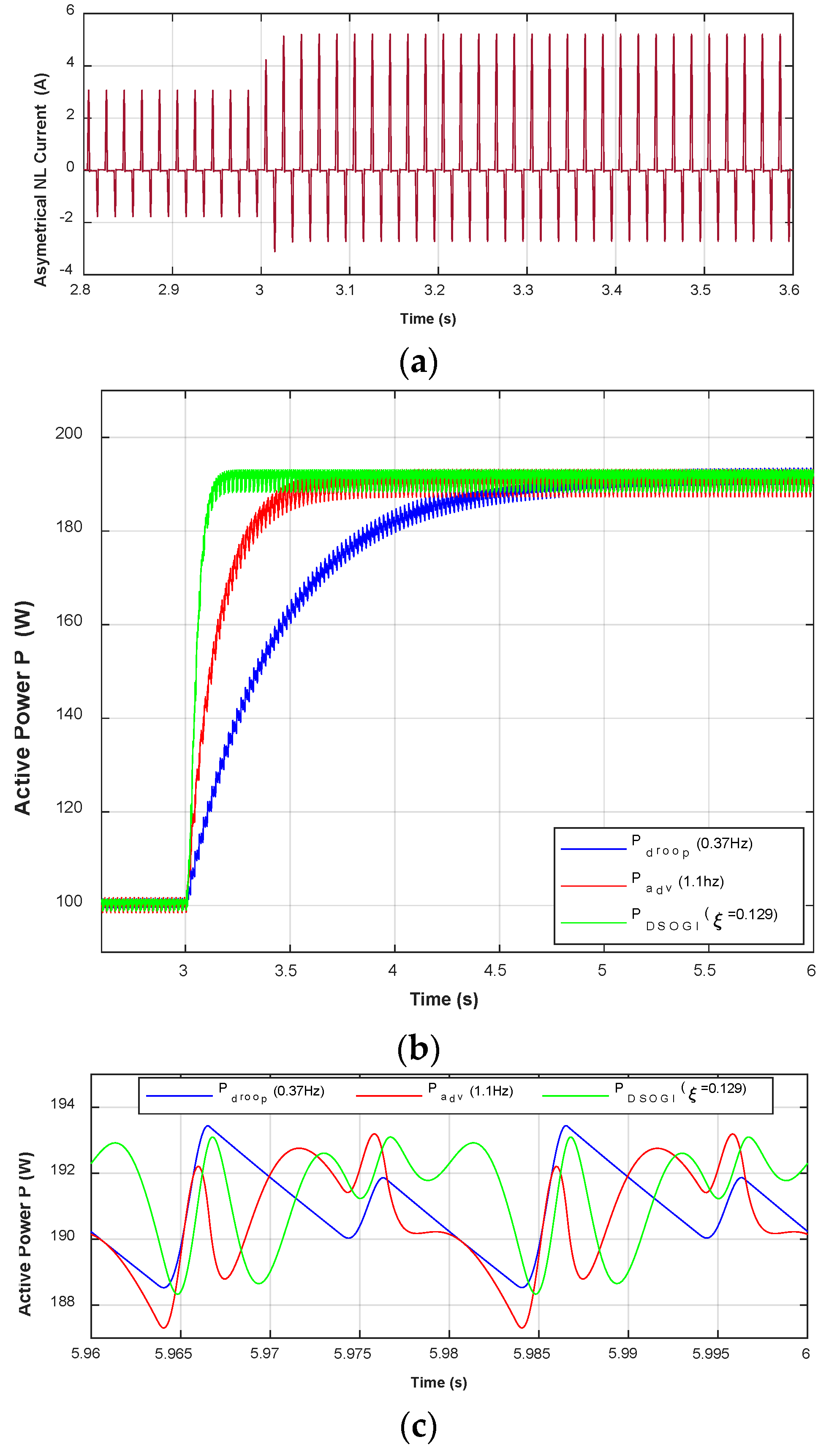
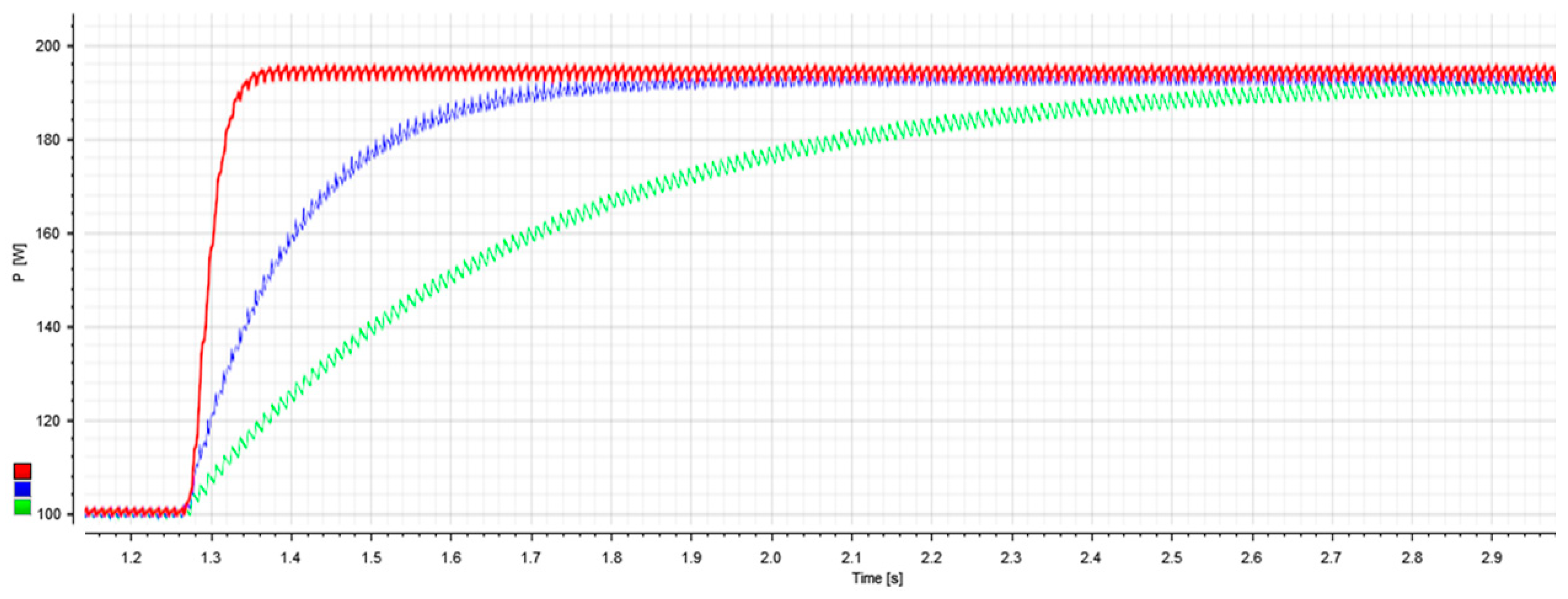
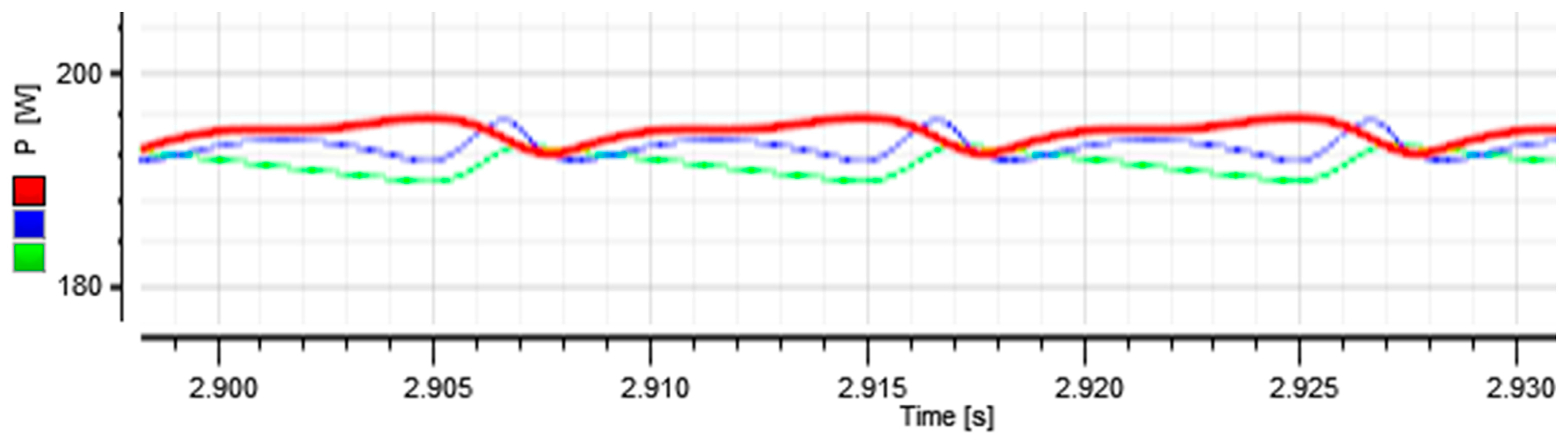
3. Experimental Results

Hardware in Loop, as well as experimental results with an VSI inverter of the iML-AAU, were obtained. The HIL setup consisted of a dSpace 1006© digital Real-Time Interface platform that carried out the processor-based simulations with parameters configured by the dSpace Configuration Desk © tool. The setup supports models based on the physical modelling libraries of electrical plants designed by Matlab/Simulink/SimPowerSystems©. These models are integrated into the dSpace tool chain and are used for building the electrical system under test along with the Electronic Central Unit, ECU, of the dSpace. The control algorithms described in this paper were loaded and executed in real time in the ECU. In this case, the H-Bridge Inverter, the LCL filter and the Nonlinear Load depicted in Figure 4 are the electrical system implemented in the ECU under the HIL test. The experimental setup consisted of an inverter Danfoss© FC302, 2.2 kW rated, interfaced to the real-time dSPACE 1006 digital platform. The algorithms for operating the VSI were developed in Matlab/Simulink software and compiled in the dSPACE multiprocessor core, with its parameters configured and controlled through the Configuration-Desk software. The sampling frequency for the system was 10 kHz, which was the switching frequency for the VSI. A third-order method for discretizing the SOGI and DSOGI algorithms was employed, whereby the integrator 1 s   was approximated as:
T s 12 · 5 z 3 16 z 2 + 23 z 1 1 z 1
with Ts being the sample time of 100 µs, which is consistent with the 10 kHz frequency. The experimental setup parameters for the LCL filter and for the nonlinear load are listed in Table 4.
In this section, HIL results are shown first for a ZNL drawing a symmetrical current, and then the results for a VSI with a ZNL drawing an asymmetrical current.
Figure 16 depicts the HIL Pav results for a ZNL drawing a symmetrical current with peak values transitioning from ±2.48 A to ±4.15 A after a step perturbation at 1.28 s. The dynamics of Pav obtained with the different considered methods are represented in green for Pdroop, in blue for Padv and in red for PDSOGI.
Figure 17 shows a detail of the Pav ripple waveforms at steady state, evidencing the different nonlinearities resulting from each power calculation method. There are some DC errors in the calculated powers that can mainly be attributed to the discretization method in Equation (21) and to the sampling frequency. This phenomenon was not evidenced in the simulations shown in Figure 15c, but is reflected in the HIL results.
Figure 18 shows the output voltage vo(t) waveform of the VSI (Figure 18a), the current waveform drawn for the DBR load and used for obtaining the VSI results (Figure 18b) and the fundamental current component iOF extracted by the DSOGI (Figure 18c). Note the current asymmetry, with positive peaks that reach 4.2 A and negative ones that reach −2.8 A. Note how a fundamental current component t of 1.5 A amplitude has been achieved.
Finally, Figure 19 depicts the Pav experimental VSI results with the DBR load when a perturbation is applied at 8.9 s. Note in this figure that the results are coherent with those obtained by HIL, as shown in Figure 16, and by the simulations in Figure 15.
Table 5 presents the settling time of Pav obtained with all the considered P-Q calculation methods, as measured in Figure 15 for Matlab/Simulink® simulations results, in Figure 16 for the HIL results, and in Figure 19 for the experimental VSI results. In this table, the achieved percentage of settling time reduction with respect to the conventional droop method is also indicated. Note how the proposed method achieves a faster response. The transfer functions for the active and reactive averaged powers of the droop, advanced and DSOGI methods are shown in Appendix A.

4. Discussion

In this work, a P-Q calculation method was proposed for single-phase inverters with the purpose of improving the speed and accuracy of the power calculation when they are sharing linear and nonlinear loads. The dynamic response of the power calculation used in the conventional droop method and in another advanced method was first analyzed to show their limitations in speed and accuracy when sharing a DBR-type nonlinear load. For this reason, a novel calculation method was proposed, bearing in mind the dynamic transient response velocity of the system to sudden perturbations in the shared load. The method was studied and compared with previous ones by obtaining results from Matlab®-based simulations, the HIL platform, and a VSI experimental setup. These results show how the proposed method achieves, under the same distorting conditions, a faster calculation settling time with a measured time reduction over the conventional droop method that arrives around 80%, which is higher than the achieved by the advanced method. This improvement supposes an enhancement in the droop speed operation under linear and nonlinear load conditions that leads to a better dynamic performance of the system when parallelizing inverters or microgrid operation in islanded mode.
The aim of this work was to identify what the main limitation of the power calculation methods was for sharing linear and nonlinear loads, and to propose a new approach based on the DSOGI scheme. This issue can be further investigated by using the SOGI approach and other ones for obtaining the fundamental component of the distorted current signals with less effort, faster, and best quality. This would help in the operation and stability of the inverters when sharing linear and nonlinear loads.

Author Contributions

Investigation, simulation results and writing—original draft, J.E.M. and J.M.; methodology and formal analysis, J.E.M., J.M., H.M. and J.M.G.; writing—review and editing, J.E.M., J.M., H.M.; writing—response to reviewers, J.M. and H.M.; software design, J.E.M., J.M. and M.L.; laboratory setup, HIL and experimental results, J.E.M., M.L., and Y.G.; data curation, J.E.M., J.M. and M.L.; laboratory organization and supervision, J.M.G.

Funding

J. M. Guerrero was funded by a Villum Investigator grant (no. 25920) from The Villum Fonden.

Acknowledgments

Thanks to Alexander Micallef, University of Malta, for his crucial support during the experimental campaign. Thanks also to the E3PACS laboratory staff from UPC, that provided technical support during the redaction of this work.

Conflicts of Interest

The authors declare no conflict of interest.

Appendix A

The transfer functions of the active and reactive averaged powers regarding the instantaneous powers of the methods described here are as follows:
P d r o o p ( s ) = ( ω c s + ω c ) p i ( s )
Q d r o o p ( s ) = ( ω c s + ω c ) q i ( s )
P a d v ( s ) = ( s 2 + ( 2 ω o ) 2 s 2 + 2 ( 2 ω o ) · s + ( 2 ω o ) 2 ) ( ω c s + ω c ) p i ( s )
Q a d v ( s ) = ( s 2 + ( 2 ω o ) 2 s 2 + 2 ( 2 ω o ) · s + ( 2 ω o ) 2 ) ( ω c s + ω c ) q i ( s )
P D S O G I ( s ) = ( s 2 + ( 2 ω o ) 2 s 2 + 2 ( 2 ω o ) · s + ( 2 ω o ) 2 ) p i ( s )
Q D S O G I ( s ) = ( s 2 + ( 2 ω o ) 2 s 2 + 2 ( 2 ω o ) · s + ( 2 ω o ) 2 ) q i ( s )
where ω c = 2 π f c is the cut-off frequency in rad/s of the LPFs used in the droop- and advanced-based methods. The instantaneous powers, p i ( t ) and q i ( t ) , are derived from the product between i o ( t ) and v o ( t ) and v o ( t ) , respectively. The transfer functions for v o ( t ) and v o ( t ) correspond to Equations (15) and (16) in all the methods, since a SOGI was used to achieve these signals. In addition, in the case of the current, the fundamental component i O F in the DSOGI method has the following transfer function:
i O F ( s ) = ( 2 ξ c ω o · s s 2 + 2 ξ c ω o · s + ω c 2 ) 2 i o ( s )

References

  1. Kim, J.-H.; Lee, Y.-S.; Kim, H.-J.; Han, B.-M. A New Reactive-Power Sharing Scheme for Two Inverter-Based Distributed Generations with Unequal Line Impedances in Islanded Microgrids. Energies 2017, 10, 1800. [Google Scholar] [CrossRef]
  2. Ren, B.; Sun, X.; Chen, S.; Liu, H. A Compensation Control Scheme of Voltage Unbalance Using a Combined Three-Phase Inverter in an Islanded Microgrid. Energies 2018, 11, 2486. [Google Scholar] [CrossRef]
  3. Ma, J.; Wang, X.; Liu, J.; Gao, H. An Improved Droop Control Method for Voltage-Source Inverter Parallel Systems Considering Line Impedance Differences. Energies 2019, 12, 1158. [Google Scholar] [CrossRef]
  4. Coelho, E.A.A.; Cortizo, P.C.; Garcia, P.F.D. Small signal stability for single phase inverter connected to stiff AC system. In Proceedings of the Record of the IEEE Industry Applications Conf. 34th IAS Annual Meeting (Cat. No.99CH36370), Phoenix, AZ, USA, 1999; Volume 4, pp. 2180–2187. [Google Scholar]
  5. Soshinskaya, M.; Graus, W.H.J.; Guerrero, J.M.; Vasquez, J.C. Microgrids: experiences barriers and success factors. Renew. Sustain. Energy Rev. 2014, 40, 659–672. [Google Scholar] [CrossRef]
  6. Araújo, L.S.; Narváez, D.I.; Siqueira, T.G.; Villalva, M.G. Modified droop control for low voltage single phase isolated microgrids. In Proceedings of the IEEE Int. Conf. on Automatica (ICA-ACCA), Curico, Chile, 19–21 October 2016; pp. 1–6. [Google Scholar]
  7. IEEE. IEEE Standard Definitions for the Measurement of Electric Power Quantities Under Sinusoidal, Nonsinusoidal, Balanced or Unbalanced Conditions; IEEE Standard 1459-2010; IEEE: New York, NY, USA, 2000; pp. 1–52. [Google Scholar]
  8. Lu, J.; Wen, Y.; Zhang, Y.; Wen, W. A novel power calculation method based on second order general integrator. In Proceedings of the IEEE 8th Int. Power Electronics and Motion Control Conf. (IPEMC-ECCE Asia), Hefei, China, 22–26 May 2016; pp. 1975–1979. [Google Scholar]
  9. Andrade, E.T.; Ribeiro, P.E.M.J.; Pinto, J.O.P.; Chen, C.L.; Lai, J.S.; Kees, N. A novel power calculation method for droop-control microgrid systems. In Proceedings of the 2012 27th Annual IEEE Applied Power Electronics Conf. and Exp. (APEC), Vladivostok, Russia, 9–10 September 2012; pp. 2254–2258. [Google Scholar]
  10. Ren, Z.; Gao, M.; Mo, Q.; Liu, K.; Yao, W.; Chen, M.; Qian, Z. Power Calculation Method Used in Wireless Parallel Inverters Under Nonlinear Load Conditions; IEEE: New York, NY, USA, 2010. [Google Scholar]
  11. Furtado, E.C.; Aguirre, L.A.; Torres, L.A.B. UPS Parallel Balanced Operation Without Explicit Estimation of Reactive Power—A Simpler Scheme. In Circuits and Systems II: Express Briefs; IEEE Trans. Eds.; IEEE: New York, NY, USA, 2008; pp. 1061–1065. [Google Scholar]
  12. Guerrero, J.; Matas, J.; Vicuna, L.G.; Castilla, M.; Miret, J. Decentralized Control for Parallel Operation of Distributed Generation Inverters Using Resistive Output Impedance. In Industrial Electronics; IEEE Trans. Eds.; IEEE: New York, NY, USA, 2007; pp. 994–1004. [Google Scholar]
  13. Silva, S.A.; Novochadlo, R.; Modesto, R.A. Single-phase PLL structure using modified p-q theory for utility connected systems. In Proceedings of the IEEE PESC, Rhodes, Greece, 15–19 June 2008; pp. 4706–4711. [Google Scholar]
  14. Wang, H.; Yue, X.; Pei, X.; Kang, Y. A new method of power calculation based on parallel inverters. In Proceedings of the IEEE EPE-PEMC, Novi Sad, Serbia, 28–30th October 2009; pp. 1573–1576. [Google Scholar]
  15. Wei, Y.; Xu, D.; Ma, K. A Novel Accurate Active and Reactive Power Calculation Method for Paralleled UPS System. In Proceedings of the APEC, Singapore, 15–16 November 2009; pp. 1269–1275. [Google Scholar]
  16. Ren, Z.; Gao, M.; Mo, Q.; Liu, K.; Yao, W.; Chen, M.; Qian, M. Power calculation method used in wireless parallel inverters under nonlinear load conditions. In Proceedings of the 25th Annual IEEE Applied Power Electronics Conf. and Exp., Palm Springs, CA, USA, 21–25 February 2010; pp. 1674–1677. [Google Scholar]
  17. Akagi, H.; Watanabe, E.; Aredes, M. Instantaneous Power Theory and Application to Power Conditioning; IEEE Press Series in Power Engineering; IEEE: New York, NY, USA, 2007; pp. 5–28. [Google Scholar]
  18. Gao, M.; Yang, S.; Jin, C.; Ren, Z.; Chen, M.; Qian, Z. Analysis and experimental validation for power calculation based on p-q theory in single-phase wireless-parallel inverters. In Proceedings of the 26th Annual IEEE Applied Power Electronics Conference and Exposition (APEC), Hyderabad, India, 16–18 December 2011; pp. 620–624. [Google Scholar]
  19. Matas, J.; Castilla, M.; d. Vicuña, L.G.; Miret, J.; Vasquez, J.C. Virtual Impedance Loop for Droop-Controlled Single-Phase Parallel Inverters Using a Second-Order General-Integrator Scheme. In Power Electronics; IEEE Trans. Eds.; IEEE: New York, NY, USA, 2010; pp. 2993–3002. [Google Scholar]
  20. Tolani, S.; Sensarma, P. An improved droop controller for parallel operation of single-phase inverters using R-C output impedance. In Power Electronics, Drives and Energy Systems (PEDES), Bengaluru; IEEE Trans. Eds.; IEEE: New York, NY, USA, 2012; pp. 1–6. [Google Scholar]
  21. Yang, Y.; Blaabjerg, F. A new power calculation method for single-phase grid-connected systems. In IEEE International Symposium on Industrial Electronics; IEEE Eds.; IEEE: New York, NY, USA, 2013; pp. 1–6. [Google Scholar]
  22. Guerrero, J.M.; Berbel, N.; Matas, J.; de Vicuna, L.G.; Miret, J. Decentralized Control for Parallel Operation of Distributed Generation Inverters in Microgrids Using Resistive Output Impedance. In Proceedings of the IECON 2006—32nd Annual Conference on IEEE Industrial Electronics, Paris, France, 7–10 November 2006; pp. 5149–5154. [Google Scholar]
  23. Mariachet, J.E.; Matas, J.; Martín, H.; Abusorrah, A. Power Calculation Algorithm for Single-Phase Droop-Operated Inverters Considering Nonlinear Loads. Renew. Energy Power Qual. J. 2018, 1, 16. [Google Scholar]
  24. Song, H.; Nam, K. Dual current control scheme for PWM converter under unbalanced input voltage conditions. In Ind. Electron; IEEE Trans. Eds.; IEEE: New York, NY, USA, 1991; pp. 953–959. [Google Scholar]
  25. IEEE Standard Definitions for the Measurement of Electric Power Quantities Under Sinusoidal; Nonsinusoidal, Balanced, or Unbalanced Conditions-Redline; IEEE: New York, NY, USA, 2010; pp. 1–52, 1459-2010 (Revision of IEEE Std 1459-2000)-Redline, 19 March 2010.
  26. Matas, J.; Castilla, M.; Miret, J.; Vicuna, L.G.; Guzman, R. An adaptive prefiltering method to improve the speed/accuracy tradeoff of voltage sequence detection methods under adverse grid conditions. IEEE Trans. Ind. Electron. 2014, 61, 2139–2151. [Google Scholar] [CrossRef]
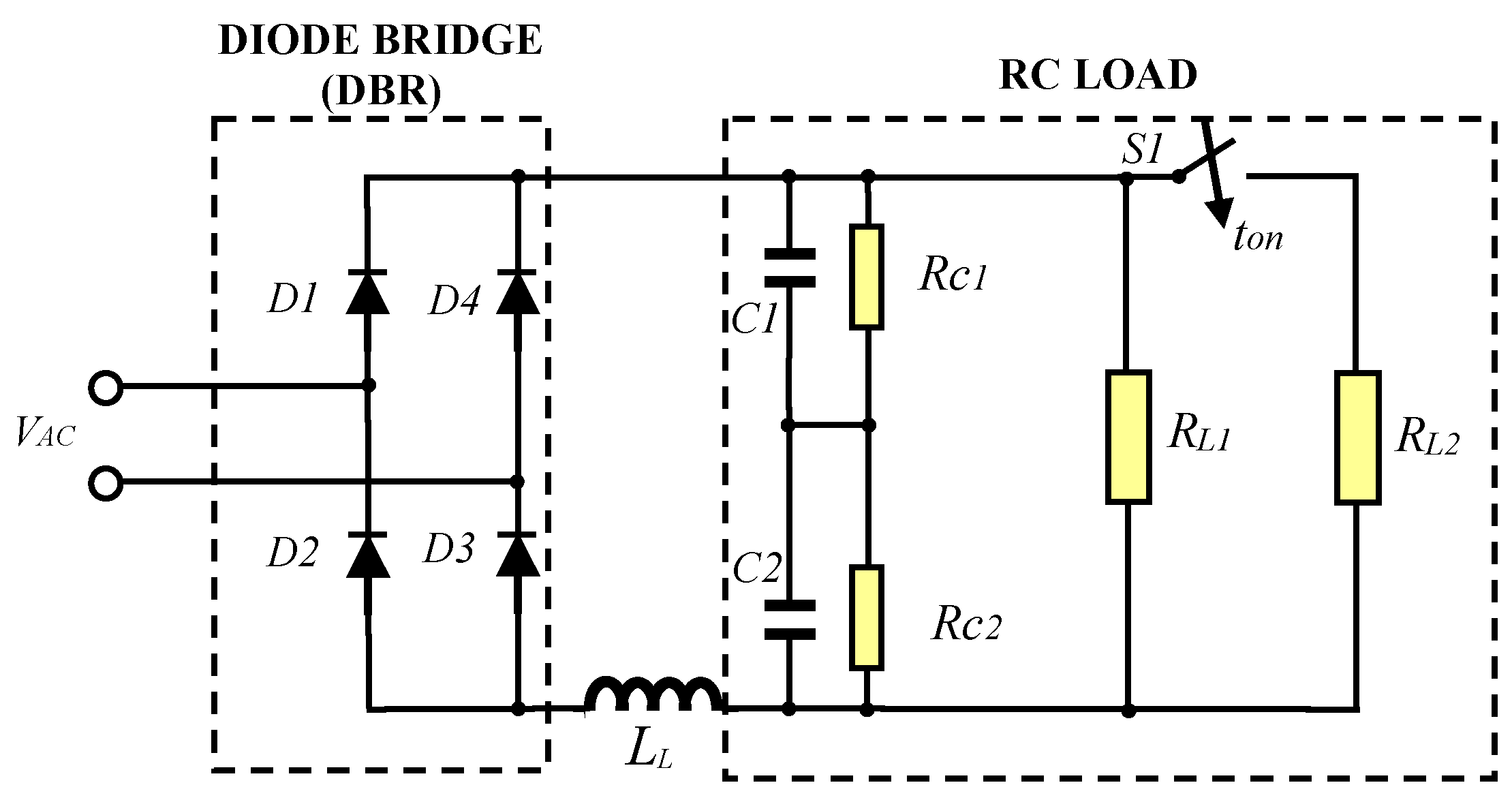
Figure 1. Block scheme of a single-phase voltage source inverter (VSI) (Inv. #1) sharing a nonlinear load with a second inverter (Inv. #2) and showing the P-Q power calculation, the Droop Generator and the PWM (pulse width modulation) control blocks.
Electronics 08 01366 g001
Figure 2. Diode-bridge rectifier nonlinear load supplying a resistive-capacitive load.
Electronics 08 01366 g002
Figure 3. Experimental setup at the intelligent Microgrid Laboratory in Aalborg University (iML-AAU), Denmark: (a) Complete experimental setup; (b) detail of the Danfoss© single-phase inverter.
Electronics 08 01366 g003
Figure 4. Scheme of the VSI experimental setup implemented at the iMG_AAU.
Electronics 08 01366 g004
Figure 5. Block diagram of conventional P-Q power calculation providing the averaged powers Pav and Qav.
Electronics 08 01366 g005
Figure 6. Block diagram of the SOGI (second-order generalized integrator) filter.
Electronics 08 01366 g006
Figure 7. Block diagram of a DSOGI (double SOGI) filter as the cascading of two individual SOGIs.
Electronics 08 01366 g007
Figure 8. Scheme for the calculation of Pav and Qav proposed in [20].
Electronics 08 01366 g008
Figure 9. Addition to Figure 8 of a new SOGI for archiving the quadrature component of the output voltage vo(t).
Electronics 08 01366 g009
Figure 10. Simulation of the load current and Pav transient responses for a linear load current perturbation from peak 2A to peak 4A at 3 s: (a) detail of the load current perturbation, (b) comparison between Pav obtained with Figure 9 scheme (Padv) and Pav obtained with Figure 5 scheme (Pdroop).
Electronics 08 01366 g010
Figure 11. Simulation of the load current and Pav transient responses for a nonlinear Diode Bridge Rectifier (DBR) load current perturbation from a peak at 2.48 A to a peak at 4.15 A at 3 s: (a) detail of the distorted load current perturbation, (b) Padv and Pdroop, (c) detail of Padv and Pdroop ripples.
Electronics 08 01366 g011aElectronics 08 01366 g011b
Figure 12. Simulation of the Pav transient responses for a nonlinear DBR (diode bridge rectifier) load current perturbation from a peak at 2.48 A to a peak at 4.15 A at 3 s: (a) Padv (with reduced fc = 1.1 Hz) and Pdroop, (b) detail of Padv and Pdroop ripples.
Electronics 08 01366 g012
Figure 13. Scheme for the proposed P-Q calculation based on a DSOGI approach.
Electronics 08 01366 g013
Figure 14. Simulation of iOF and Pav transient responses for a nonlinear DBR load current perturbation from a peak of 2.48 A to 4.15 A at 3 s: (a) detail of the iOF perturbation, (b) PDSOGI, Padv and Pdroop, (c) detail of PDSOGI, Padv and Pdroop ripples.
Electronics 08 01366 g014
Figure 15. Simulation of the load current and Pav transient responses for an asymmetrical nonlinear DBR load current with a positive peak of 5.21 A and a negative peak of −3.07 A after the perturbation at 3 s: (a) detail of the asymmetrical load current perturbation, (b) PDSOGI, Padv and Pdroop, (c) detail of PDSOGI, Padv and Pdroop ripples.
Electronics 08 01366 g015
Figure 16. HIL Pav results for a ZNL drawing a symmetrical current with peak values from ±2.48 A to ±4.15 A after a step perturbation at 1.28 s (Pdroop in green, Padv in blue, PDSOGI in red).
Electronics 08 01366 g016
Figure 17. Detail of HIL Pav ripples at steady-state from Figure 14 (Pdroop in green, Padv in blue, PDSOGI in red).
Electronics 08 01366 g017
Figure 18. VSI output voltage and asymmetrical current waveforms drawn by the nonlinear DBR load used to obtain the VSI results. (a) Output voltage, vo(t); (b) asymmetrical nonlinear current; (c) fundamental component iOF extracted by the DSOGI.
Electronics 08 01366 g018
Figure 19. VSI experimental result of the Pdroop transient response for the nonlinear DBR load current perturbation in Figure 18 (Pdroop in green, Padv in blue, PDSOGI in red).
Electronics 08 01366 g019
Table 1. Main parameters of VSI and ZNL.
ParameterValue
LC Filter1.8 mH; 25 µF
Switching frequency, fs10 kHz
RonD1-D40.01 Ω
L L 84 µH
C1, C2470 µF
R C 1 ,   R C 2 37 kΩ
R L 1 ,   R L 2 960 Ω
Table 2. Simulation parameters for Figure 10.
ParameterValue
Vn311 V
ωo2π50 rad/s
DBR RESISTOR LOAD FOR T < 3S950 Ω
DBR RESISTOR LOAD FOR T > 3S471.8 Ω
THD io(t) 215%
ξ00.7
ξ1 = ξ21
Table 3. Settling time simulation measurements from Figure 15.
ParameterValue
PDROOP325 ms
PADV165 ms
PDSOGI66 ms
Table 4. Main parameters of VSI and ZNL.
ParameterValue
RL1 = RL2 = RL3 = RL41.8 mH; 0.01 Ω
RC branch25 µF; 1 Ω
Switching frequency, fs10 kHz
RonD1 and D4/ RonD2 and D30.01 Ω/ 1 Ω
LL84 µH
C1 = C2/ Rc1 = Rc2470 µF/37 kΩ
R L 1 ,   R L 2 960 Ω
Table 5. Experimental results for the VSI setup.
P-Q
Algorithm
Settling Time
Matlab (ms)/(%reduction)
Settling Time
HIL (ms)/(%reduction)
Settling Time
VSI (ms) /(%reduction)
Conventional, Pdroop760 / (---)780 / (---)930 (---)
Advanced, Padv310 / (59%)330 / (58%)360 (61%)
Proposed, PDSOGI130 / (83%)140 / (82%)180 (80%)

