Deductive Verification Method of Real-Time Safety Properties for Embedded Assembly Programs

Graduate School of Natural Science and Technology, Kanazawa University, Ishikawa 920-1192, Japan
Electronics 2019, 8(10), 1163; https://doi.org/10.3390/electronics8101163
Submission received: 2 September 2019
/
Revised: 10 October 2019
/
Accepted: 11 October 2019
/
Published: 14 October 2019
(This article belongs to the Section Computer Science & Engineering)
Abstract
:It is important to verify both the correctness and real-time properties of embedded systems. However, as practical computer programs are represented by infinite state transition systems, specifying and verifying a computer program is difficult. Real-time properties are also important for embedded programs, but verifying the real-time properties of an embedded program is difficult. In this paper, we focus on verifying an embedded assembly program, in order to verify the real-time safety properties. We propose a deductive verification method to verify real-time safety properties, based on discrete time, as follows: (1) First, we construct a timed computational model including the execution time from the assembly program. We can specify an infinite state transition system including the execution time of the timed computational model. (2) Next, we verify whether a timed computational model satisfies RTLTL (Real-Time Linear Temporal Logic) formulas by deductive verification. We can specify real-time properties by RTLTL. By our proposed methods, we are able to achieve verification of the real-time safety properties of an embedded program.
1. Introduction
Conventional formal verification is mainly applied to computer hardware and communication protocols. The specifications of these systems are easy to describe, using finite state transition systems. On the other hand, as a practical computer program is represented by an infinite state transition system, specifying and verifying a computer program is difficult. As large-scale computer hardware, such as GPUs and supercomputers, for verifying systems has recently become cheap and as the progress of both abstraction technologies and theorem proof technologies have been remarkable, program verification has also become feasible [1]. Conventionally, verifying embedded systems is important, and embedded program verification is thus also important. Furthermore, real-time properties are important in an embedded program, but verifying the real-time properties of an embedded program is difficult. In this paper, we propose a formal verification method of the real-time safety properties of an embedded assembly program using deductive verification, as follows:
- First, we construct a timed computational model including the execution time from the assembly program. We can specify an infinite state transition system including the execution time by the timed computational model.
- Next, we verify whether a timed computational model satisfies RTLTL (Real-Time Linear Temporal Logic) formulas by deductive verification. We can specify real-time properties by RTLTL.
Using our proposed methods, we were able to achieve verification of the real-time safety properties of the embedded program.
This paper is an extension of the previous work in [2]. We emphasize the new original contributions in this paper, as follows:
- We have implemented our proposed axiom on the theorem prover Princess [3].
- We have demonstrated experiments with real examples, such as the Linetrace program written for the Wheel-type robot nuvo WHEEL controlled by a H8/3687 microcontroller [4]. This robot is very old, but it has the important features of embedded software.
Henzinger, Manna, and Pnueli pointed out, in their famous paper, that two important classes of real-time requirements for embedded systems are bounded response properties and bounded invariance properties, specified using RTLTL (Real-Time Linear Temporal Logic) [5]. We can check the correctness of systems for all input data by formal verification. On the other hand, we can only check the correctness of systems for some input data by testing. For this reason, in this paper, our approach is formal verification. Additionally, in order to correctly compute the execution times of systems, we verify an assembly program [6].
1.1. Outline of This Paper
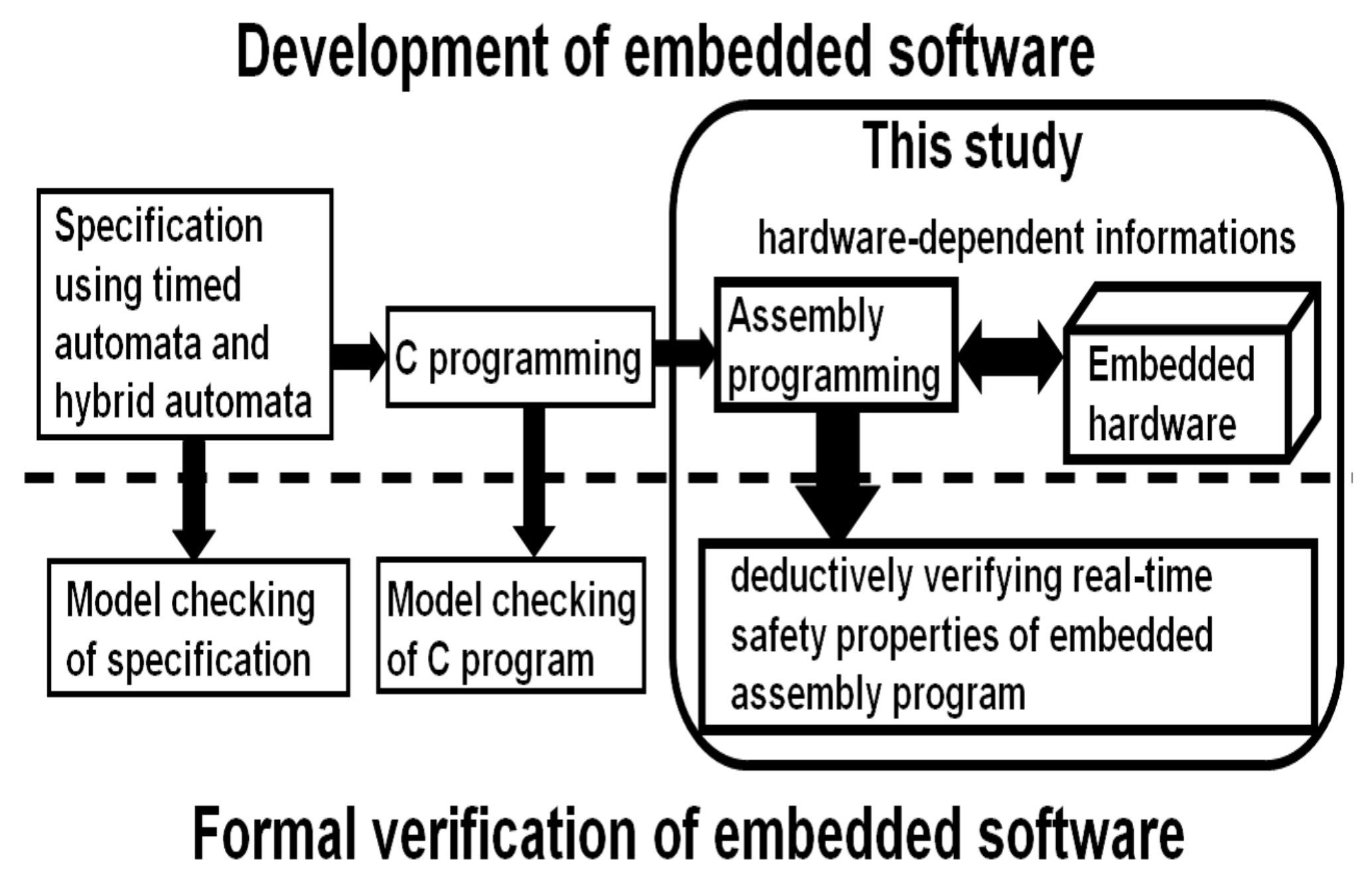
When we develop embedded software, we may first specify it using hybrid automata or timed automata, and then verify it using model checking. Next, we implement it using C program, and verify it using software model checking. In this paper, in order to verify the real-time properties, including hardware-dependent information, we deductively verify the real-time safety properties of an embedded assembly program, as shown in Figure 1.
The embedded software is described in the C language, but the hardware-dependent part is described as an assembly program. Assembly programs are suitable for a prediction of the execution time. Moreover, the syntax of assembly programs are simple, and their analysis is easy. Therefore, in this paper, we verify an assembly program, instead of a C program.
The advantages of verification of assembly programs as pointed out by Schlich [7] are as follows:
- The assembly code is the outcome at the end of the development process. Hence, all errors introduced during the complete development process can possibly be found. These errors include errors not visible in intermediate representations (e.g., re-entrance errors), compiler errors, postcompilation errors (e.g., errors introduced by instrumentation code), and hardware-dependent errors (e.g., stack overflows, arithmetic overflows, interrupt handling errors, and writing reserved registers).
- Assembly language usually has a clean and well-documented semantics. Vendors of microcontrollers provide documentation describing the semantics of the provided assembly constructs. This makes assembly constructs easier to handle than certain C constructs, such as pointer arithmetic or function calls by pointers.
- When model checking assembly code, the model checker does not have to exploit the compiler behavior, hardware-dependent constructs can be handled, and the source code (C code) of the software is not required. Hence, even programs that use libraries not available in the source code can be analyzed.
- Programs consisting of components written in different programming languages can be verified. When model-checking the source code, only single components can be verified and, for each programming language used, a specific model checker has to be utilized.
As shown in Figure 2, we first encode the assembly program into our proposed timed computational model. Secondly, we propose the deductive verification method for real-time safety properties using SMT (Satisfiable Modulo Theories) [8]. Deductive verification method consists of verification rules; one verification rule consists of a temporal formula derived from the premises of first-order formulas. According to [9], we compactly explain a deductive verification method as follows: When we verify whether an assembly program satisfies a safety property, we first encode the assembly program into a timed computational mode. Then, we derive first-order formulas from the timed computational mode, according to a verification rule. Finally, we check validity of the first-order formulas using an SMT solver. If all first-order formulas are valid, the safety property is satisfied.
We propose a timed computational model by assigning the execution time of each instruction to each state.
Using the timed computational model, we can verify the real-time properties of an assembly program. To our knowledge, using a timed computational model that assigns the execution time of each instruction to each state is the first effort in order to verify the real-time properties of an assembly program.
This study is intended for general embedded software, and any RTOS (Real-Time Operating System) is good. We have only adopted H8 as an example In addition, this study is not intended for JAVA programs, as a JAVA program is not an embedded program.
In Section 4, we verify the bounded invariance properties. This example is simple, but we can not verify it by existing methods. Verifying properties related to registers and execution time has been enabled for the first time through our proposed method. We limit this paper to suggesting verification techniques, and more complicated examples are entrusted to future work.
1.2. Related Work
In this section, we present related work regarding assembly program verification and formal verification.
- Execution time of program
- (a)
- As both logical correctness and real-time properties are important in embedded systems, a large number of studies regarding the execution time, such as estimating WCET (Worst Case Execution Time), have been explored by researchers [10]. However, in general, due to the behavior of the components which influence the execution time (such as memory, caches, pipelines, and branch prediction), the predicted execution time from program analysis becomes slightly longer than the real execution time. Therefore, it is important and meaningful to verify whether a formula always holds true within a certain time. As the certain time becomes slightly longer than the real execution time, the formula holds true within a real execution time if it holds true within the certain time. This fact makes verifying liveness properties difficult. In this paper, we verify the real-time properties of an assembly program, based on program analysis.
- Model checking of program
- (a)
- (b)
- Schlich’s [mc]square is famous for the study of the verification of assembly programs [7,14]. The [mc]square system utilizes ELF format execution code information, related C language implementation code, static analysis (CFG) of the target assembly code, specification description using CTL, and a model checker. However, [mc]square cannot verify real-time properties. On the other hand, our study can verify real-time properties using RTLTL. We compute timing information using the execution times of assembly instructions. To the best of our knowledge, our paper is the first study of verifying the timing properties of programs.
- (c)
- The importance of the verification of real-time properties has been pointed out in the model checking of a timed automaton [15]. Campos and Clarke have explored symbolic model checking of discrete real-time systems using RTCTL [16]. All transitions of their timed transition graph happened in one time unit, but the times of timed automata and discrete real-time systems are specified by virtual clocks. However, their model is quite different from our model. A study considering the verification of program execution time has not been carried out, so far, to our knowledge.
- Verification of real-time properties of specification
- (a)
- A. Emerson has explored model checking of discrete real-time systems using RTCTL [17]. On the other hand, Henzinger, Manna, and Pnueli have explored a deductive verification methodology of discrete real-time systems using RTLTL [5]; however, they did not explore real-time verification of real-time programs.
1.3. Theoretical Background of Program Verification Problem
In general, program verification problems are theoretically undecidable [18]. In short, no algorithms exist for program verification. However, this problem is partially decidable. If the answer to the problem is “yes”, the algorithm will eventually halt with a “yes” answer; if the answer is “no”, the algorithm may supply no answer at all. In meaningful cases of real program verification problems, then, the algorithm will eventually halt with a “yes” answer [11,12,13].
On the other hand, in this paper, we give a deductive temporal verification system based on a Hoare-style axiom system for deductively verifying assembly programs. Cook proved a relatively complete Hoare-style axiom system for program verification [19]; in other words, he proved the relative completeness of a Hoare-style axiom system. Furthermore, Manna and Pnueli have proved a relatively complete proof system for proving the validity of temporal properties of reactive programs [20]. Our proof rule is the extension of Manna’s proof system. If we add SMT (Satisfiability Modulo Theories) [8] into our proof rule, we can completely verify assembly programs.
These facts are based on Gödel’s Incompleteness Theorem [21].
2. Computational Model of Embedded Assembly Program
2.1. Embedded Hardware
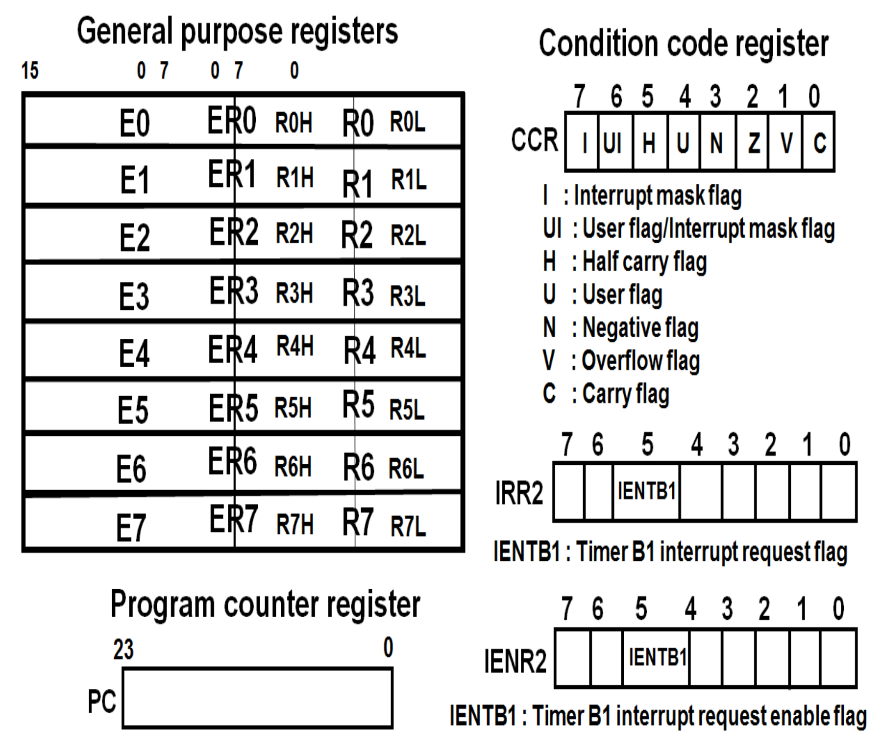
In a H8/3687 processor, all the general purpose registers are 32 bits wide. However, the registers can be treated as the concatenation of two 16-bit registers, such as E0 and R0. The 16-bit registers can also be treated as the concatenation of two 8-bit registers, such as RH0 and RL0. On the other hand, control registers consist of a PC (Program Counter), CCR (Condition Code Register), IRR2 (Interrupt Request Register 2), and IENR2 (Interrupt ENable Register 2). In IRR2, when timer B1 overflows, IENTB1 is set to 1. In IENR2, when IENTB1 is set to 1, the overflow interrupt request of timer B1 is admitted.
2.2. Computational Model
We propose a timed computational model by assigning the execution time of each instruction to each state. The timed computational model is defined as follows:
Definition 1.
(Timed computational model) The timed computational model intended to represent an assembly program is given by the following components:
- 1.
- is a finite set of variables. The set V consists of program variables, a location, the execution time, registers, and a stack.
- 2.
- S is an infinite set of states. Each state assigns to each variable a value.
- 3.
- T is a finite set of transitions. Each transition is a function , which can also be represented by a first-order formula . Here, the variables in V are the present state variables, and the variables in are the next state variables.
- 4.
- Θ is a satisfiable assertion characterizing all the initial states.
- 5.
- is a function assigning to each state the execution time of the natural number. TM is determined by the hardware manual [22], where the execution time of each instruction is described.
- 6.
- is a function assigning to each state an instruction , where is a set of assembly instructions. If no instruction is executed in a state, is omitted in the state.
- 7.
- represents the total of execution time. The total of the execution time can be defined for a point in the execution of the model.
Due to the behavior of the components (such as memory, caches, pipelines, and branch prediction) influencing the execution time, the execution time in this paper becomes slightly longer than the real execution time. However, it is meaningful, from the safety point of view, to verify whether a certain property always holds true within a certain time.
In Section 2.3, we will explain a timed computational model with an example.
2.3. Encoding from Assembly Program to Timed Computational Model
The encoding from a program to a state transition system has a standard hand-operated technique [23]; in particular, we refer to pages 14–16 in [23]. Let V be the set of variables. We think of the variables in V as the present state variables and the variables in as the next state variables. We define a state s to be an interpretation of V, assigning to each variable v a value . Furthermore, we denote a state s to be an interpretation of V as the present state variables, and a state to be an interpretation of as the next state variables. We denote by S the set of all states, and by T the finite set of transitions. Each transition is a function , which is also represented by a first-order formula .
In this paper, we add both the function and a variable time into the set V of variables, where expresses the execution time of the assembly instruction in state s, and a variable expresses the total execution time from the initial state.
Definition 2.
(Deriving Timed computational model) We show how to derive a timed computational model from the first-order formula that represents an assembly program:
- 1.
- The set of states S is the set of all valuations for V.
- 2.
- Let s and be two states. Then, holds true when each is assigned the value s and each is assigned the value .
- 3.
- Θ is defined by an assertion characterizing all the initial states.
- 4.
- TM is determined by the hardware manual [22], in which the execution time of each instruction is described.
- 5.
- is defined by a function assigning to each state an instruction , where is a set of assembly instructions.
- 6.
- is defined by the total execution time from the initial state.
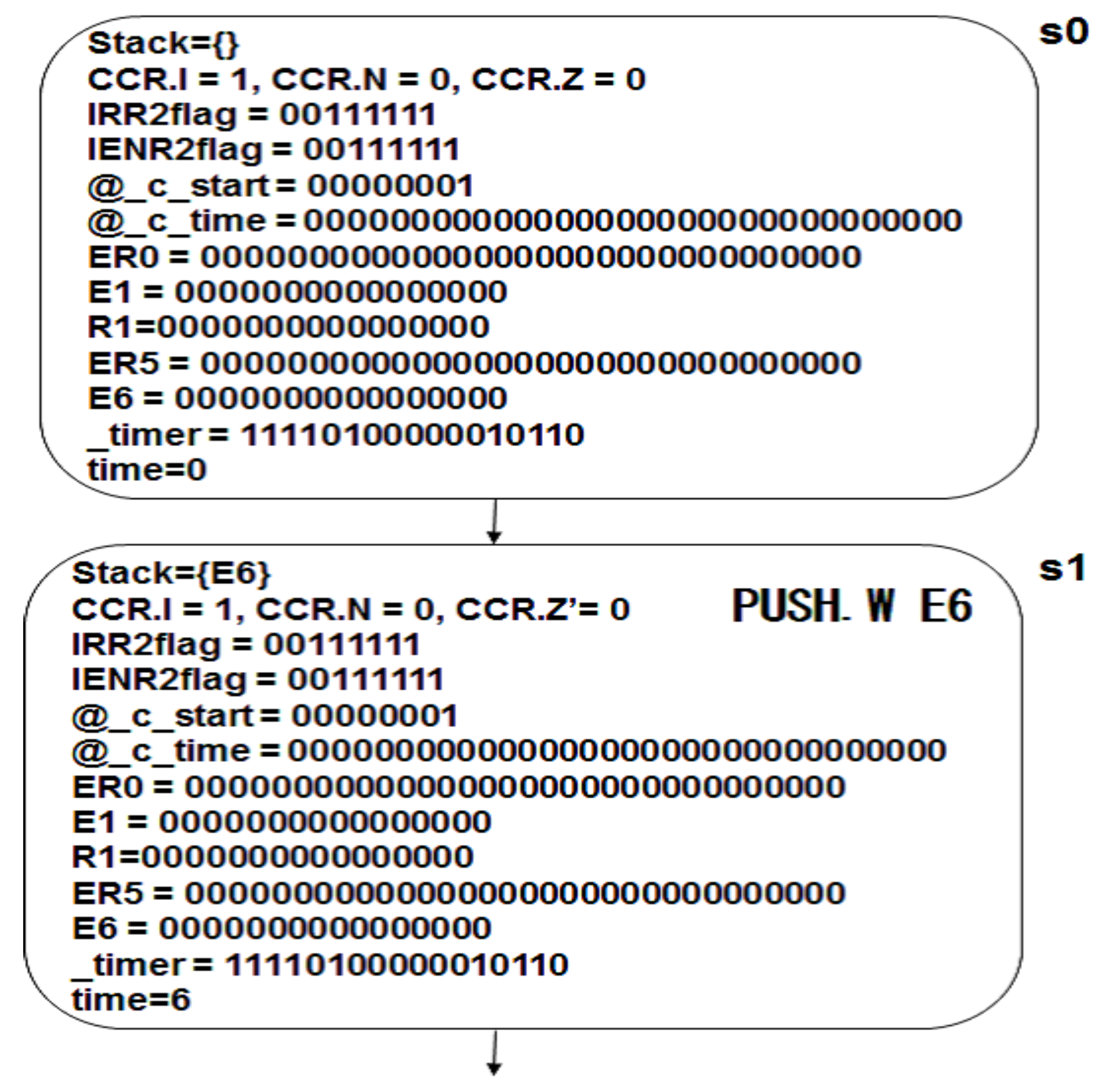
We show a simple example of part of a timed computational model from an assembly program, as follows.
Example 1.
(Example of a timed computational model) An example of a timed computational model generated from assembly program is shown in Figure 4. Each state is defined by the values of variables, registers, individual execution times, stack, and total execution time. As shown in Figure 4, according to [23] and other famous papers, when we derive and specify a state transition system, we omit the ′ representing the next state; in particular, we refer to pages 24–26 in [23].
Here, we define , as in Figure 4, as follows:
- 1.
- .
- 2.
- .For example, we describe and as follows:).).
- 3.
- .For example, we describe , from to , as follows.is represented by a first-order formula :()∧().
- 4.
- We assume .
- 5.
- We define and .
- 6.
- has no label, and has a label (such as PUSH.W E6).
- 7.
- is equal to 6 at .
3. Deductive Verification Using RTLTL
3.1. Real-Time Linear Time Temporal Logic RTLTL
In 1991, Henzinger, Manna, and Pnueli explored RTLTL [5]. RTLTL formulas are constructed from state formulas by Boolean connectives and time-bounded temporal operators.
Definition 3.
(Syntax of RTLTL) We inductively define LTL formulae, as follows:
- 1.
- Each atomic proposition is an LTL formula. In this paper, atomic propositions are propositions such as registers, stack, and execution time. For example, the value of a register is 6.
- 2.
- If p and q are LTL formulae, and are LTL formulae.
- 3.
- If p and q LTL formulae, and are LTL formulae,
where holds at the current step iff p holds at the next moment, and asserts that q does eventually hold and that p will hold everywhere prior to q.
The temporal connective abbreviates and abbreviates .
The temporal connectives ◯, U, ⟡, and □ of LTL are extended by timing constraints, and the temporal connectives , , , and of RTLTL are defined, where denotes the constant of execution time.
Next, we define bounded invariance and bounded response properties. In this paper, we focus on bounded invariance.
- 1.
- Bounded invariance:q, ,
- 2.
- Bounded response:q, .
3.2. Deductive Verification Using RTLTL
In this paper, we extend the deductive verification method explored by Manna and Pnueli [9]. As for the axiom of the deductive verification of temporal logic, the temporal logic formula is derived by premises to consist of predicate logic formulas [9]. This is the most important work of Amir Pnueli, which won the ACM A.M. Turing Award in 1996 [24]. This study expands on A. Pnueli’s study by adding execution time, and develops the axiom of deduction verification using RTLTL.
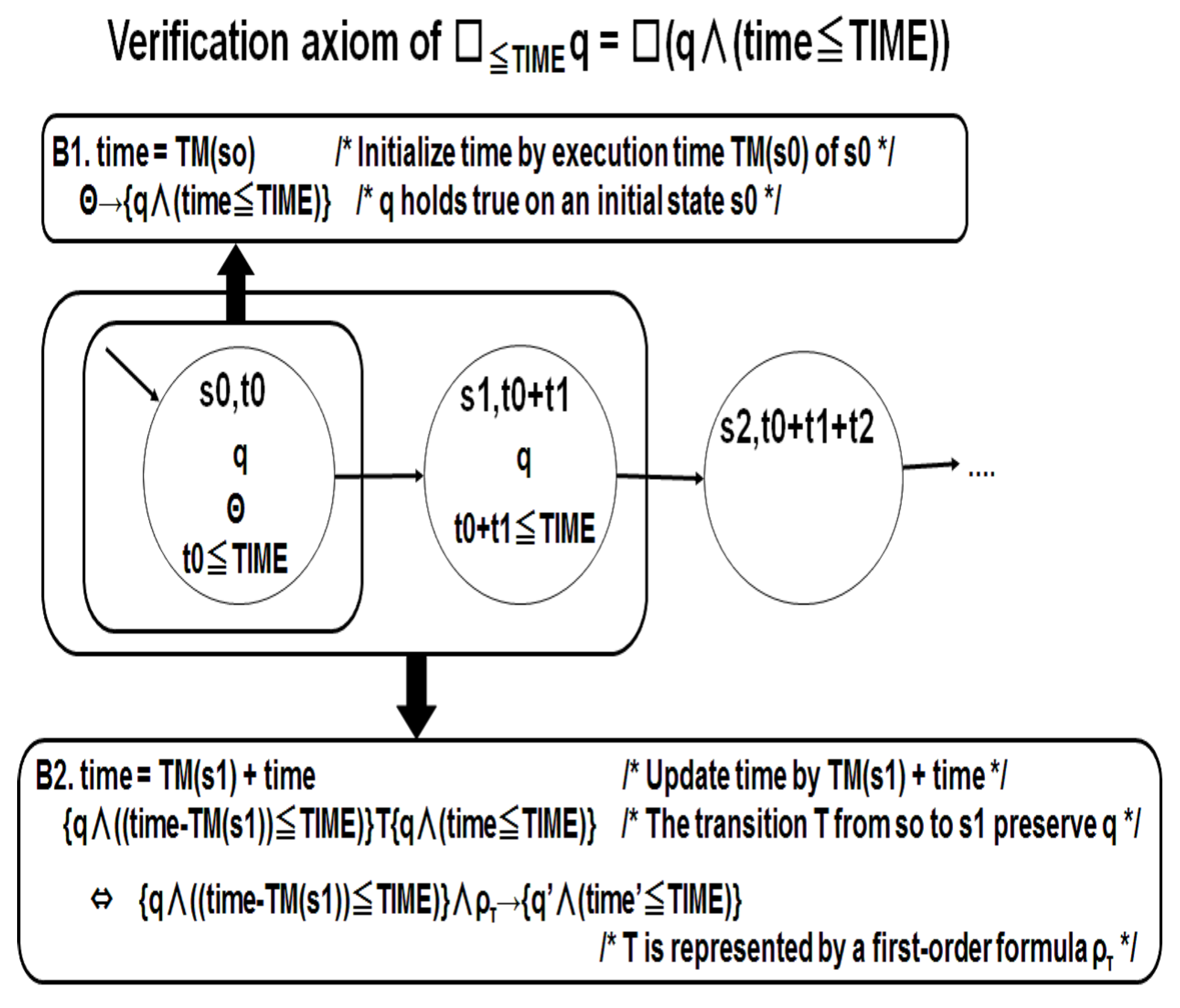
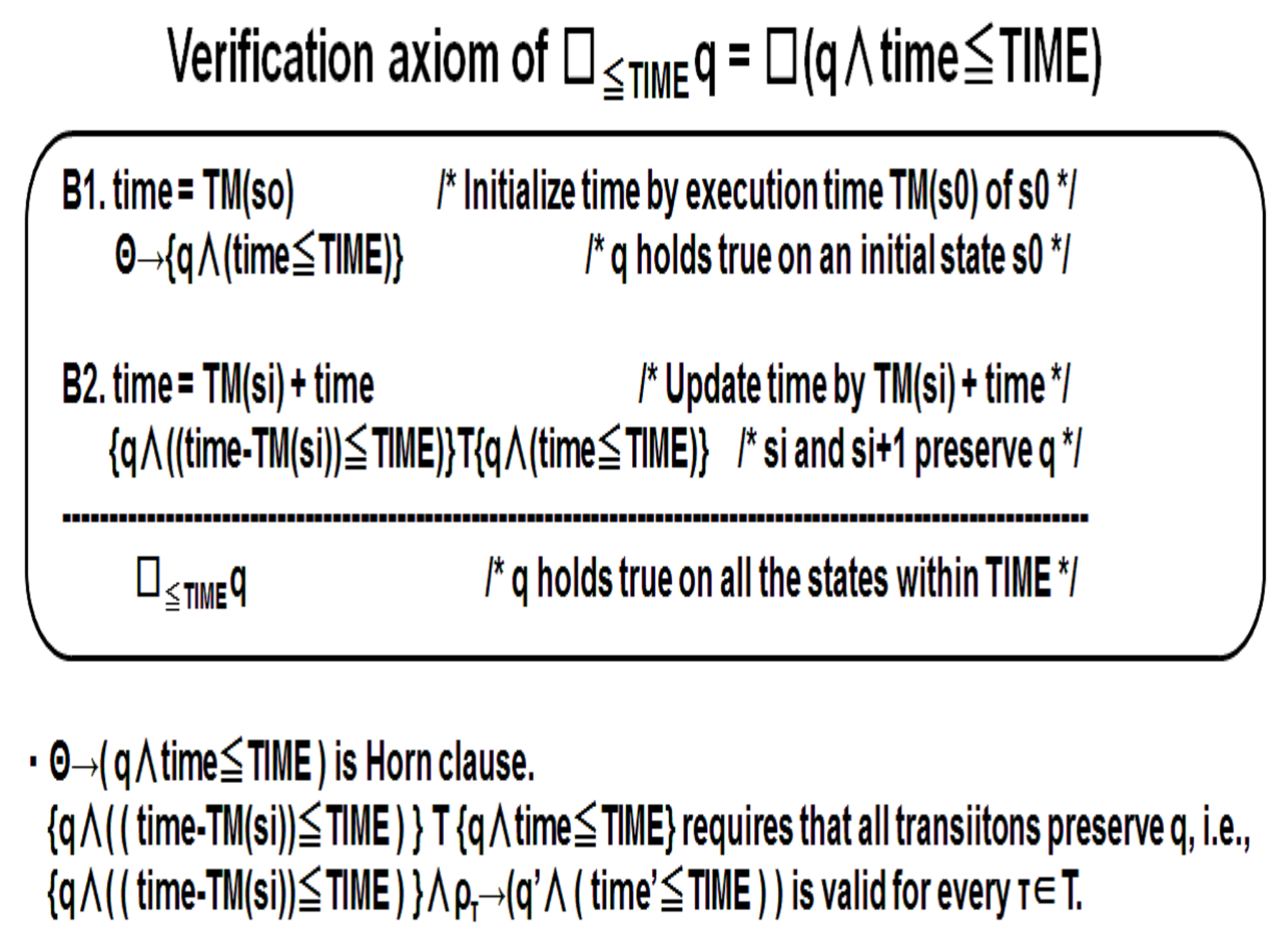
In this paper, as shown in Figure 5, we construct a part of our verification axiom q as over a timed computational model. In Figure 5, we introduce a variable to measure execution time.
In Figure 6, if Premises B1 and B2 are valid, q is obviously valid. Therefore, this axiom is sound. Furthermore, our timed transition model is the same as Henzinger’s timed transition system [5] when the minimal delay is equal to the maximal delay. Therefore, we can prove that our verification axiom is relatively complete by Henzinger’s proof technique [5].
When we verify an assembly program using our verification axiom, a set of first-order formulae are constructed. We can verify whether each formula is valid or not using an SMT solver [3].
Premise B1 requires that the time is set to at an initial state and the initial condition implies . Premise B2 requires that the time is set to and all transitions preserve .
4. Experiments of Deductive Verification of Real-Time Properties
We try to deductively verify embedded an assembly program. We used the Linetrace program written, for the Wheel-type robot nuvo WHEEL controlled by a H8/3687 microcontroller [4]. The Linetrace program acquires values from a sensor, and operates a robot from the values. The robot has three sensors and a motor: the sensors can distinguish black from white, and output either 0 or 1 by color; the motor is controlled by PID control. When a timer overflow interrupt of timer B1 occurs, H8/3687 acquires the value from a sensor, and sets the new current targeted value from the value. When a timer overflow interrupt of timer V occurs, H8/3687 performs PID control from the current targeted value and the current value, and outputs the value in the motor.
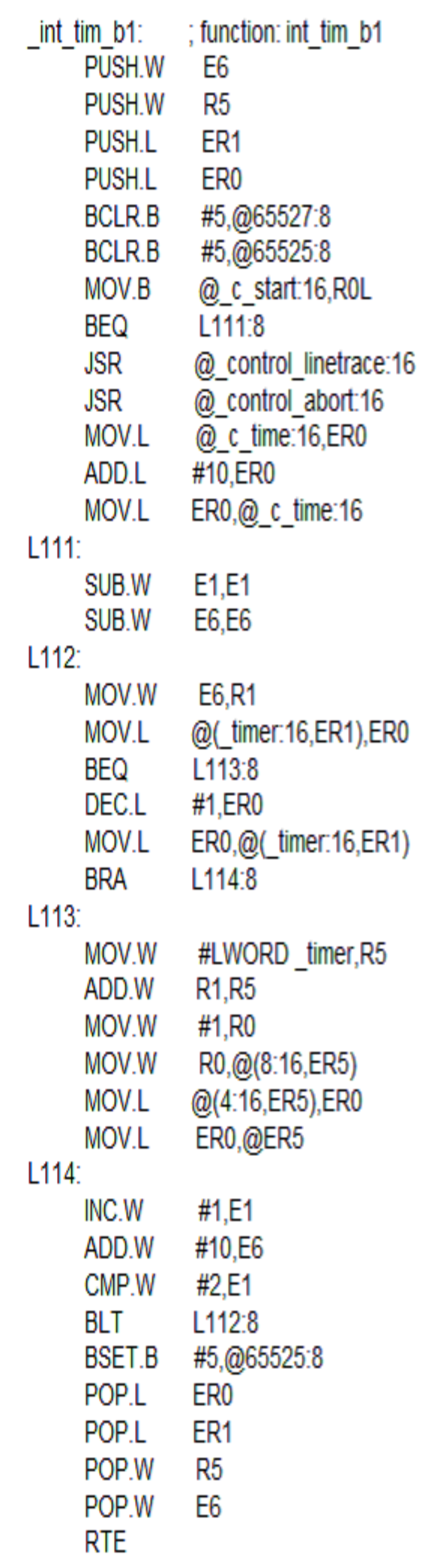
In this section, we verify a timer interrupt function . If is executed, it acquires the value of the sensor and decides the current targeted value. It returns to processing before the interrupt.
An assembly program of a timer interrupt function is shown in Figure 7.
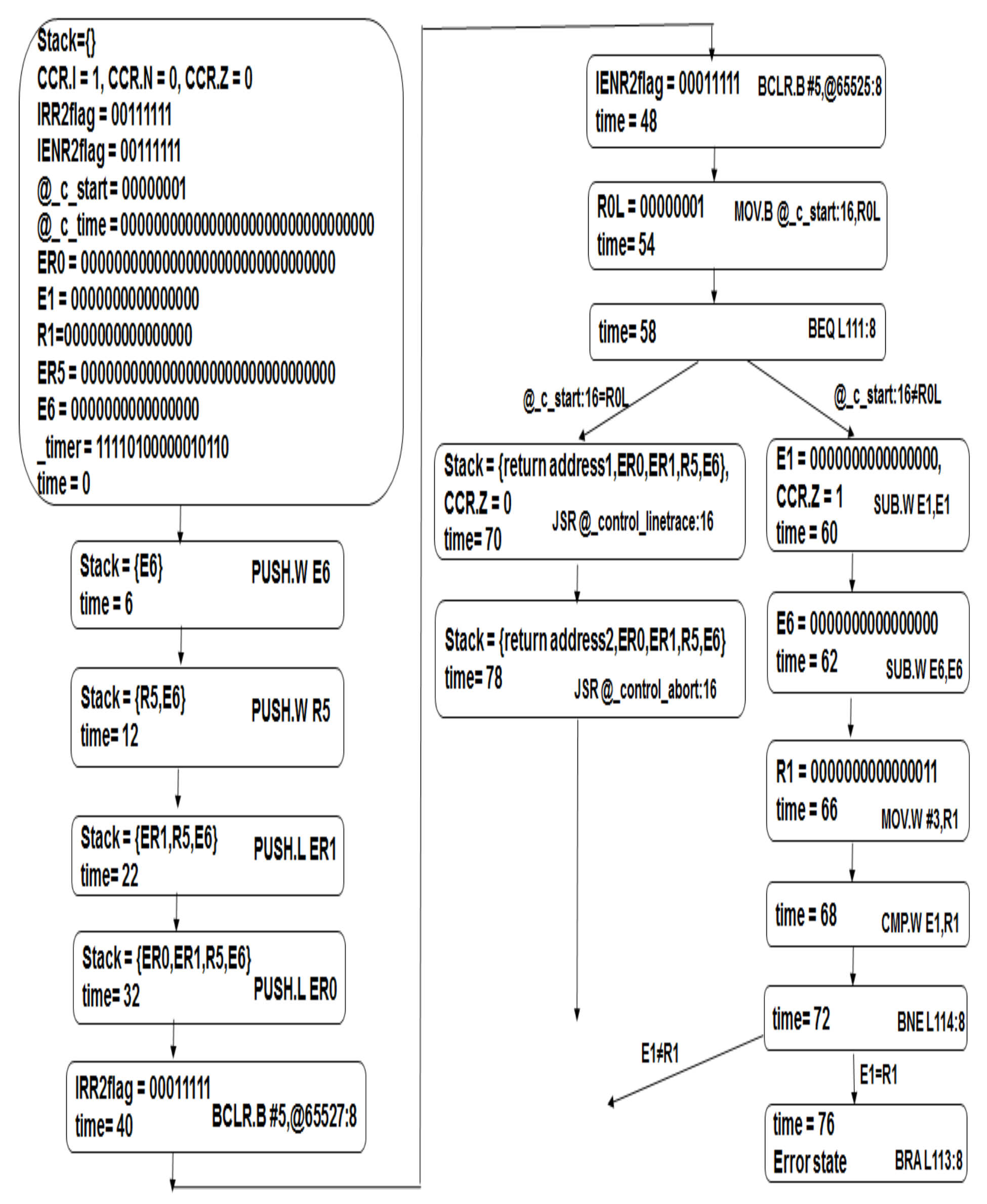
We show a timed computational model of a timer interrupt function in Figure 8. In Figure 8, we describe only the values that have changed from the previous state in the current state.
- First, a state is defined by the values of stacks, flags, variables, timers, and execution times. Execution time is the number of states, and one state is 0.05 microseconds.
- Next, we verify whether holds true. When holds true, we also check whether the program has reached an error state ( and ).The statement means that, within execution time 75, the registers E1 and R1 are equal. As existing tools can not compute the execution time, we can not verify using existing tools [7].
- Next, we verify whether holds true, as follows:
- (a)
- B1. , .Initially, let , where measures the total execution time.is as follows:00000000000000000000000000000000.Let = . As and hold true, is valid. We check whether is valid using the SAT/SMT solver Princess [3].
- (b)
- B2. , :where is equal to .
- →We checked whether the above first-order formula is valid using the SAT/SMT solver Princess [3], as shown in the Appendix A. The above first-order formula is valid.
- →We checked whether the above first-order formula is valid using SAT/SMT solver Princess [3]. The above first-order formula is valid.
- →We checked whether the above first-order formula is valid using the SAT/SMT solver Princess [3]. The above first-order formula is valid.
Finally, when holds true, the function does not arrive at an error state, in which case and hold true.
Finally, holds true.
5. Conclusions and Future Work
We have proposed a deductive verification method in order to verify the real-time safety properties of an embedded assembly program, in the following manner:
- First, we constructed a timed computational model including the execution time from the assembly program. We could specify an infinite state transition system including the execution time by the timed computational model.
- Next, we developed a verification axiom of q. We verified whether a timed computational model satisfies RTLTL (Real-Time Linear Temporal Logic) formulas by deductive verification.
- We also implemented our proposed axiom in the theorem prover Princess [3].
- Finally, we demonstrated experiments with real examples, such as the Linetrace program written for the Wheel-type robot nuvo WHEEL controlled by the H8/3687 microcontroller [4]. This robot is very old, but it has the important features of embedded software.
Using our proposed methods, we were able to achieve verification of the real-time safety properties such as q of an embedded assembly program. In addition, we have demonstrated experiments with real examples. It is worth noting that deductive verification is tedious work.
We are now working on the model-checking of real-time safety and liveness properties of assembly program [25]. Furthermore, we are working on a CEGAR-based model checking method [26], based on the work of Rybalchenko [27]. Our recent results [25,26] are fully automatic verification methods without manual verifications, freeing you from tedious work. However, even if we can verify some program by our proposed method in this paper, we can not verify the program by our recent results [25,26]. The best way would be to combine these two approaches.
Acknowledgments
This work was supported in part by JSPS/MEXT Grant-in-Aid for Scientific Research Numbers 15K00093.
Conflicts of Interest
The authors declare no conflicts of interest.
Appendix A
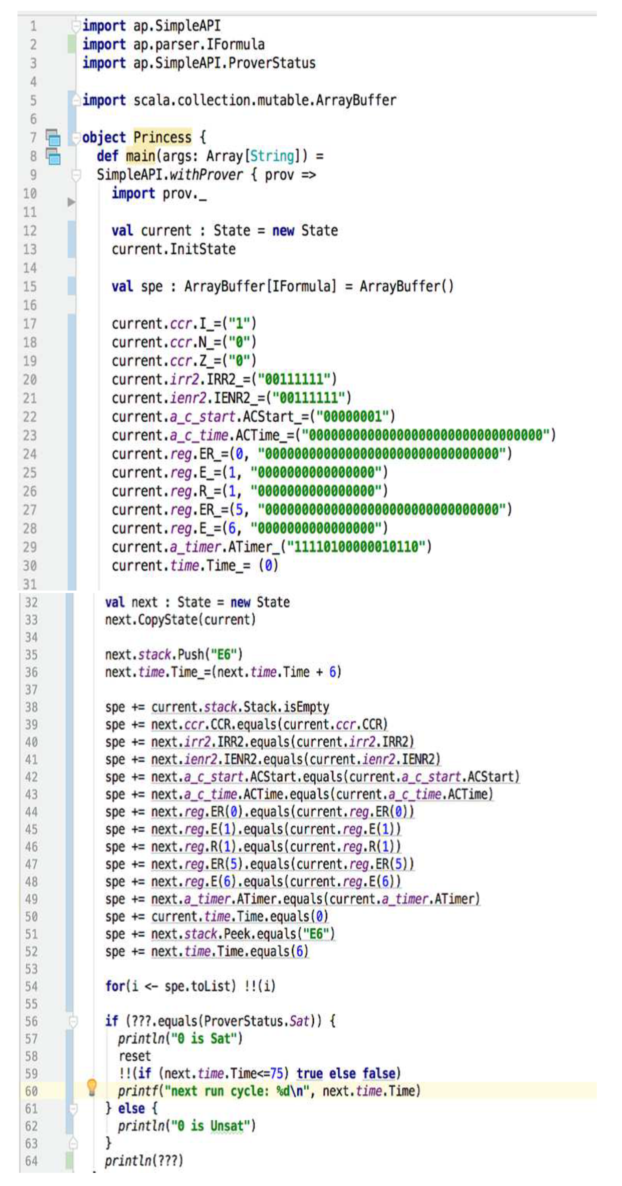
We show the method for checking whether the first-order formula mentioned above is valid using the SAT/SMT solver Princess [3], as follows.
We input the program codes shown in Figure A1 into Princess.
Figure A1.
Example of program codes input into Princess.

From lines 17–30, the current state is specified. From lines 38–52, the state transition is specified.
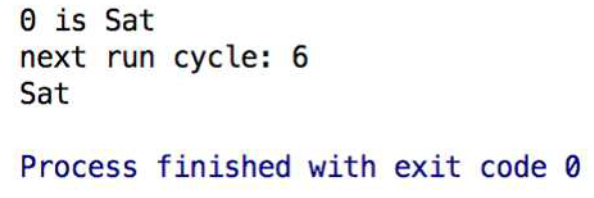
Following this, Princess proves the formula and outputs the verification result shown in Figure A2. Here, Sat is the output. If the quantifier-free formula, such as , is satisfiable, the formula is valid. Therefore, the first-order formula is valid.
Figure A2.
Princess output of the verification result.

References
- Jhala, R. Majumdar: Software model checking. ACM Comput. Surv. (CSUR) 2009, 41, 21. [Google Scholar] [CrossRef]
- Yamane, S. Deductively verifying embedded software in the era of artificial intelligence = machine learning + software science. In Proceedings of the IEEE 6th Global Conference on Consumer Electronics (GCCE), Nagoya, Japan, 24–27 October 2017; pp. 1–4. [Google Scholar]
- Rummer, P. Available online: http://www.philipp.ruemmer.org/princess.shtml (accessed on 12 October 2019).
- ZMP. Available online: https://robot.watch.impress.co.jp/cda/news/2006/07/12/81.html (accessed on 12 October 2019).
- Henzinger, T.A.; Manna, Z.; Pnueli, A. Temporal Proof Methodologies for Timed Transition Systems. Inf. Comput. 1994, 112, 273–337. [Google Scholar] [CrossRef]
- Yamane, S.; Konoshita, R.; Kato, T. Model checking of embedded assembly program based on simulation. IEICE Trans. Inf. Syst. 2017, E100-D, 1819–1826. [Google Scholar] [CrossRef]
- Schlich, B. Model checking of software for microcontrollers. ACM Trans. Embedded Comput. Syst. 2010, 9, 36. [Google Scholar] [CrossRef]
- Bjorner, N.; McMillan, K.L.; Rybalchenko, A. Program Verification as Satisfiability Modulo Theories. In Proceedings of the 10th International Workshop on Satisfiability Modulo Theories(SMT 2012), Manchester, UK, 30 June–1 July 2012; pp. 3–11. [Google Scholar]
- Manna, Z.; Pnueli, A. Temporal Verification of Reactive Systems: Safety; Springer: Berlin/Heidelberg, Germany, 1994. [Google Scholar]
- Wilhelm, R.; Engblom, J.; Ermedahl, A.; Holsti, N.; Thesing, S.; Whalley, D.; Bernat, G.; Ferdinand, C.; Heckmann, R.; Mitra, T.; et al. The worst-case execution-time problem-overview of methods and survey of tools. ACM Trans. Embed. Comput. Syst. (TECS) 2008, 7, 36. [Google Scholar] [CrossRef]
- Ball, T.; Majumdar, R.; Millstein, T.D.; Rajamani, S.K. Automatic Predicate Abstraction of C Programs. In Proceedings of the ACM SIGPLAN 2001 Conference on Programming Language Design and Implementation (PLDI ’01), Snowbird, UT, USA, 20–22 June 2001; pp. 203–213. [Google Scholar]
- Henzinger, T.A.; Jhala, R.; Majumdar, R.; Sutre, G. Lazy abstraction. In Proceedings of the 29th ACM SIGPLAN-SIGACT Symposium on Principles of Programming Languages (POPL ’02), Portland, OR, USA, 16–18 January 2002; pp. 58–70. [Google Scholar]
- Chaki, S.; Clarke, E.M.; Groce, A.; Jha, S.; Veith, H. Modular Verification of Software Components in C. IEEE Trans. Softw. Eng. 2004, 30, 388–402. [Google Scholar] [CrossRef]
- Noll, T.; Schlich, B. Delayed Nondeterminism in Model Checking Embedded Systems Assembly Code. In LNCS; Springer: Berlin, Germany, 2008; Volume 4899, pp. 185–201. [Google Scholar]
- Alur, R.; Dill, D.L. A Theory of Timed Automata. Theor. Comput. Sci. 1994, 126, 183–235. [Google Scholar] [CrossRef]
- Campos, S.V.A.; Clarke, E.M.; Marrero, W.R.; Minea, M.; Hiraishi, H. Temporal Verification of Real-Time Systems. IEICE Trans. 1995, 78-D, 96–801. [Google Scholar]
- Emerson, E.A.; Mok, A.K.; Sistla, A.P.; Srinivasan, J. Quantitative Temporal Reasoning. In LNCS; Springer: Berlin, Germany, 1990; Volume 531, pp. 136–145. [Google Scholar]
- Turing, A.M. On computable numbers, with an application to the Entscheidungsproblem. Proc. Lond. Math. Soc. 1937, 116–155. [Google Scholar] [CrossRef]
- Cook, S.A. Soundness and completeness of an axiom system for program verification. SIAM J. Comput. 1978, 7, 70–90. [Google Scholar] [CrossRef]
- Manna, Z.; Pnueli, A. Completing the Temporal Picture. Theor. Comput. Sci. 1991, 83, 91–130. [Google Scholar] [CrossRef]
- Gödel, K. Uber formal unentscheidbare SAtze der Principia Mathematica und verwandter Systeme, I. Monatshefte Fur Math. Und Phys. 1931, 38, 173–198. [Google Scholar] [CrossRef]
- Renesas: H83687 Group Hardware Manual. Available online: https://www.renesas.com/jp/ja/products/microcontrollers-microprocessors/h8/h8300h-tiny/h83687-h83687n.html (accessed on 12 October 2019).
- Clarke, E.M.; Grumberg, O.; Peled, D. Model Checking; MIT Press: Cambridge, MA, USA, 1999. [Google Scholar]
- Pnueli, A. The Temporal Logic of Programs. In Proceedings of the 18th Annual Symposium on Foundations of Computer Science (FOCS 1977), Providence, RI, USA, 31 October–1 November 1977; pp. 46–57. [Google Scholar]
- Wu, Y.; Yamane, S. Model Checking of Embedded Systems Using RTCTL While Generating Timed Kripke Structure. In Proceedings of the 2018 IEEE 42nd Annual Computer Software and Applications Conference (COMPSAC), Tokyo, Japan, 23–27 July 2018; p. 257. [Google Scholar]
- Kamide, H.; Uemura, K.; Yamane, S. Model Check of Real-time Property of Embedded Assembly Program Using CEGAR. In Proceedings of the 2018 IEEE 42nd Annual Computer Software and Applications Conference (COMPSAC), Tokyo, Japan, 23–27 July 2018; pp. 799–800. [Google Scholar]
- Gupta, A.; Popeea, C.; Rybalchenko, A. Predicate abstraction and refinement for verifying multi-threaded programs. In Proceedings of the Proceedings of the 38th annual ACM SIGPLAN-SIGACT symposium on Principles of programming languages (POPL ’11), Austin, TX, USA, 26–28 January 2011; pp. 331–344. [Google Scholar]
Figure 1.
Overview of this study.

Figure 2.
Outline of this study.

Figure 3.
Register set of a H8/3687 processor.

Figure 4.
Example of part of a timed computational model from an assembly program.

Figure 5.
Part of the verification axiom of q.

Figure 6.
Verification axiom of q.

Figure 7.
Assembly program of a timer interrupt function .

Figure 8.
A timed computational model of .

© 2019 by the author. Licensee MDPI, Basel, Switzerland. This article is an open access article distributed under the terms and conditions of the Creative Commons Attribution (CC BY) license (http://creativecommons.org/licenses/by/4.0/).
Share and Cite
MDPI and ACS Style
Yamane, S. Deductive Verification Method of Real-Time Safety Properties for Embedded Assembly Programs. Electronics 2019, 8, 1163. https://doi.org/10.3390/electronics8101163
AMA Style
Yamane S. Deductive Verification Method of Real-Time Safety Properties for Embedded Assembly Programs. Electronics. 2019; 8(10):1163. https://doi.org/10.3390/electronics8101163
Chicago/Turabian StyleYamane, Satoshi. 2019. "Deductive Verification Method of Real-Time Safety Properties for Embedded Assembly Programs" Electronics 8, no. 10: 1163. https://doi.org/10.3390/electronics8101163
Note that from the first issue of 2016, this journal uses article numbers instead of page numbers. See further details here.