A Mixed Deep Recurrent Neural Network for MEMS Gyroscope Noise Suppressing

Abstract

Currently, positioning, navigation, and timing information is becoming more and more vital for both civil and military applications. Integration of the global navigation satellite system and /inertial navigation system is the most popular solution for various carriers or vehicle positioning. As is well-known, the global navigation satellite system positioning accuracy will degrade in signal challenging environments. Under this condition, the integration system will fade to a standalone inertial navigation system outputting navigation solutions. However, without outer aiding, positioning errors of the inertial navigation system diverge quickly due to the noise contained in the raw data of the inertial measurement unit. In particular, the micromechanics system inertial measurement unit experiences more complex errors due to the manufacturing technology. To improve the navigation accuracy of inertial navigation systems, one effective approach is to model the raw signal noise and suppress it. Commonly, an inertial measurement unit is composed of three gyroscopes and three accelerometers, among them, the gyroscopes play an important role in the accuracy of the inertial navigation system’s navigation solutions. Motivated by this problem, in this paper, an advanced deep recurrent neural network was employed and evaluated in noise modeling of a micromechanics system gyroscope. Specifically, a deep long short term memory recurrent neural network and a deep gated recurrent unit–recurrent neural network were combined together to construct a two-layer recurrent neural network for noise modeling. In this method, the gyroscope data were treated as a time series, and a real dataset from a micromechanics system inertial measurement unit was employed in the experiments. The results showed that, compared to the two-layer long short term memory, the three-axis attitude errors of the mixed long short term memory–gated recurrent unit decreased by 7.8%, 20.0%, and 5.1%. When compared with the two-layer gated recurrent unit, the proposed method showed 15.9%, 14.3%, and 10.5% improvement. These results supported a positive conclusion on the performance of designed method, specifically, the mixed deep recurrent neural networks outperformed than the two-layer gated recurrent unit and the two-layer long short term memory recurrent neural networks.

1. Introduction

With the booming of location based services (LBS), positioning, navigation, and timing (PNT) information is more essential than at any time in human history, since more and more smart devices relies on PNT information [1]. Currently, the global navigation satellite system (GNSS) has been the most widely used PNT information provider and generator, due to its easy access, low cost, and high accuracy. Broadly speaking, the GNSS refers to all satellite based navigation systems, including global and regional systems. Among them, the USA Global Positioning System (GPS), China BeiDou Navigation System (BDS), Europe Galileo Satellite Navigation System (Galileo), and the Russia Global Navigation Satellite System (GLONASS) are capable of global coverage, and other regional systems, for instance Japan’s Quasi-Zenith Satellite System (QZSS) and the Indian Regional Navigation Satellite System (IRNSS), offer an augmentation of GPS for performance enhancement in specific regions [1,2,3]. Generally, their working principles are similar, and the details are as follows: (1) firstly, the satellites in orbit broadcast navigation signals to the Earth, and the signals are modulated with information of the satellites’ orbit description parameters and some other information; (2) secondly, the user receives the broadcast signals and de-modulates the information, which can be employed to obtain the distance between the user and satellites; (3) thirdly, with at least four satellites in view, the PNT information can be determined precisely using a least-square algorithm or Kalman filter [1,2,3,4,5]. The advantages of GNSS are summarized as: (1) GNSS is able to provide precise navigation solutions at low cost, since a handheld chip receiver is cheap and sufficient for common applications; (2) GNSS is an all-weather navigation system covering the earth, and its positioning accuracy does not diverge over time. However, apart from these advantages, it also has some drawbacks limiting its further application: (1) firstly, the satellites are far away from the Earth, thus, the signals are pretty weak when they reach the Earth; (2) secondly, GNSS civil signal structure is open to the public, which makes GNSS extremely sensitive to interference and spoofing; (3) thirdly, temporary signal blockages or obstruction can also render the GNSS receiver unavailable to the satellite signals [6,7,8,9,10]. A standalone GNSS is not sufficient to provide seamless PNT information, thus they are commonly integrated with an inertial navigation system (INS) to provide ubiquitous navigation solutions [6,7,8,9,10]. While the GNSS is unavailable, the INS outputs the positioning information for users during the signal outage.

INS is another navigation system capable of providing position, velocity, and attitude information. An INS is constructed through processing raw data or signals from the inertial measurement unit (IMU). Commonly, an IMU consists of three accelerometers and gyroscopes. Positioning errors divergence is usually caused by the noise contained in raw signals from the gyroscopes and accelerometers. Recently, due to the low cost and small size of the advanced micro-mechanics system (MEMS) manufacturing technology, the MEMS IMU has become more popular in the community for developing low cost and highly accurate GNSS/INS integrated navigation systems. However, as the MEMS IMU experiences more complex errors and noises, it is of great significance to develop a noise modeling method for the MEMS IMU [11,12,13,14,15,16,17,18,19], especially for improving positioning accuracy during GNSS signal outages.

In INS, gyroscopes play an important role in INS positioning accuracy, thus, past works have mostly focused on modeling and suppressing the noise of the MEMS gyroscopes [11,12,13,14,15,16,17,18,19]. Various methods have been proposed and evaluated in MEMS gyroscope noise analysis and modeling; and basically, the methods can be classified into two approaches: statistical method and artificial intelligence method. In the statistical methods, Allan Variance (AV) and Auto Regressive Moving Average (ARMA) are the most popular. AV was first employed in MEMS IMU noise analysis and errors description in 2004 [19]. In the AV method, five basic parameters are introduced to describe the gyroscopes’ and accelerometers’ noise, and the parameters are termed as: quantization noise, angle random walk, bias instability, rate random walk, and rate ramp [19,20,21,22,23,24]. ARMA is another method for MEMS gyroscope noise modeling and compensation, in which the raw data are treated as time series. Variants of ARMA have also been proposed to furtherly improve the performance [25,26,27,28,29]. Moreover, artificial intelligence methods, such as support vector machines (SVM) and neural networks (NN), have also been employed in this application to obtain better de-noising performance [30,31,32]. The results demonstrate the effectiveness of these methods in this application. However, both of the two solutions have some drawbacks, the statistical method usually has fixed parameters, which are not sufficient for certain applications; the artificial methods usually have limited ability to learn the model, due to their simple structures.

Recently, Deep Learning (DL) has gained a boom and performed excellently in various applications including image processing, Nature Language Processing (NLP) and sequential signal processing [30,31,32,33,34,35,36,37]. In aspects of time series processing, a recurrent neural network (RNN) was always the most feasible selection [30,31,32,33,34,35,36,37]. A common RNN was not sufficient, thus, variants of RNN were proposed for enhancing the performance. Among the variants, Long Short Term Memory (LSTM) and the Gated Recurrent Unit (GRU) were most popular. LSTM-RNN and GRU-RNN both obtained excellent performance in NLP [30,31,32,33,34,35,36,37]. In addition, in our previous paper, LSTM was employed and compared in MEMS gyroscope de-noising [8]. With fixed or identical length of training examples, LSTM had better training accuracy, but GRU had better convergence efficiency for its unique design [8]. Commonly, GRU was designed with less parameters than LSTM, and this made GRU coverage faster and quickly than LSTM in training procedures.

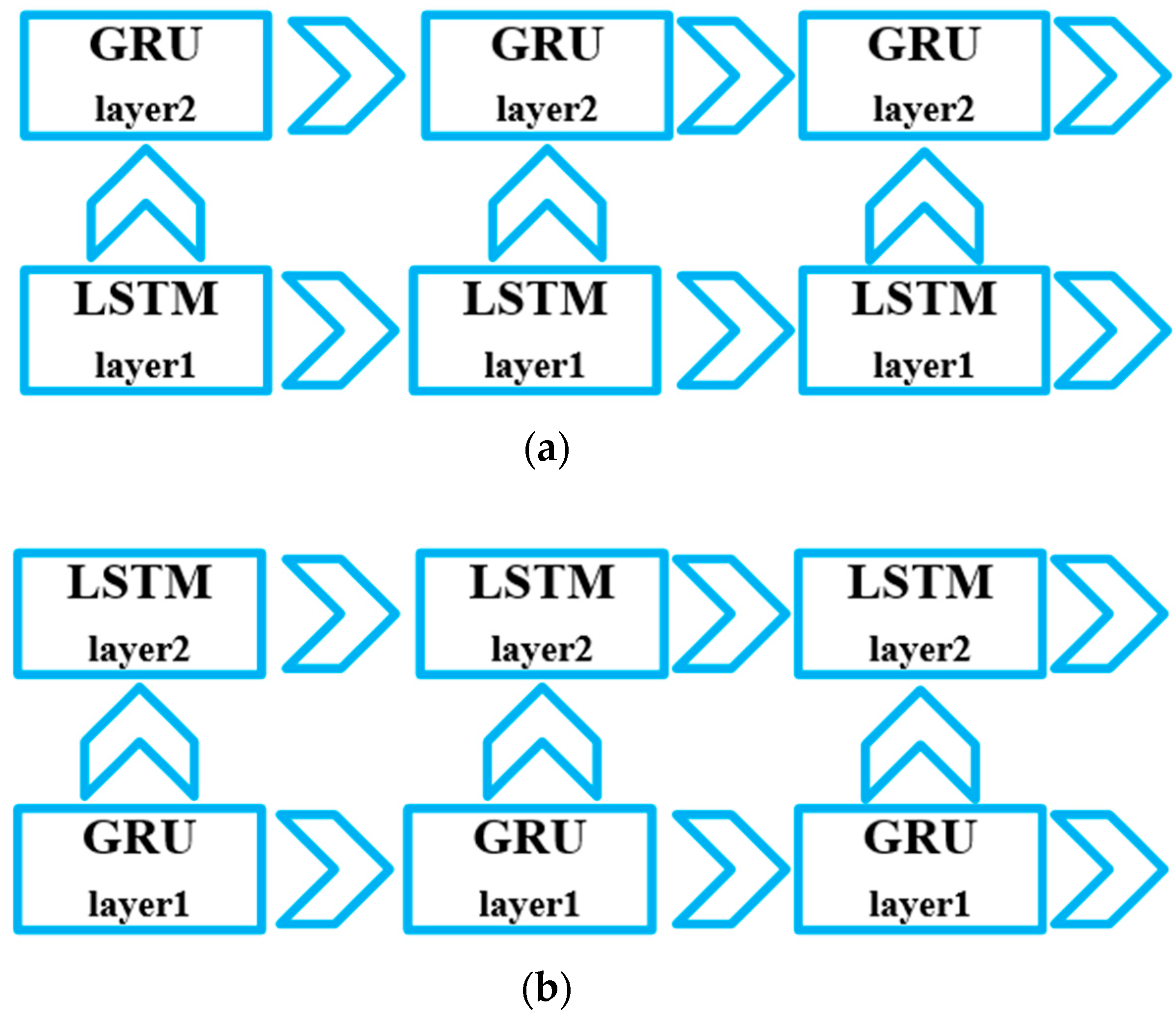
Inspired by the multi-layer RNN design scheme, a new architecture combing LSTM and GRU together was explored for MEMS gyroscope noise modeling in the paper. As aforementioned, since the GRU and LSTM had different characteristics, it was meaningful to explore the mixed LSTM and GRU in this application. Specifically, in this paper, two multi-layer RNNs with different architectures (LSTM–GRU: first layer, LSTM; second layer, GRU. GRU–LSTM: first layer, GRU; second layer: LSTM) of LSTM and GRU combination were investigated.

In this method, a GRU unit was substituted by a LSTM unit in a two layer GRU-RNN, thus, the method was expected to combine the advantages from the LSTM and GRU. An MEMS IMU dataset was collected to evaluate the proposed method, and compare the results with a common multi–layer GRU-RNN and multi-layer LSTM-RNN. Firstly, LSTM–GRU and GRU–LSTM were compared to select the proper structure for this application. Secondly, the new method was compared with a multi-layer LSTM-RNN and multi-layer GRU-RNN for a more specific analysis of performance. Finally, the standard deviation of the filtered signals and the attitude errors were presented. We thought the contributions of this paper could be summarized as:

(1)

It was the first time a mixed LSTM and GRU method has been applied to MEMS gyroscope noise modeling, which might be an inspiration for applying DL in MEMS IMU de-noising.

(2)

It was a bright idea to develop a mixed multi-layer RNN; detailed analysis of the multi-layer LSTM, multi-layer GRU, LSTM–GRU, and GRU–LSTM were presented and compared, which could provide valid reference while selecting proper methods for MEMS gyroscope noise modeling.

The remainder of this paper is organized as follows: Section 2 describes the structures and the equations of the employed RNN, including the LSTM unit, GRU unit, and the mixed LSTM and GRU. Section 3 introduces the experiments, results, and analysis of these methods. The remaining sections are the discussion, conclusion, acknowledgements, and the references.

2. Methods

In this section, the basic structure and detailed mathematical equations are listed. This section is divided into four subsections. Section 2.1 is the basic introduction of the LSTM unit, Section 2.2 is about the GRU, Section 2.3 presents the combination of LSTM and GRU.

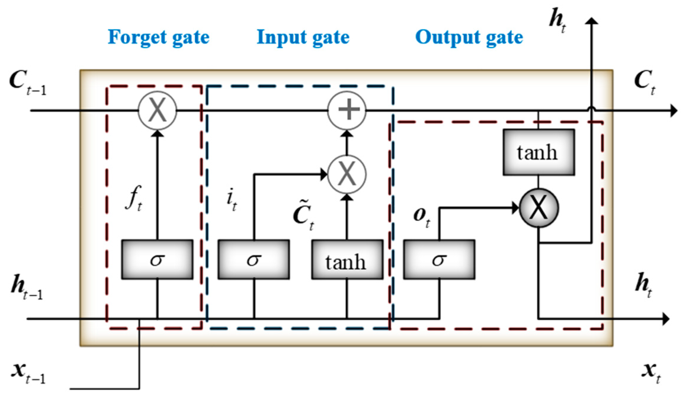
2.1. Long Short Term Memory (LSTM)

As is well-known, LSTM is built using a unique ‘gate’ structure. Figure 1 shows the basic components of a LSTM. ‘Forget,’ ‘Input,’ and ‘Output’ gates work cooperatively to accomplish the function of a LSTM unit and control the information flow. As presented in Figure 1, from left to the right, the first component is the ‘forget’ gate, and a sigmoid function $\sigma (\cdot )$ is employed in this gate to decide what information will be memorized from the previous state cell. The details of this procedure are listed as the following Equation (1).

$${\mathit{f}}_t=\sigma \left({\mathit{W}}_f\cdot \left[{\mathit{h}}_{t-1},{\mathit{x}}_t\right]+{\mathit{b}}_f\right)$$

(1)

where, $\sigma (\cdot )$ is the sigmoid function, ${\mathit{W}}_f$ and ${\mathit{b}}_f$ are the parameters that will be determined after training, ${\mathit{h}}_{t-1}$ is the hidden state at time epoch $t-1$, and ${\mathit{x}}_t$ is the input vector at time epoch $t$. Vector ${\mathit{f}}_t$ is the output of the sigmoid function.

The inputs of the function are the hidden state from the previous LSTM unit and input vector. Outputs of the functions are values ranging from 0 to 1, which correspond to each number in the cell state from the previous LSTM unit. The values represent the forgetting degree of each number in the previous cell state ${\mathit{C}}_{t-1}$. A value of ‘1’ means ‘completely keeping this,’ and, oppositely, a value of ‘0’ means ‘completely forgetting or excluding.

After the “forget“ gate, the following is the ‘input’ gate, which controls the input and decides what part of the new information will be stored in the current cell state. The procedure is operated using the following two functions, Equations (2) and (3). Equation (2) is a sigmoid function similar to Equation (1). This function is employed to decide the updating degree of each number in the input vector. Equation (3) is a tanh layer, which outputs a new cell state ${\tilde{\mathit{C}}}_t$. Later, the new, hidden ${\tilde{\mathit{C}}}_t$ is multiplied with the vector $i$, and then added to the current cell state.

$${\mathit{i}}_t=\sigma \left({\mathit{W}}_i\cdot \left[{\mathit{h}}_{t-1},{\mathit{x}}_t\right]+{\mathit{b}}_i\right)$$

(2)

$${\tilde{\mathit{C}}}_t=\tanh \left({\mathit{W}}_C\cdot \left[{\mathit{h}}_{t-1},{\mathit{x}}_t\right]+{\mathit{b}}_C\right)$$

(3)

where $\sigma (\cdot )$ is a sigmoid function, ${\mathit{W}}_i$, ${\mathit{b}}_i$, ${\mathit{W}}_C$, and ${\mathit{b}}_C$ are the parameters will be determined through training procedure, ${\mathit{h}}_{t-1}$ is the hidden state at time $t-1$, and ${\mathit{x}}_t$ is the input vector.

Thirdly, an ‘output’ gate is employed to decide and control the outputs. This ‘gate’ is also composed of two functions: a sigmoid function and a tanh function. The details are listed as Equations (4) and (5). The output of the sigmoid function is ${\mathit{o}}_t$, which decides the outputs of the hidden state. The cell state is then put through a tanh function and multiplied with the vector ${\mathit{o}}_t$, deciding the outputs of the LSTM unit.

$${\mathit{o}}_t=\sigma \left({\mathit{W}}_o\cdot \left[{\mathit{h}}_{t-1},{\mathit{x}}_t\right]+{\mathit{b}}_o\right)$$

(4)

$${\mathit{h}}_t={\mathit{o}}_t\ast tanh\left({\mathit{C}}_t\right)$$

(5)

where, ${\mathit{W}}_o$ and ${\mathit{b}}_o$ are the parameters determined during the training, and ${\mathit{C}}_t$ is the cell state at time $t$.

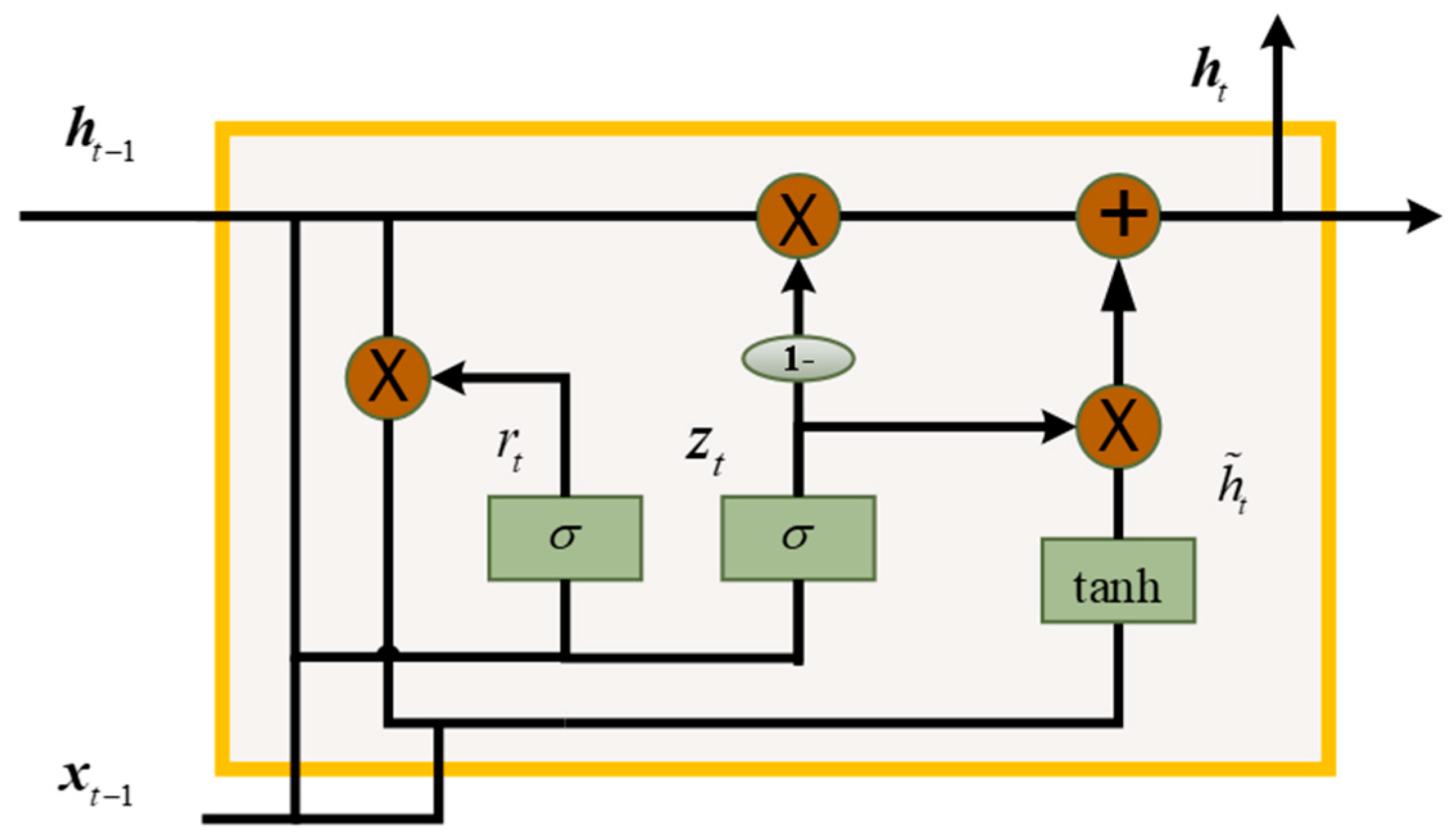
2.2. Gated Recurrent Unit (GRU)

The gated recurrent unit is another popular variant of the common RNN, and was first proposed by Cho in 2004 [32]. In a GRU, the information flow is also controlled and monitored based on a ‘gate’ structure, however, a GRU has no separate state cells. A GRU basic structure is shown in Figure 2. In the figure, ${\mathit{h}}_{t-1}$ is the hidden state at time $t-1$, and ${\mathit{h}}_t$ is the hidden state at time epoch $t$. The relationship between ${\mathit{h}}_{t-1}$ and ${\mathit{h}}_t$ is as Equation (6):

$${\mathit{h}}_t=\left(1-{\mathit{𝑧}}_t\right)\ast {\mathit{h}}_{t-1}+{\mathit{z}}_t\ast {\tilde{\mathit{h}}}_t$$

(6)

where ${\tilde{\mathit{h}}}_t$ is the candidate activation or hidden state, and the updating gate ${\mathit{𝑧}}_t$ decides how much the unit updates its hidden state, which is as Equation (7):

$${\mathit{𝑧}}_t=\sigma \left({\mathit{W}}_z\cdot \left[{\mathit{h}}_{t-1},{\mathit{x}}_t\right]\right)$$

(7)

where $\sigma (\cdot )$ is a sigmoid function, and determining the degree of the new hidden state will be added to the hidden state at time epoch $t$. In above, ${\mathit{W}}_z$ is the parameters which will be determined after training.

In addition, the new or candidate hidden state ${\tilde{\mathit{h}}}_t$ calculation is as Equation (8):

$${\tilde{\mathit{h}}}_t=tanh\left(\mathit{W}\cdot \left[{\mathit{r}}_t\ast {\mathit{h}}_{t-1},{\mathit{x}}_t\right]\right)$$

(8)

where ${\mathit{r}}_t$ is a set of reset gates, and when ${\mathit{r}}_t$ is close to 0, the unit acts as forgetting the previously computed state. ${\mathit{r}}_t$ is calculated as:

$${\mathit{r}}_t=\sigma \left({\mathit{W}}_r\cdot \left[{\mathit{h}}_{t-1},{\mathit{x}}_t\right]\right)$$

(9)

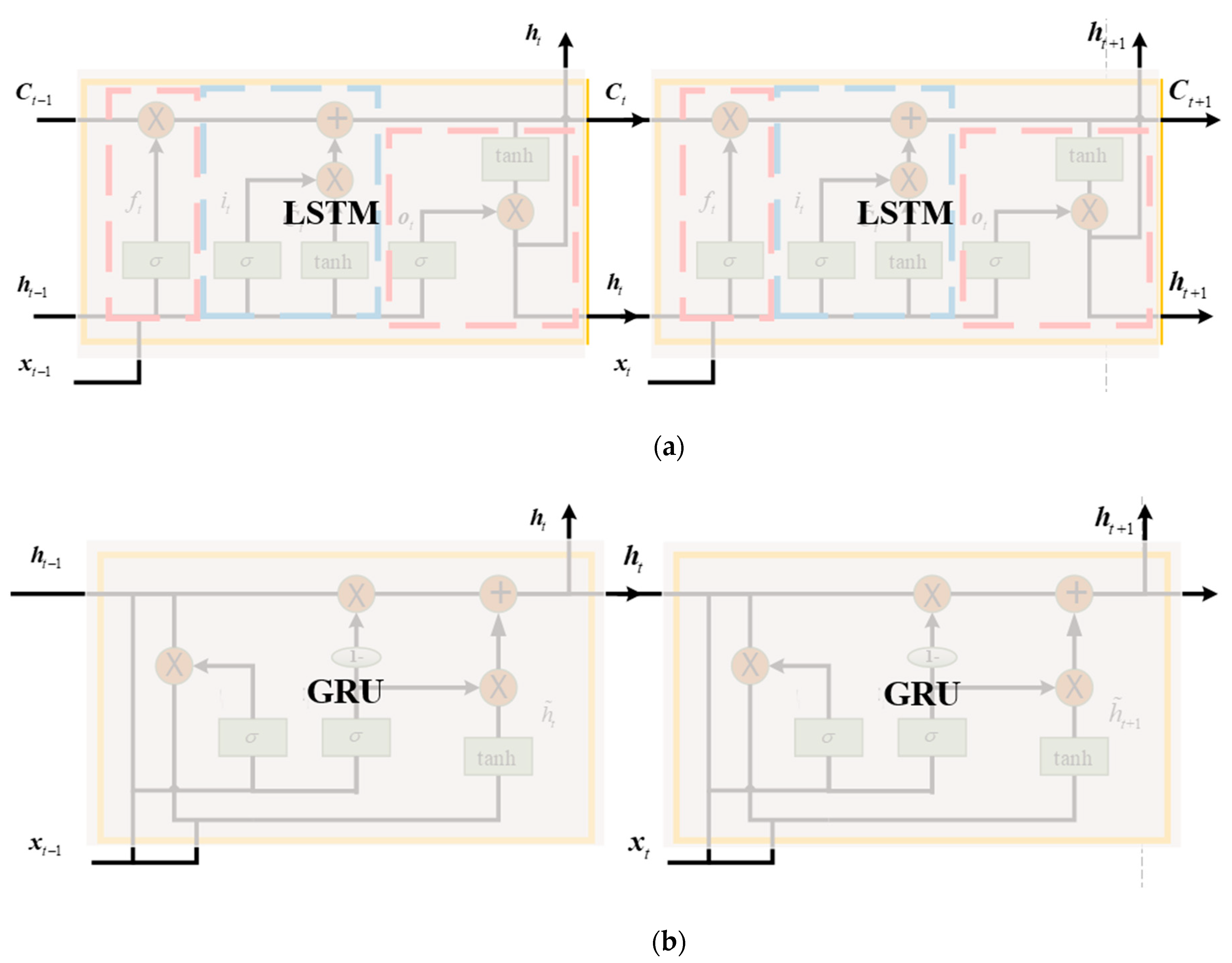
2.3. Mixed LSTM and GRU

As presented in Figure 1 and Figure 2, the LSTM and GRU are just a single unit. A deep LSTM-RNN or deep GRU-RNN is set up as Figure 3, the LSTM and GRU units are assembled and connected in the time domain, and the parameters propagation is also illustrated in detail. The output is determined by a LSTM or GRU sequence, thus, long term memory could also affect the current epoch output. Furtherly, Figure 4 presents the mixed LSTM and GRU deep RNN structures, Figure 4a shows the LSTM–GRU. In this structure, the cell state and hidden state are converted to the LSTM unit at the next epoch. The hidden state is also converted to the parallel GRU unit, and the hidden state propagates among the GRU units. In the GRU–LSTM structure (Figure 4b), the hidden state of GRU is converted to the next GRU unit and the parallel LSTM unit. Since the GRU has no cell state, in the mixed LSTM–GRU structure the cell state only propagates among the LSTM units.

3. Results

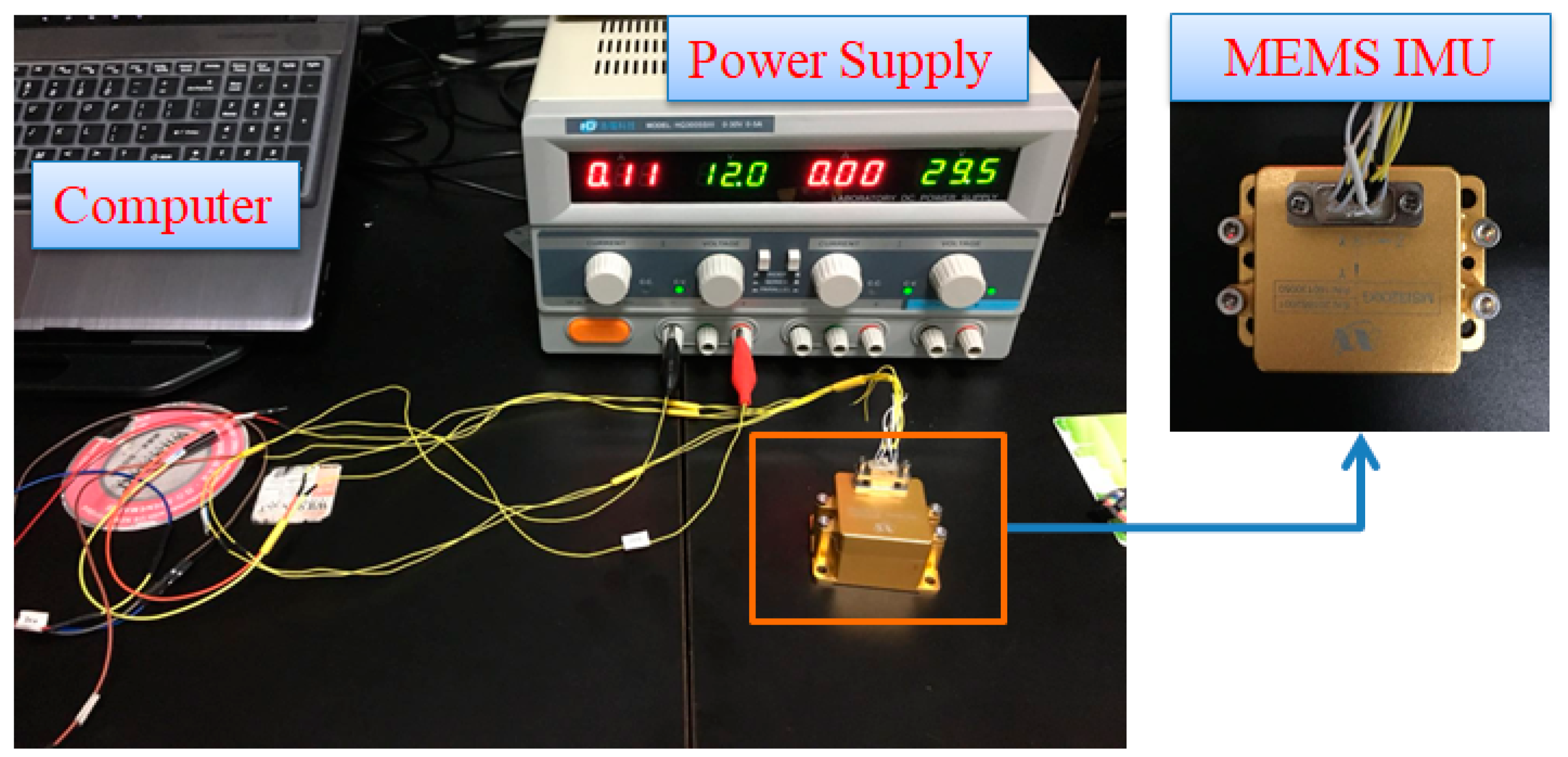
This section introduces the experimental setup and the results. Figure 5 presents the data collecting procedure; a MEMS IMU (MT Microsystem Company, Hubei, China) is employed, and the details are listed in

Table 1. Specifications of MSI3200 IMU.

MEMS IMU	Gyroscope	range	$\pm$300 °/s
		Bias stability (1 $\sigma$)	$\le$10 °/h
		Bias stability (Allan)	$\le$2 °/h
		Angle random walk	$\le$10 °/$\sqrt{h}$
	Accelerometer	range	$\pm$15 g
		Bias stability (1 $\sigma$)	0.5 mg
		Bias stability (Allan)	0.5 mg
	Power consumption	1.5 W
	Weight	250 g
	Size	$70\mathrm{mm}\times 54\mathrm{mm}\times 39\mathrm{mm}$
	Sampling rate	400 Hz

[33]. The MEMS IMU is same model that is employed in our previous paper, but they are not from the same batch [8]. Thus, they have similar parameters, but are actually different after precise calibration. This difference is caused by the MEMS manufacturing technology.

Figure 5 presents the data collecting equipment. The power supply delivers 12 V and 0.11 A while the MEMS IMU is connected. A computer is also connected to the MEMS IMU through a USB 2.0 cable. Control software is run by the computer to monitor the data collecting procedure, obtain, and store the data. The sampling frequency is set at 200 Hz, and the collecting time length is approximately 600 s.

The remainder of this section is divided into three sections: Section 3.1 illustrates the formulae of the gyroscope output data errors, the structure of the input, and output data for training and testing. Section 3.2 details the investigation of the training data length on the proposed mixed LSTM and GRU method, since the GRU had better performance with less training data length compared to the LSTM. The aim of the Section 3.2 was to explore the performance of the mixed LSTM and GRU RNN, as compared with multi-layer LSTM and multi-layer GRU. In Section 3.3, the performance of the new method was compared with the two-layer LSTM and two-layer GRU to provide a detailed description of the proposed method. Attitude errors are also presented for further comparison of these methods.

3.1. Input Data and Training

As illustrated in Figure 5, the gyroscope dataset was collected. The bias was calculated using the mean values of the collected data. After subtracting the bias, the processed dataset was labeled as $\mathit{X}=\left[x_1,x_2,x_3,\dots ,x_N\right]$. The subscript $N$ was termed as the number of input gyroscope samples. In the experiments, the dataset was divided into two parts: training part (${\mathit{X}}_{training}$) and testing part (${\mathit{X}}_{testing}$). The training dataset was employed to train the model, and the testing dataset was utilized to evaluate the performance of the trained model. The input vector of the RNNs could be described as:

$$\mathit{i}\mathit{n}\mathit{p}\mathit{u}{\mathit{t}}_i=\left[x_i,x_{i+1},\dots ,x_{i+step}\right],i\in \left[1,N_{training}-step\right]$$

(10)

where $\mathit{i}\mathit{n}\mathit{p}\mathit{u}{\mathit{t}}_i$ is the input vector of the RNNs and the variable $step$ is the length of the $\mathit{i}\mathit{n}\mathit{p}\mathit{u}{\mathit{t}}_i$ vector. The output vector $\mathit{o}\mathit{u}\mathit{t}\mathit{p}\mathit{u}{\mathit{t}}_i$ is described by:

$$\mathit{o}\mathit{u}\mathit{t}\mathit{p}\mathit{u}{\mathit{t}}_i=\left[x_{i+step+1}\right],i\in \left[1,N_{training}-step\right]$$

(11)

Equations (10) and (11) give the dataset for the training procedure, and the dataset in the testing step was similar to that of training procedure.

RNNs were trained using the errors back propagation method (BP). Since the RNNs were designed to process time series datasets, the BP method is termed BPTT (back-propagation through time) [36,37,38].

3.2. Comparison of LSTM–GRU and GRU–LSTM

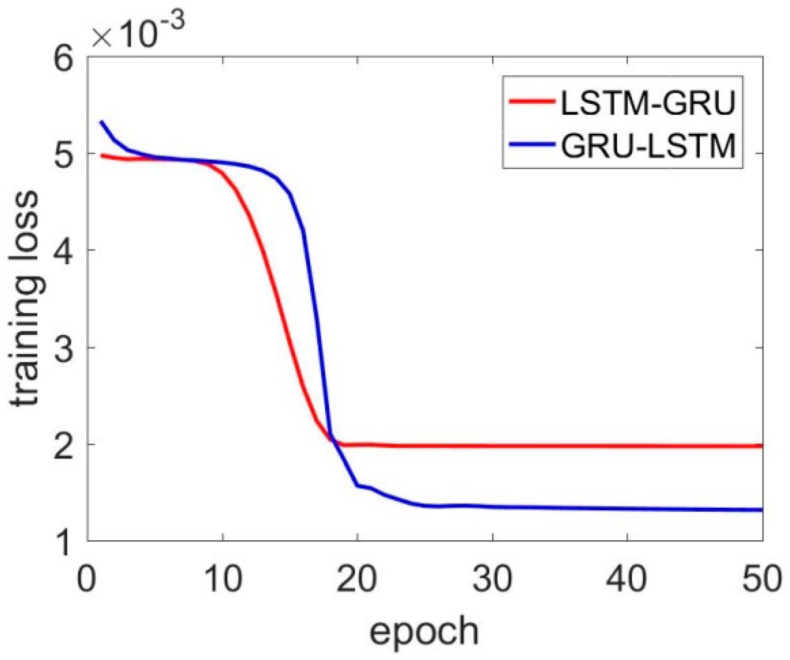
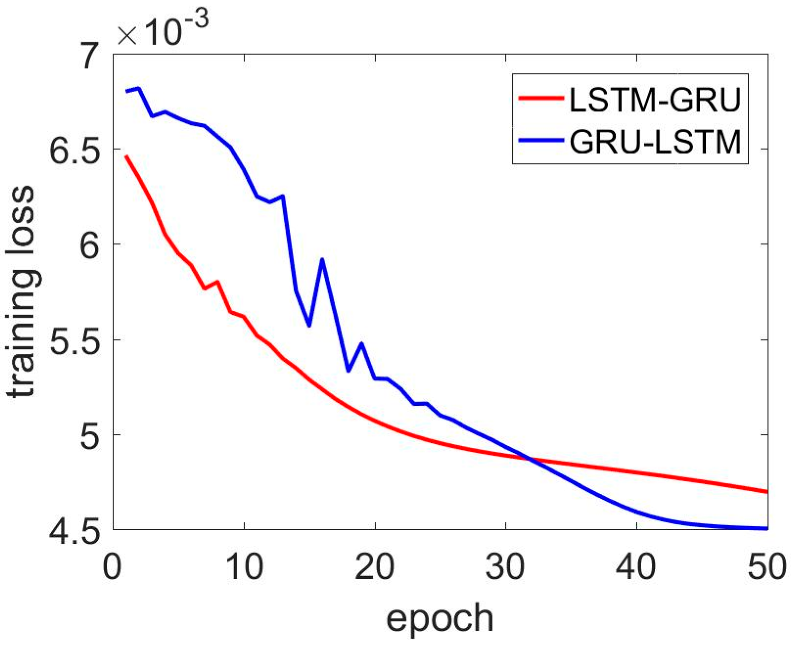
As aforementioned in Section 2.3, there were two different architectures in mixed LSTM and GRU. This section aimed to compare these two architectures in aspects of training loss and prediction accuracy. The date lengths of the training dataset and testing dataset were 1000 and 100,000, respectively. The learning rate was 0.01 for both, the hidden unit was 1, and the training epoch was 50. Figure 6, Figure 7 and Figure 8 present the training loss comparison of the LSTM–GRU and GRU–LSTM in the three-axis MEMS gyroscope de-noising. In addition, training loss means the errors between the predicted values and the real signal values were not included in the training dataset.

In these figures (Figure 6, Figure 7 and Figure 8), the red line represents the LSTM–GRU training loss, and the blue line represents the GRU–LSTM results. Figure 6 shows the x axis MEMS gyroscope results; the GRU–LSTM and LSTM–GRU both converged within 50 training epochs, but the GRU–LSTM delivered a lower convergence speed with smaller training loss. In Figure 7, the GRU–LSTM and LSTM–GRU seemed not to converge, while the LSTM–GRU had a better performance in reducing training loss. For the z axis MEMS gyroscope, LSTM–GRU converged fast to a stable value, while the GRU–LSTM did not converge within the set training epoch. We thought the difference was caused by the different architectures between LSTM–GRU and GRU–LSTM. LSTM-RNN had more parameters, which needed to be determined during the training procedure, When the LSTM was placed on the second layer, it was not sufficient for LSTM unit training. Overall, the LSTM–GRU was more feasible for this application, compared with the GRU–LSTM. Specifically, the prediction results are not presented, since the GRU–LSTM was not well trained with the settings.

3.3. Comparison of LSTM–GRU, Two-Layer LSTM, and Two-Layer GRU

This sub-section presents the comparison results from the two-layer LSTM, two-layer GRU, and the mixed LSTM–GRU.

Table 2. Standard deviation of gyroscope outputs (two-layer LSTM-RNN).

	X (degree/s)	Y (degree/s)	Z (degree/s)
Training loss	0.00132	0.00534	0.00139
LSTM-RNN	0.060	0.037	0.025
Original signals	0.069	0.083	0.047

,

Table 3. Standard deviation of gyroscope outputs (two-layer GRU-RNN).

	X (degree/s)	Y (degree/s)	Z (degree/s)
Training loss	0.00136	0.0055	0.00142
LSTM-RNN	0.059	0.034	0.026
Original signals	0.069	0.083	0.047

and

Table 4. Standard deviation of gyroscope outputs (mixed LSTM–GRU RNN).

	X (degree/s)	Y (degree/s)	Z (degree/s)
Training loss	0.00127	0.00469	0.00134
LSTM-RNN	0.060	0.035	0.0246
Original signals	0.069	0.083	0.047

show the training loss, standard deviation of the prediction results, and standard deviation of the raw MEMS gyroscope signals. In particular, the structure of the LSTM–GRU is shown in Figure 4. For the x axis gyroscope, the LSTM–GRU delivered the smallest training loss, however, the standard deviations of the de-noised signals were minor. In aspects of the y axis results, the training loss decreased by 12.2% and 14.7%, compared with that of the two-layer LSTM and two-layer GRU. However, the standard deviation of the de-noised signals did not show a significant improvement. For the z axis gyroscope results, the differences in the training loss between the two-layer LSTM, two-layer GRU, and LSTM–GRU were trivial.

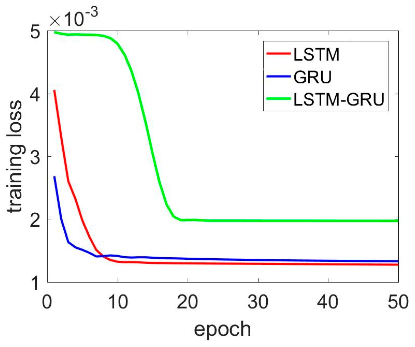
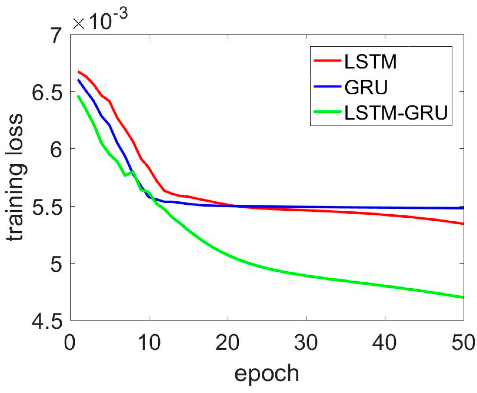
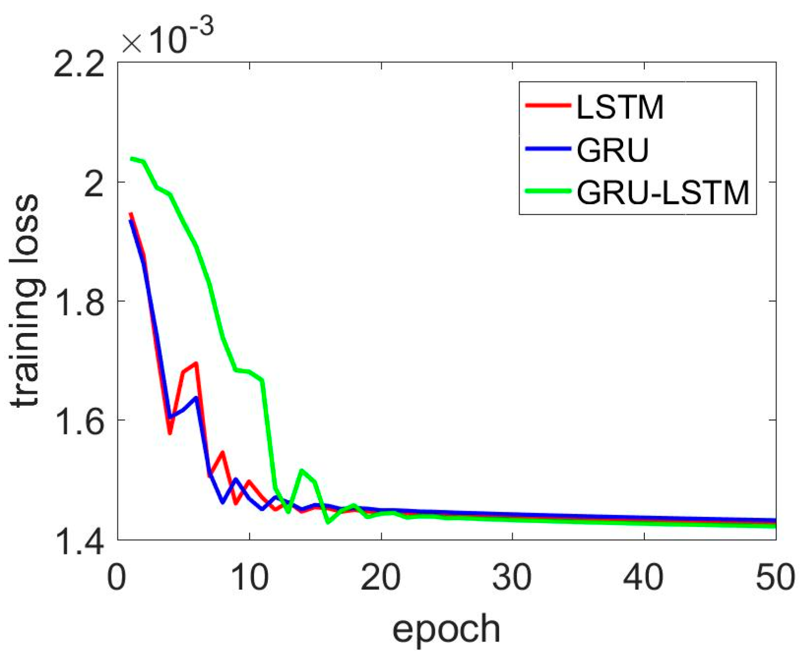
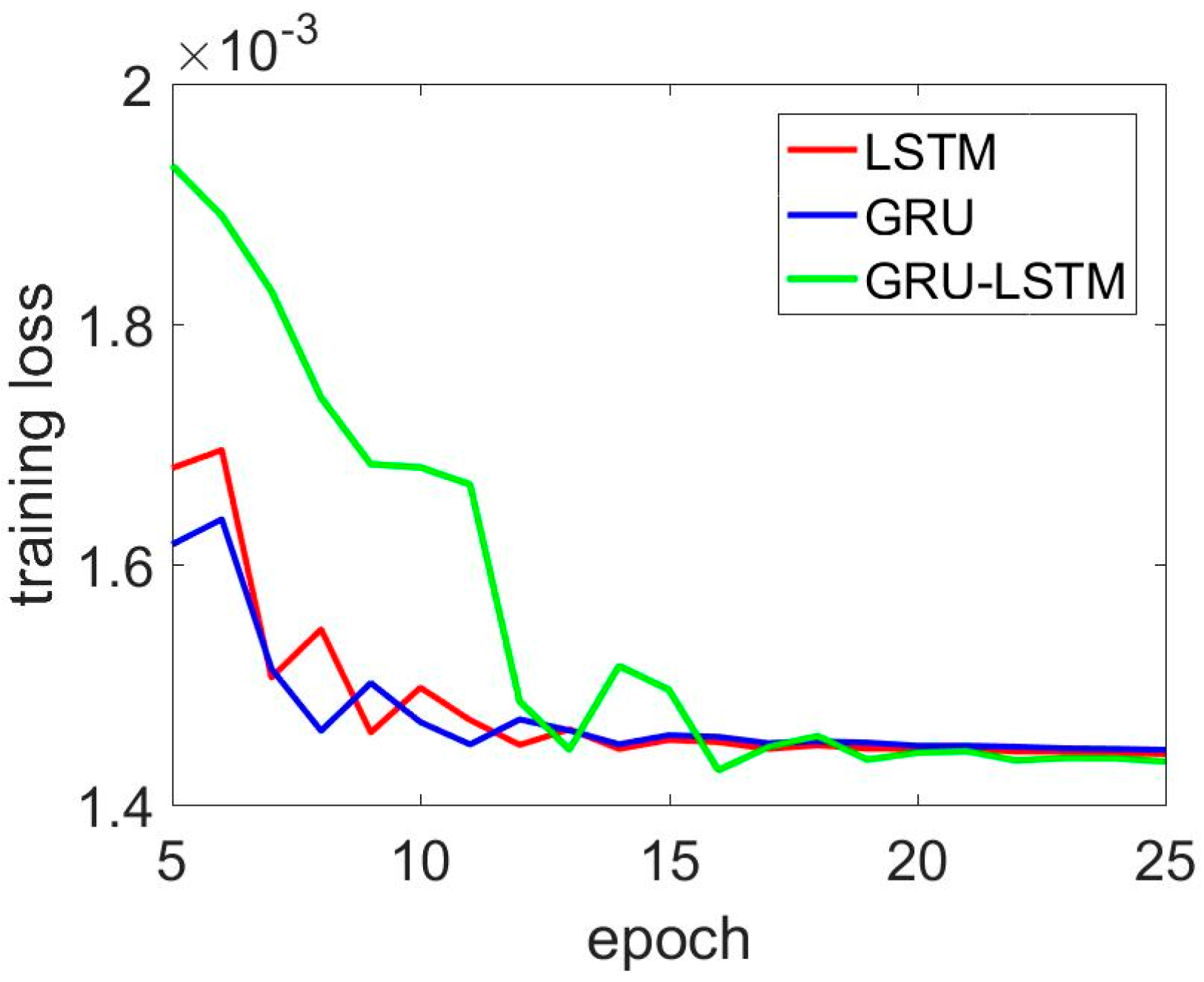
In addition, Figure 9, Figure 10, Figure 11 and Figure 12 present the detailed training losses during the training procedure. In these figures, the red line represents the training loss of the LSTM, the blue line shows the GRU results, and the last green line shows the LSTM–GRU training loss. Specifically, in Figure 9, the two-layer GRU and two-layer LSTM had better performance than the LSTM–GRU. For the LSTM–GRU, the training loss remained almost unchanging, and it converged quickly from the 10th to the 20th training epoch. In Figure 10, the LSTM–GRU outperformed the LSTM and GRU. Figure 11 and Figure 12 show the z axis gyroscope de-noised results. Figure 12 shows a magnified picture of the results from the 5th to the 20th epoch.

Basically, LSTM–GRU showed a slower convergence speed, especially the training epochs from 1 to 10. The phenomenon is obvious in Figure 9 and Figure 11. However, in Figure 10, the training loss of the LSTM–GRU was always below the two-layer LSTM and two-layer GRU. Moreover, the LSTM–GRU delivered smaller training loss than the two-layer LSTM and two layer GRU for the de-noised y axis and z axis gyroscope signals.

Furthermore,

Table 5. Attitude errors comparison.

	X (degree)	Y (degree)	Z (degree)
two-layer LSTM	0.136	0.240	0.184
two-layer GRU	0.167	0.215	0.205
LSTM–GRU	0.104	0.145	0.164
Original signals	0.382	0.473	0.394

presents the attitude errors comparison of the three recurrent neural networks (60 s). In Table 5, the three axes referred to pitch, roll, and yaw angles respectively. From the results, three major conclusions were obtained:

(1)

There was an obvious improvement in the attitude errors for all the three deep neural networks. The two-layer LSTM performed 64.4%, 49.3%, and 53.3% improvements in attitude errors, the two-layer GRU performed 56.3%, 54.5%, and 47.9% decreases in attitude errors, and the attitude errors of LSTM–GRU decreased by 72.2%, 69.3%, and 58.4%.

(2)

Specifically, for the x axis gyroscope data, LSTM–GRU had a large training loss, but the LSTM–GRU still showed 7.8% and 15.9% improvements compared with the two-layer LSTM and two-layer GRU. The minor difference of the standard deviation of the de-noised signals may account for this.

4. Discussion

In this paper, the influence of data length on the training performance was not presented and analyzed, as we were limited by the computer computation capacity. Longer training datasets might improve the performance of the deep recurrent neural network.

In the experiment, only static data were employed to evaluate the proposed method; a trajectory from field testing might be more feasible for sufficient testing.

As we were limited by computer capacity, only two-layer LSTM or GRU were employed and implemented in this paper. It may be meaningful to explore the LSTM or GRU with more layers.

5. Conclusions

In this paper, a proposed artificial intelligence method was employed and evaluated in MEMS three-axis gyroscope signal de-noising. Through the experiments, the following conclusions were obtained:

(1)

Two-layer LSTM, two-layer GRU, LSTM–GRU, and GRU–LSTM were effective for this application. The two-layer LSTM performed a 64.4%, 49.3%, and 53.3% improvement in attitude errors, the two-layer GRU performed a 56.3%, 49.3%, and 47.9% decrease in attitude errors, and the attitude errors of LSTM–GRU decreased by 72.2%, 69.3%, and 58.4%;

(2)

With a limited training dataset, LSTM–GRU outperformed GRU–LSTM; LSTM–GRU had a large training loss, but the LSTM–GRU still showed an improvement compared with the two-layer LSTM and two-layer GRU.

Future works might include: It might be meaningful to explore the LSTM and GRU with more layers, which might give better performance; a dynamic trajectory could be employed to evaluate the performance of the artificial intelligence in this application; as this paper deals only with MRMS gyroscope de-noising, artificial intelligence could be integrated with the GNSS/INS method to improve the accuracy during GNSS signal outages.

References

- Dow, J.M.; Ruth, E.N.; Chris, R. The international GNSS service in a changing landscape of global navigation satellite systems. J. Geod. 2009, 83, 191–198. [Google Scholar] [CrossRef]
- Montenbruck, O.; Steigenberger, P.; Khachikyan, R.; Weber, G.; Langley, R.B.; Mervart, L.; Hugentobler, U. IGS-MGEX: Preparing the ground for multi-constellation GNSS science. Inside GNSS 2014, 9, 42–49. [Google Scholar]
- Hewitson, S.; Wang, J. GNSS receiver autonomous integrity monitoring (RAIM) performance analysis. GPS Solut. 2006, 10, 155–170. [Google Scholar] [CrossRef]
- Lashley, M.; Bevly, D.M.; Hung, J.Y. Performance analysis of vector tracking algorithms for weak GPS signals in high dynamics. IEEE J. Sel. Top. Sign. Process. 2009, 3, 661–673. [Google Scholar] [CrossRef]
- Jiang, C.; Chen, S.; Chen, Y.; Bo, Y.; Wang, C.; Tao, W. Performance analysis of GNSS Vector tracking loop based GNSS/CSAC integrated navigation system. J. Aeronaut. Astronaut. Aviat. 2017, 49, 289–297. [Google Scholar]
- Chen, R.; Chen, Y.; Pei, L.; Chen, W.; Liu, J.; Kuusniemi, H.; Takala, J. A DSP-based multi-sensor multi-network positioning platform. In Proceedings of the 22nd International Technical Meeting of The Satellite Division of the Institute of Navigation, Savannah, GA, USA, 22–25 September 2009; pp. 615–621. [Google Scholar]
- Chen, Y.; Tang, J.; Jiang, C.; Zhu, L.; Lehtomäki, M.; Kaartinen, H.; Zhou, H. The accuracy comparison of three simultaneous localization and mapping (SLAM)-based indoor mapping technologies. Sensors 2018, 18, 3228. [Google Scholar] [CrossRef] [PubMed]
- Jiang, C.; Chen, S.; Chen, Y.; Zhang, B.; Feng, Z.; Zhou, H.; Bo, Y. A MEMS IMU de-noising method using long short term memory recurrent neural networks (LSTM-RNN). Sensors 2018, 18, 3470. [Google Scholar] [CrossRef]
- Chiang, K.W.; Huang, Y.W. An intelligent navigator for seamless INS/GPS integrated land vehicle navigation applications. Appl. Soft Comput. 2008, 8, 722–733. [Google Scholar] [CrossRef]
- Chiang, K.W.; Duong, T.T.; Liao, J.K. The performance analysis of a real-time integrated INS/GPS vehicle navigation system with abnormal GPS measurement elimination. Sensors 2013, 13, 10599–10622. [Google Scholar] [CrossRef]
- Syed, Z.F.; Aggarwal, P.; Goodall, C.; Niu, X.; El-Sheimy, N. A new multi-position calibration method for MEMS inertial navigation systems. Meas. Sci. Technol. 2007, 18, 1897. [Google Scholar] [CrossRef]
- Cho, S.Y.; Park, C.G. MEMS based pedestrian navigation system. J. Navig. 2006, 59, 135–153. [Google Scholar] [CrossRef]
- Brown, A.K. GPS/INS uses low-cost MEMS IMU. IEEE Aerosp. Electron. Syst. Mag. 2005, 20, 3–10. [Google Scholar] [CrossRef]
- Jiang, C.H.; Chen, S.; Chen, Y.Y.; Bo, Y.M. Research on chip scale atomic clock driven GNSS/SINS deeply coupled navigation system for augmented performance. IET Radar. Sonar Navig. 2018. [Google Scholar] [CrossRef]
- Ning, Y.; Wang, J.; Han, H.; Tan, X.; Liu, T. an optimal radial basis function neural network enhanced adaptive robust Kalman filter for GNSS/INS integrated systems in complex urban areas. Sensors 2018, 18, 3091. [Google Scholar] [CrossRef] [PubMed]
- Niu, X.; Nassar, S.; El-Sheimy, N. An accurate land-vehicle MEMS IMU/GPS navigation system using 3D auxiliary velocity updates. Navigation 2007, 54, 177–188. [Google Scholar] [CrossRef]
- Li, W.; Wang, J. Effective adaptive Kalman filter for MEMS-IMU/magnetometers integrated attitude and heading reference systems. J. Navig. 2013, 66, 99–113. [Google Scholar] [CrossRef]
- Bhatt, D.; Aggarwal, P.; Devabhaktuni, V.; Bhattacharya, P. A novel hybrid fusion algorithm to bridge the period of GPS outages using low-cost INS. Expert Syst. Appl. 2014, 41, 2166–2173. [Google Scholar] [CrossRef]
- El-Sheimy, N.; Hou, H.Y.; Niu, X.J. Analysis and modeling of inertial sensors using Allan variance. IEEE Trans. Instrum. Meas. 2008, 57, 140–149. [Google Scholar] [CrossRef]
- Allan, D.W. Historicity, strengths, and weaknesses of Allan variances and their general applications. Gyroscopy Navig. 2016, 7, 1–17. [Google Scholar] [CrossRef]
- Radi, A.; Nassar, S.; El-Sheimy, N. Stochastic error modeling of smartphone inertial sensors for navigation in varying dynamic conditions. Gyroscopy Navig. 2018, 9, 76–95. [Google Scholar] [CrossRef]
- Aggarwal, P.; Syed, Z.; Niu, X.X.; EI-Sheimy, N. A standard testing and calibration procedure for low cost MEMS inertial sensors and units. J. Navig. 2008, 61, 323–336. [Google Scholar] [CrossRef]
- Wang, D.; Dong, Y.; Li, Q.; Li, Z.; Wu, J. Using Allan variance to improve stochastic modeling for accurate GNSS/INS integrated navigation. GPS Solut. 2018, 22, 53. [Google Scholar] [CrossRef]
- Zhang, Q.; Wang, X.; Wang, S.; Pei, C. Application of improved fast dynamic Allan variance for the characterization of MEMS gyroscope on UAV. J. Sens. 2018. [Google Scholar] [CrossRef]
- Wang, L.; Zhang, C.; Gao, S.; Wang, T.; Lin, T.; Li, X. Application of fast dynamic Allan variance for the characterization of FOGs-Based measurement while drilling. Sensors 2016, 16, 2078. [Google Scholar] [CrossRef] [PubMed]
- Su, W.P.; Hao, Y.S.; Li, Q.C. Arma-akf model of mems gyro rotation data random drift compensation. Appl. Mech. Mater. 2013, 321–324, 549–552. [Google Scholar] [CrossRef]
- Huang, L. Auto regressive moving average (ARMA) modeling method for Gyro random noise using a robust Kalman filter. Sensors 2015, 15, 25277–25286. [Google Scholar] [CrossRef] [PubMed]
- Khashei, M.; Bijari, M. A novel hybridization of artificial neural networks and ARIMA models for time series forecasting. Appl. Soft Comput. 2011, 11, 2664–2675. [Google Scholar] [CrossRef]
- Waegli, A.; Skaloud, J.; Guerrier, S.; Parés, M.E.; Colomina, I. Noise reduction and estimation in multiple micro-electro-mechanical inertial systems. Meas. Sci. Technol. 2010, 21, 156–158. [Google Scholar] [CrossRef]
- Bhatt, D.; Priyanka, A.; Prabir, B.; Vijay, D. An enhanced mems error modeling approach based on nu-support vector regression. Sensors 2012, 12, 9448–9466. [Google Scholar] [CrossRef]
- Xing, H.F.; Hou, Bo.; Lin, Z.H.; Guo, M.F. Modeling and compensation of random drift of MEMS gyroscopes based on least squares support vector machine optimized by chaotic particle swarm optimization. Sensors 2017, 17, 2335. [Google Scholar] [CrossRef]
- Jiang, C.; Chen, S.; Chen, Y.; Bo, Y.; Han, L.; Guo, J.; Feng, Z.; Zhou, H. Performance Analysis of a Deep Simple Recurrent Unit Recurrent Neural Network (SRU-RNN) in MEMS Gyroscope De-Noising. Sensors 2018, 18, 4471. [Google Scholar] [CrossRef]
- Understanding LSTM Networks. Available online: https://colah.github.io/posts/20150–8-Understanding-LSTMs/ (accessed on 27 August 2015).
- Hosseinyalamdary, S. Deep Kalman filter: Simultaneous multi-sensor integration and modelling; A GNSS/IMU case study. Sensors 2018, 18, 1316. [Google Scholar] [CrossRef] [PubMed]
- Chung, J.; Gulcehre, C.; Cho, K.; Bengio, Y. Gated feedback recurrent neural networks. In Proceedings of the International Conference on Machine Learning, Lille, France, 6–11 July 2015; pp. 2067–2075. [Google Scholar]
- Gers, F.A.; Schraudolph, N.N.; Schmidhuber, J. Learning precise timing with LSTM recurrent networks. J. Mach. Learn. Res. 2002, 3, 115–143. [Google Scholar]
- Ordóñez, F.J.; Roggen, D. Deep convolutional and LSTM recurrent neural networks for multimodal wearable activity recognition. Sensors 2016, 16, 115. [Google Scholar] [CrossRef] [PubMed]
- MSI3200. Available online: http://www.mtmems.com/product_view.asp?id=28 (accessed on 5 August 2017).
Figure 1.
Basic structure of a long short term memory (LSTM) unit.
Figure 2.
Basis structure of a gate recurrent unit (GRU).
Figure 3.
Deep LSTM and GRU with single layers. (a) A single layer LSTM; (b) a single layer GRU.
Figure 4.
Structures of the mixed LSTM and GRU. (a) LSTM–GRU; (b) GRU–LSTM.
Figure 5.
MEMS Gyroscope data collecting procedure.
Figure 6.
LSTM–GRU and GRU–LSTM training loss for the x axis gyroscope.
Figure 7.
LSTM–GRU and GRU–LSTM training loss for the y axis gyroscope.
Figure 8.
LSTM–GRU and GRU–LSTM training loss for the z axis gyroscope.
Figure 9.
LSTM, GRU, and LSTM–GRU training loss comparison for x axis gyroscope.
Figure 10.
Figure 11.
LSTM, GRU, and LSTM–GRU training loss comparison for z axis gyroscope.
Figure 12.
Zooming out of Figure 11 from the 5th to 25th epoch.