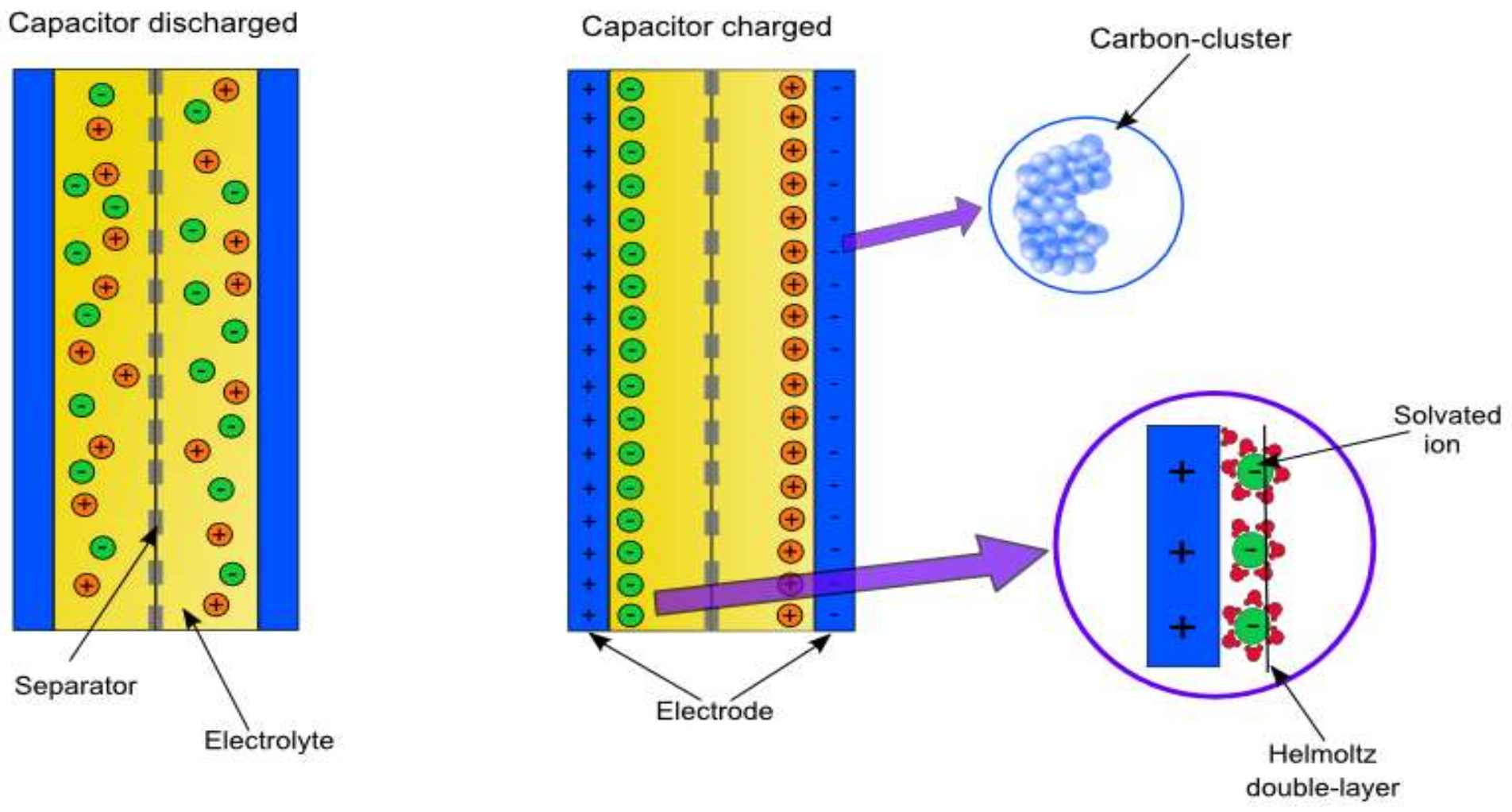
Article

Supercapacitor Electro-Mathematical and Machine Learning Modelling for Low Power Applications

by
Borja Pozo
1,*,
Jose Ignacio Garate
2,
Susana Ferreiro
1,
Izaskun Fernandez
1 and
Erlantz Fernandez de Gorostiza
1
1
Electronics and Communications Unit and Intelligent Information System Unit, IK4-Tekniker, Calle Iñaki Goenaga 5, 20600 Eibar, Spain
2
Department of Electronics Technology, University of the Basque Country (UPV/EHU), 48080 Bilbao, Spain
*
Author to whom correspondence should be addressed.
Electronics 2018, 7(4), 44; https://doi.org/10.3390/electronics7040044
Submission received: 9 February 2018 / Revised: 22 March 2018 / Accepted: 28 March 2018 / Published: 29 March 2018
(This article belongs to the Special Issue Energy Harvesting for Smart Sensing System and IoT)

Abstract

:
Low power electronic systems, whenever feasible, use supercapacitors to store energy instead of batteries due to their fast charging capability, low maintenance and low environmental footprint. To decide if supercapacitors are feasible requires characterising their behaviour and performance for the load profiles and conditions of the target. Traditional supercapacitor models are electromechanical, require complex equations and knowledge of the physics and chemical processes involved. Models based on equivalent circuits and mathematical equations are less complex and could provide enough accuracy. The present work uses the latter techniques to characterize supercapacitors. The data required to parametrize the mathematical model is obtained through tests that provide the capacitors charge and discharge profiles under different conditions. The parameters identified are life cycle, voltage, time, temperature, moisture, Equivalent Series Resistance (ESR) and leakage resistance. The accuracy of this electro-mathematical model is improved with a remodelling based on artificial neuronal networks. The experimental data and the results obtained with both models are compared to verify and weigh their accuracy. Results show that the models presented determine the behaviour of supercapacitors with similar accuracy and less complexity than electromechanical ones, thus, helping scaling low power systems for given conditions.

1. Introduction

Portable and autonomous electronic devices are becoming increasingly popular. One of their major drawbacks is their dependence on batteries [1,2]. Thus, battery life is a critical design factor, especially when wireless capabilities are required, because it involves a high percentage of total consumption by the WSN [3,4]. One technique to store the harvested energy and increase the amount of energy available is using supercapacitors or Electric Double Layer Capacitors (EDLC). They are attractive because they have higher power density than batteries, do not require special charging circuitry, and have a long operational lifetime. In order to minimize or optimize the power consumption, supercapacitors on energy harvesting systems must act as a primary storage device with a battery backup whenever it is necessary [5]. The benefits of using supercapacitors are many, like extended battery life, less electromagnetic interferences and better operation of analogic electronics. They are explained at length in the literature [6,7].
The first step to select a supercapacitor is based on the dimension the capacitance and form factor for the target application, which requires a complete characterization of the power consumption pattern of the target application. This information determines the size of the supercapacitor and whether if primary or secondary battery backup is needed. However, supercapacitors can not be analysed based only on their capacitance. Load current drain patterns, work cycle and temperature conditions change the characteristics of charge and discharge profiles [8]. The previous statement is especially true regarding low power applications because changes occur more often. Therefore, when the application must optimize the last drop of energy harvested, even in extreme conditions, a simple model of supercapacitors is not enough to estimate the real energy store capacity of the supercapacitor, i.e., the capacitance and its dynamic behaviour. The energy consumption pattern is a variable that depends on the application and the amount of available harvested energy, and it can be estimated statistically (windmills, solar panels indoors, etc.) [9]. This information and an accurate enough supercapacitor model will allow determining the required capacitance value for different conditions.
Electrochemical models can be found in [10,11]; these studies and models use complex equations and rely on electrochemical theory based on physical principles shown in Figure 1. Moreover, the parameters used in these equations are difficult to obtain because they require complex, expensive measurement equipment and long measurement times. Despite this complexity, up to date, these models usually provide the best accuracy.
The purpose of this paper is to define a complete model to analyse the charge and discharge behaviour of a supercapacitor with an accuracy equivalent to that of the electromechanical models. Two different techniques have been used to reach the aforementioned objective, one electro-mathematical equations based and another with machine learning algorithms. Besides, these models could provide information of the supercapacitors for low power systems without using complex electrochemical models.

2. Related Work at Different Techniques

Dimension of the power system requirements of a low power electronic system involves characterising the nonlinear behaviour of the supercapacitor [12]. Supercapacitor charging and discharging does not present the same behaviour as standard capacitors because the leakage currents are a function of the charge and discharge dynamics [13]. Unless characterization of capacitors is done best, theoretically, with electromechanical models, nonetheless, there are another two lines of research and modelling of supercapacitor, mathematical integro-differential equation-based and IA. There is also a third approach that uses an approximate equivalent electrical model.

2.1. Equivalent Electrical Model

Capacitor ideal and simplified models of Figure 2a,b do not suffice for supercapacitor characterization [14]. Thus, as with standard capacitors like tantalum or electrolytic [15], it could use an equivalent electrical model of distributed components, Figure 2c, based on the physic morphology of the supercapacitor [16,17].
The electrical model represented in Figure 2c uses a distributed capacitance architecture in which each capacitance branch has a capacitance equation that emulates a particular physical behaviour. The coefficients of these equations are obtained empirically. The dynamic characteristic of supercapacitor and its nonlinear leakage current behaviour limit the advantages of this model. There are studies that have tried to improve this model with more complex and elaborate RC nets [18].

2.2. Mathematical Model

The physical structure, chemistry reactions and current distribution inside the capacitor could be modelled through mathematical expressions. These models characterise the non-linear behaviour of the leakage current, which is a function of the discharge dynamic pattern and the internal chemistry of the device.
A full electrochemical model of self-discharge studies the reactions on the electrode surface, through which electrons cross its double layer, as per the rule of the leakage and mathematical model of [19]. The model combines quantum mechanical and electrochemical phenomena that occur in the self-discharge process. Once the model is defined, it employs a computational method to simulate the discharge profile and energy storage for blocking layers of different thickness. Another alternative to obtain a mathematical model is presented in [20]. This research uses a different approach; it applies Lie derivate and Kalman filter to analyse the ion mobility and, thus, develops a supercapacitor electrochemical model with an observer.
Mathematical models take several critical parameters and show how this concrete parameter affect the operation of the device. Models of these types are less complex to implement than models based on electrochemical equations. e.g., at [21] the state of charge estimation is realized considering charge redistribution in real-time systems as EHWSN. Implementation of such a model without complex electrochemical equations provides good accuracy because it requires low memory usage and has low computational cost.

2.3. Machine Learning Algorithms

Machine learning as defined in [22] is a subfield of artificial intelligence closely related to data mining. Its aim is to develop algorithms that allow the machines to learn from data, i.e., to create programs able to induce models that improve their performance with the incoming data flow over time. It mixes mathematical elements with statistics and computational sciences such as classification trees, induction rules, neural networks, Bayesian networks, regression algorithms, supported vector machines or clustering [23].
Artificial Neural Network (ANN) is a mathematical computational model, which processes the information like biological neural systems such as the brain. It consists of a group of interconnected artificial neurons, which solves problems working in unison and processing information by means of a connectionist approach to computation. An ANN is an adaptive system that changes its structure based on information that flows through the neural network over the learning or training phase. The aforementioned phase involves adjusting the existing synaptic connections between neurons, thus, updating the network architecture and the connection weights.
ANN is one of the most widespread learning algorithms used within machine learning to model complex nonlinear relationships between inputs and outputs and find patterns in data. Its increasing popularity is due to its seemingly low dependence on any domain-specific knowledge and the availability of efficient learning algorithms, computational power, ability to model any given function, convergence speed and statistics. For this reason, ANN has been successfully applied to a broad spectrum of data-intensive applications.
In literature, there are some examples that use machine learning models to characterize some parameters of capacitor and energy storage devices. Work in [23] develops an algorithm for automotive applications that has one-layer feed forward ANN. This ANN is trained using a back-propagation algorithm that takes into account temperature, chemistry and life cycle. The work presented in [24] implements a current impedance test using machine learning. This test set-up presents an equivalent circuit base on the theory of electrochemical impedance spectroscopy that defines a first-phase linear model. In a second step, a multi-layer of Artificial Neuronal Network (ANN) establishes relationships among non-linear parameters of the capacitances and resistances. The aforementioned ANN is trained with experimental data banks using a back-propagation algorithm. Combining ANN and the equivalent circuit, the author can create an online nonlinear dynamic model. The research of [25] models a hybrid energy storage system for a Toyota Rav4EV with a stochastic nonlinear predictive control. Power demand is modelled as a Markov chain that had been trained with real-world driving cycles and simulation results given with a model in the loop.

3. Experimental Tests

Both models are verified and debugged through the experimental test set-ups: Furthermore, the tests also provide the charge current profile for the mathematical model. Then, obtained results are used later for the training and verification processes of the machine learning algorithms.
As described and referenced in section I, the behaviour of a supercapacitor is quite sensitive to several parameters. The following steps were used to certify and guarantee that the measurements are valid.
  • Define the number of tests and their conditions and the measurement procedure.
  • Design and build an evaluation fixture for testing different supercapacitors simultaneously.
  • Implement the tests and obtain results.

3.1. Test Definition

The number and type of test conditions are applied to variables or parameters are shown in Table 1.
With this set of variables, 15 charge tests and 21 discharge tests have been implemented for each supercapacitor. Each test condition is reproduced in a climatic chamber. The test starts when the conditions are stabilized, and the power supply is turned on.
Once the power supply is turned on, the supercapacitor starts its charge. The charge process is isolated from the load to prevent energy losses. When the charge finishes, the power supply is disconnected from the supercapacitor. At this point, if there is no load, the self-discharge through the supercapacitor internal resistance starts. Different discharge profiles are obtained connecting an electronic load to the capacitor. The load discharge profile chosen ranges from a single constant discharge step up to five different constant discharge steps. This number is considered necessary to verify the mathematical and machine learning model, which may be of n stages.

3.2. Evaluation-Board

Figure 3b shows the evaluation board which is made of four test fixtures. The schematic of each text fixture is the same. The test circuit of Figure 3a has two switches and uses the following three states:
  • Charging: first switch on and second off.
  • Self-discharge process: with the capacitor in charge state, the first switch is turned off.
  • Load dependent discharge process: with the capacitor in charge state, the first switch is turned off and the second on.
This switched architecture emulates an energy-harvesting environment and prevents instantaneous charge of the supercapacitor. The circuit has a current limiter resistor of 100 Ω at the input that limits the maximum charging current to 50 mA. The load is modelled with a variable resistance, and the voltage is regulated with a low dropout voltage regulator of 2 V minimum input operation voltage (TPS79730-EP).
Unless the evaluation board has four capacitors, the measurement data obtained with two capacitors is enough to build, verify and validate the mathematical and machine learning model, the remain two are used to further verify the test. Therefore, the data present in this work comes from the models PM-5R0H105-R of 1 F and PHV-5R4H505-R of 5 F.

3.3. Test Results

The measurements of the charge current, charge and discharge voltage are obtained with a data logger switch unit, model 34970A and data acquisition periods of 1 s. The test set-ups results are summarised in Figure 4 and Figure 5. Traces of Figure 4 show the charge and discharge profiles of the two aforementioned supercapacitors under test for a fix charging time of 600 s and voltage of 5 Volts, at four operation temperatures of 10, 25, 40 and 60 °C. The results show that the temperature impact on the supercapacitor charge and discharge profiles increases as its capacitance value decreases. Electron movement is slower as the temperature decreases, which reduces the discharge rate. As the temperature builds up, the movement of internal electrons are faster, thus the number of the electrochemical reactions is higher, and therefore, the discharge rate increases.
Another test results are completed with the traces of Figure 5 that provide the charge and discharge profiles of the two supercapacitors tested when the temperature conditions, the charging time, the load and the discharge pattern change. The profiles selected are quite different in order to validate the mathematical model for different ambient conditions and ranges. The results show that:
  • The supercapacitor discharge curves are a function of the load and the discharge time.
  • Changes of the ambient conditions and load produce significant deviation of the discharge characteristic.
  • The accuracy of the machine learning model is a direct function of the amount data.

4. Electro-Mathematical Model

The mathematical model selected is based in integro-differential equations. The electro-mathematical model presented combines the equations of [26,27,28,29,30,31,32]. As has been aforementioned in section II, the existing electro-mathematical models [26,27,28,29,30,31,32] implement only one or two parameters, which produces a limited model. The present work increases the number of parameters (capacitance life cycle, voltage, time, temperature, moisture, ESR, and leakage resistance) to characterize the supercapacitor behaviour and integrates them in a single model. Combining different parameters at the same time may produce unexpected or unwanted effects with an unknown root cause, therefore, the parameters are inserted and analysed one at a time to isolate and determine the origin of these issues whenever they occur.

4.1. Equations

Electro-mathematical model employs two equations [26], one for charge (Equation (1)) and one for discharge (Equation (2)). These equations create an exponential increase/decrease curve for each case, which are principles of the operation mode.
V c h a r g e = I c h a r g e × R e s r + I c h a r g e × R l e a k × ( 1 e ( t R l e a k × C c o m p l e t ) )
V d i s c h a r g e = V c h a r g e I d i s c h a r g e × R e s r ( V d i s c h a r g e 1 + I d i s c h a r g e × R l e a k ) × ( 1 e ( t R l e a k × C c o m p l e t ) )
where Vcharge/Vdischarge is the charge/discharge value of the supercapacitor in Volts, Icharge/Idischarge is the profile of charge/discharge current in Amperes, Resr is the equivalent series resistance in ohms, Rleak is the internal high resistance (leakage resistance) in ohms, Ccomplet de capacitance of the supercapacitor in Farads and T the time in seconds. Ccomplet, Resr and Rleak values are a function of the ambient conditions, lifetime, applied voltage, moisture, etc.

4.1.1. Capacity Ccomplet

Supercapacitor full capacity is obtained multiplying the percent of change that life cycle introduces in theoretical nominal capacitance,
C c o m p l e t = C 0   ( F ) × C c y c l e l i f e ( % )
Capacitor lifetime decreases with increasing temperature, applied voltage, humidity, current and backup time requirements [27,28]. Therefore, operation at high temperature reduces the life of a device. According to the “10-degrees-rule”, lifetime of supercapacitor will be double for each 10 °C reduction in operating temperature. This rule employs the Arrhenius equation, a formula for the temperature dependence of reaction rates. Likewise, lifetime diminishes as operation time increases. In a supercapacitor, the internal capacity decreases by the root of cycles [29]. Moreover, this type of device has a single voltage range, therefore, if this level is exceeded, life cycle decreases, and eventually the device may break. Finally, the last parameter included in the present work life cycle equation is moisture. Unless this environmental condition has less affection than the other parameters, it is included in the equation to improve the accuracy of the algorithm for a real low power application. Thus, the capacitor lifetime is:
C c y c l e l i f e ( % ) = 100 α ( T T r e f 10 ) × N × ( V V c V ) × H
where, α is acceleration factor, (usually α equal 2 for this type of applications), T is the actual operation temperature in Kelvin degrees, Tref is the reference operation temperature (usually 298 K), N is the number of cycles used, V is the voltage range, Vc is the applied voltage, both in Volts, and H is the percent of ambient moisture.

4.1.2. Equivalent Series Resistance

Equivalent Series Resistance (ESR) of supercapacitor is a function of temperature and device size [30]. The ESR increases as the temperature decreases. Consequently, when supercapacitor is operating at low temperature, its discharge efficiency diminishes. The ESR equation employed is:
R e s r = b 1 × R e s r 0 × ( 1 + γ × ( T T r e f ) ) + b 2 × R e s r 0 × e ( ( K t 2 ) × ( T T r e f ) )
where T0 = 293 K, γ = 0.007 (K−1) the temperature coefficient of the aggregated aluminium and carbon constituents and kT = 0.045 (K−1) the aggregate ionic activation energy constituent. The electronic (b1) and ionic (b2) weight factors are function of the supercapacitor cell size. Smaller cells have higher imbalance in the electronic to ionic ratio, in this case b1 is a larger fraction of b1 + b2 = 1 [31]. Resr0, is the theoretical series resistance and must be measured if the manufacturer does not provide the value.

4.1.3. Leakage Resistance

A supercapacitor usually has a high internal resistance, which implies a low leakage current, i.e., the current needed to keep the capacitor charged is low. When the capacitor is disconnected from the source, it begins to lose charge through the internal or leakage resistance. Manufacturers do not usually provide internal resistance information. Moreover, it is a parameter that is hard to measure. This work uses equation 6 [32], to obtain the instantaneous theoretical or approximate leakage resistance value, Rleak.
R l e a k = τ l e a k C c o m p l e t + k × u ( t ) = τ l e a k C c o m p l e t + ( 2 ( I Δ t t C c o m p l e t Δ U t ) Δ U t 2 ) × U 0 e ( t τ l e a k )
where τleak is the time constant of leakage current, k is the linear voltage-dependent capacitance and u(t) is voltage across the capacitor over time and is an exponential function where U0 is the initial voltage. The slope k is defined by the evolution of voltage ΔUt with time and the stored charge on the supercapacitor.

4.2. Model Architecture

The aforementioned Equations (1) and (2) require post processing, Figure 6, to obtain their coefficients and define the capacitor equivalent curves. In order to simulate the desired operation conditions, the variables and the charge current profile, i.e., a data file, must be introduced manually in the equations.
The first step defines the capacitor charging process. Temperature, moisture, life cycle state, ESR theoretical resistance are introduced and the configuration charge voltage and time are inserted on Equation (1) and the program provides the charge curve.
The second step defines the discharge profile. There are two alternatives to define the discharge profile. The self-discharge one only uses the internal losses of supercapacitors. It describes how long the self-discharge discharge process takes, (usually a large period of time), and which is the amount of energy lost under different ambient conditions; thus, it does not require additional configuration parameters. The second option employs different loads to create discharge profiles, (those found in EHWSN applications as reference of low power system), therefore, for each discharge profile test performed, load and time step must be defined.
The complete mathematical model was implemented in MATLAB®. It has a different algorithm for each case based on the aforementioned principles. All these algorithms have been integrated in a single program where the user can select the desired test set-up.

4.3. Results

This new electro-mathematical model is post-processed at different conditions of voltage, current, power and energy levels to analyse its performance and verify its accuracy. Figure 7 and Figure 8 summarizes the results of test set-ups devised through the charge and discharge profiles of the two reference supercapacitors under test. Figure 7 provides the effects for different load consumption discharge profiles on the behaviour of the same and different supercapacitor at the same temperature. Figure 8 presents how changing the temperature affects the supercapacitor’s storage capacity having the same load consumption discharge profile and shows which supercapacitor value goes into critical working level.

5. Machine Learning Model

Artificial Neural Networks (ANN) algorithms is one algorithm to improve the accuracy of mathematical models. The machine learning model defined in this work is used to predict the charge and discharge curves of supercapacitors for the low power application field based on the electro-mathematical model and test measurements described in the previous section.

5.1. Artificial Neural Network Setup

One of the most commonly used families of Artificial Neural Networks is the feed-forward network, where connections between the neurons do not form a directed cycle. In this type of network, the information moves only in one direction, forward, from the input nodes, through the hidden nodes (if any) to the output nodes. Cycles or loops in the aforementioned ANN network do not exist.
The present work shows a multilayer perceptron (MLP), which is a feed-forward ANN model. It consists of multiple layers of nodes in directed graphs, with each layer fully connected to the next one. Each node is a neuron (or processing element), but the input one, with nonlinear activation function, usually shows a sigmoid function. Nonetheless, the output, in this case, is linear, as it is described in the numerical regression task. This type of network uses a variety of learning techniques, but back-propagation is the most popular one. This aforementioned technique is divided into two phases: propagation and weight update. Both phases are repeated until the performance of the network is good enough. In the present work, the output values are compared with the correct answer to compute the value of some predefined error-function. Then, the error is fed back through the network employing various techniques. With his information, the algorithm adjusts the weights of each connection until the error function reaches a target value. The previous process is repeated for a large enough number of training cycles until the ANN converges to a state were the computation error is low. In this case, one would say that the network has learned a certain target function and, thus, the ANN has learnt the target function.
In this research, we use an MLP with back-propagation learning technique to learn the charge and discharge curves of a supercapacitor. Thereafter, it predicts the aforementioned characteristics curves of new supercapacitors with the function previously obtained. The settings of the ANN configuration parameters are shown in Table 2.

5.2. Objectives and Experimental Setup

The development of the present work has been performed using Rapid Miner software [33], which is a code-free data science platform with a collection of machine learning algorithms.
As mentioned in section III, the modelling was performed with data gathered from a set of 36 tests under different operating conditions. For each test, the set of variables given in Table 3 was gathered, which represents the structure of the final data set. The variable to be predicted was ‘VDC—real’.

5.3. Evaluation Method

The objectives of the evaluation model are the following:
  • Estimate and compare the goodness of the model regarding future outcomes predictions.
  • Select the model amongst two or more models.
Ten-fold cross-validation model technique has been used for calculating RMSE measures in order to estimate the goodness of the model based on the difference between real and predicted values. Then, the best model (a ranking of models has been selected) is established based on the estimation of how accurately the predictive model will perform in practice.

5.4. Experimental Results

The modelling of the charge and discharge curves requires different approaches to achieve a valid algorithm. The 1st approach uses a Neural-Net algorithm because of the extent of its application and the performance it provides. This algorithm trains two models individually, one predicts charge curve and another one the discharge curve. The modelling of charge curve gives good results, meanwhile the modelling of the discharge curve deviates from the real one. The predictions show that the discharge curve is different depending on the charge time parameter. The second approach deals with the deviation issue developing a single charging curve model and three models for the discharge curve. The latter discharge models are obtained from datasets with different charge times.
In the 2nd approach, a single model for charging curve and three models for the discharge curve were developed, separating the dataset of the discharge curve according to the charge time used during the charge phase. The results for Ct60 and Ct3600 were improved (0.21 and 0.11 RMSE reductions, respectively) while for CT600, RMSE remains similar.
The 3rd and last approach was addressed to verify the initial hypothesis that charge and discharge curves should be modelled separately. This is done through the implementation and verification of three different models that include both the charge and discharge curves, with the charging time (tcharge) as a parameter. The results of Table 4 show that modelling the charge and discharge individually provides better results since, in all the cases, those models that train the curves independently present lower RMSE values.
The 3rd approach results are displayed in Figure 9. Figure 9a shows the charge modelling and Figure 9b the discharge one. Figure 9a presents the charge curves for CT60, CT600 and CT3600 of 1 Farad and 5 Farad. These examples have 2.5 V or 5 V as charge value and 10 °C, 25 °C or 40 °C temperature conditions. Finally, Figure 9b provides the self-discharge curves for the tested supercapacitor with the charge conditions of Figure 9a.
Figure 10 shows two examples of neuronal-trained network topologies generated during the experimental analysis. Figure 10a net represents the neural network model generated by applying the NeuralNet algorithm with the complete charging dataset, meanwhile Figure 10b network has been obtained using the same algorithm but with the discharging dataset reduced to 60 s of charging time. The weight of each neuronal connections is represented trough the track scale of shade; the darker the more important a connection is.
The experiments show that the Neural Network algorithm provides results that are better or similar to those of the mathematical model, as explained in Section 6. Future work should develop and consider more machine learning to compare their strengths and drawbacks, considering the nature of the problem and the application.

6. Validation of Models with Experimental Data

The charge and discharge patterns obtained with the electro-mathematical model and machine learning model are compared with the measured data from the experimental tests. As has been reported through this work, all tests are oriented to low power applications takins as reference Energy Harvesting Wireless Network Sensor system. Consequently, the charge profiles are of low voltage levels and last short periods. The thirty-six implemented tests have been analysed with two methods, graphic visualization and data statistical techniques, using exported data from the different sources mentioned. In spite of this, there are techniques more accurate to validate the results; graphic tools where chosen because they give a quick validation. Four graphics comparing results achieved with experimental tests, electro-mathematical and machine learning models are shown in Figure 11. It must be mentioned that these examples have a 50% value of ambient moisture. Figure 11a represents a charge through 10 min with 5 Volt of input at 40 °C in a 1 Farad supercapacitor. Then, a unique consumption profile of 1 mA is applied for discharge. As is shown in this example, the discharge curve descends quickly because of reproduced constant consumption of a low power system. Figure 11b represents a 2.5 V of charge for 10 min at 25 °C in a 5 Farad supercapacitor.
After charge time, the represented profile belongs to the self-discharge curve. Then, Figure 11c represents a 10 °C temperature, 1 Farad supercapacitor charge during 1 h with 5 Volt of input. In this case, the discharge procedure is also based on self-discharge technique. In the last displayed test, Figure 11d represents a 5-Farad supercapacitor charge with 5 V at 40 °C temperature for 10 min. Discharge has three different steps. The first one has 0.3 mA consumption profile through 3 min, the second one has 0.1 mA consumption profile through 10 min and represents the self-discharge process to the end.
Visual check is enough to certify the result and final approval is complemented with statistical techniques. Therefore, the results are verified and validated through the root mean square deviation (RMSE), Mean Absolute Error (MAE), Mean Square error (MSE) and Mean Absolute Percentage Error (MAPE). The value of the RMSE predicts the error for each time slot in a single data profile. With this value, the accuracy of each profile is known and the behaviour of models in different work conditions are analysed. MAE measures and validates differences between the profile of the models generated. MAE provides the difference between profiles at specific time slots and in a complete profile. In addition, MSE is used to know the error introduced in each profile. This value gives the error produced when parameters or information during the construction of the algorithm are not considered. The last statistical method used is MAPE; it measures prediction accuracy between forecast (math or prediction) and experimental data. This value is expressed in percentage error. This error will be lower in most cases because machine learning models learn from experimental data instead of approximate data, as electro-mathematical models do. Table 5 shows the statistical validation results obtained with RMSE, MAE, MSE and MAPE techniques. The last column contains statistical average results of all tests performed in the present work. This is the key column to weigh the accuracy, precision and reliability of each model and the differences between them.
Table 6 provides a comparison of the error between the reference models and the models of the present research work. The error figures of Table 6 must be used with care because the reference models have specific target applications and operating conditions, and the research models are devoted for low power electronic systems and generic conditions of temperature, humidity, capacitance, load and charge and discharge time, thus, some deviations are expected.

7. Conclusions

The mathematical model and machine-learning algorithm developed in the present work is devoted to low power electronic devices in general, but the consumption patterns are those of Energy Harvesting Wireless Sensor Network applications. It constitutes an improvement in the state of supercapacitor electro-mathematical models for low power applications because it uses more characteristic parameters. Moreover, the simulation and tests results show that it provides the same accuracy of electro-chemical and higher accuracy than the state of the art mathematical models. Furthermore, the improvement of the electro-mechanical model with machine-learning algorithms needs less experimental data than electrochemical models to achieve the same accuracy. Besides, the machine-learning algorithm does not require any electrochemical parameters to implement the model, and the aforementioned parameters, if compared with the electromechanical ones, are not hard to obtain empirically.
The experimental tests show that the algorithms presented are able to model all types of supercapacitors for low power applications and any type of environment conditions. On the other hand, unless the model of machine learning increases the accuracy of the electro-mathematical model, it is less generic as it depends on predefined test conditions and requires more processing resources, i.e., time. Therefore, the accuracy requirements and the simulation time available determines which model should be used: the electro-mechanical or the machine learning model.

Author Contributions

Borja Pozo contributed to the paper developing the idea, designing and implementing the models, performing experimental tests and writing the main work. Jose Ignacio Garate helped developing the idea and drafting and reviewing the paper. Susana Ferreiro contributed to the paper with the machine learning algorithms and writing the machine learning sections. Izaskun Fernandez developed the neuronal net experimentation. Erlantz Fernandez de Gorostiza contributed with MATLAB® code optimization and reviewing the final form of the document.

Conflicts of Interest

The authors declare no conflict of interest.

References

  1. Rodrigues, L.M.; Montez, C.; Vasques, F.; Portugal, P. Experimental validation of a battery model for low-power nodes in Wireless Sensor Networks. In Proceedings of the 2016 IEEE World Conference on Factory Communication Systems (WFCS), Aveiro, Portugal, 3–6 May 2016; pp. 1–4. [Google Scholar]
  2. Zorbas, D.; Raveneau, P.; Ghamri-doudane, Y.; Douligeris, C. On the Optimal Number of Chargers in Battery-Less Wirelessly Powered Sensor Networks. In Proceedings of the 2017 IEEE Symposium on Computers and Communications (ISCC), Heraklion, Greece, 3–6 July 2017; pp. 1–6. [Google Scholar]
  3. Shnayder, V.; Hempstead, M.; Chen, B.; Allen, G.W.; Welsh, M. Simulating the power consumption of large-scale sensor network applications. In Proceedings of the SenSys '04 Proceedings of the 2nd International Conference on Embedded Networked Sensor Systems, Baltimore, MD, USA, 3–5 November 2004. [Google Scholar]
  4. Pourazarm, S.; Cassandras, C.G. Energy-based lifetime maximization and security of wireless-sensor networks with general nonideal battery models. IEEE Trans. Control Netw. Syst. 2017, 4, 323–335. [Google Scholar] [CrossRef]
  5. Wang, W.; Wang, N.; Vinco, A.; Siddique, R.; Hayes, M.; O’Flynn, B.; O’Mathuna, C. Super-capacitor and Thin Film Battery Hybrid Energy Storage for Energy Harvesting Applications. J. Phys. Conf. Ser. 2013, 476, 12105. [Google Scholar] [CrossRef]
  6. Sudevalayam, S.; Kulkarni, P. Energy harvesting sensor nodes: Survey and implications. IEEE Commun. Surv. Tutor. 2011, 13, 443–461. [Google Scholar] [CrossRef]
  7. Kumar, K.; Pahariya, Y. Analysis of Battery Lifetime Extension in a Small-Scale Wind-Energy System Using Supercapacitors. IEEE Trans. Energy Convers. 2012, 28, 24–33. [Google Scholar]
  8. El Mejdoubi, A.; Chaoui, H.; Sabor, J.; Gualous, H. Remaining Useful Life Prognosis of Supercapacitors Under Temperature and Voltage Aging Conditions. IEEE Trans. Ind. Electron. 2018, 65, 4357–4367. [Google Scholar] [CrossRef]
  9. Cammarano, A.; Petrioli, C.; Spenza, D. Pro-Energy: A novel energy prediction model for solar and wind energy-harvesting wireless sensor networks. In Proceedings of the 2012 IEEE 9th International Conference on Mobile Adhoc and Sensor Systems (MASS), Las Vegas, NV, USA, 8–11 October 2012; pp. 75–83. [Google Scholar]
  10. Park, S.W.; DeYoung, A.D.; Dhumal, N.R.; Shim, Y.; Kim, H.J.; Jung, Y.J. Computer Simulation Study of Graphene Oxide Supercapacitors: Charge Screening Mechanism. J. Phys. Chem. Lett. 2016, 7, 1180–1186. [Google Scholar] [CrossRef] [PubMed]
  11. Merlet, C.; Péan, C.; Rotenberg, B.; Madden, P.A.; Simon, P.; Salanne, M. Simulating supercapacitors: Can we model electrodes as constant charge surfaces? J. Phys. Chem. Lett. 2013, 4, 264–268. [Google Scholar] [CrossRef] [PubMed]
  12. Bertrand, N.; Sabatier, J.; Briat, O.; Vinassa, J.M. Fractional non-linear modelling of ultracapacitors. Commun. Nonlinear Sci. Numer. Simul. 2010, 15, 1327–1337. [Google Scholar] [CrossRef]
  13. Yang, H.; Zhang, Y. Analysis of Supercapacitor Energy Loss for Power Management in Environmentally Powered. IEEE Trans. Power Electron. 2013, 28, 5391–5403. [Google Scholar] [CrossRef]
  14. Cahela, D.; Tatarchuk, B. Overview of electrochemical double layer capacitors. In Proceedings of the IECON 97 23rd International Conference on Industrial Electronics, Control and Instrumentation, New Orleans, LA, USA, 14 November 1997; Volume 3, pp. 1068–1073. [Google Scholar]
  15. Saha, P. Equivalent Circuit Model of Supercapacitor for Self- Discharge Analysis—A Comparative Study. In Proceedings of the 2016 International Conference on Signal Processing, Communication, Power and Embedded System (SCOPES), Paralakhemundi, India, 3–5 October 2016; pp. 5–10. [Google Scholar]
  16. Amaral, A.M.R.; Cardoso, A.J.M. Simple experimental techniques to characterize capacitors in a wide range of frequencies and temperatures. IEEE Trans. Instrum. Meas. 2010, 59, 1258–1267. [Google Scholar] [CrossRef]
  17. Zubieta, L.; Bonert, R. Characterization of double-layer capacitors for power electronics applications. IEEE Trans. Ind. Appl. 2000, 36, 199–205. [Google Scholar] [CrossRef]
  18. Torregrossa, D. Improvement of Dynamic Modeling of Supercapacitor by Residual Charge Effect Estimation. Ind. Electron. 2014, 61, 1345–1354. [Google Scholar] [CrossRef]
  19. Kaus, M.; Kowal, J.; Sauer, D.U. Modelling the effects of charge redistribution during self-discharge of supercapacitors. Electrochim. Acta 2010, 55, 7516–7523. [Google Scholar] [CrossRef]
  20. Drummond, R.; Duncan, S.R. On Observer Performance for an Electrochemical Supercapacitor Model for Applications such as Fault Ride Through. In Proceedings of the 2015 IEEE Conference on Control Applications (CCA), Sydney, Australia, 21–23 September 2015; pp. 1260–1265. [Google Scholar]
  21. Chai, R.Z.; Zhang, Y. A Practical Supercapacitor Model for Power Management in Wireless Sensor Nodes. IEEE Trans. Power Electron. 2015, 30, 6720–6730. [Google Scholar] [CrossRef]
  22. Mitchell, T.M. Machine Learning in Ecosystem Informatics and Sustainability; McGraw-Hill Science/Engineering/Math: New York, NY, USA, 1997. [Google Scholar]
  23. Eddahech, A.; Briat, O.; Ayadi, M.; Vinassa, J.-M. Modeling and adaptive control for supercapacitor in automotive applications based on artificial neural networks. Electr. Power Syst. Res. 2014, 106, 134–141. [Google Scholar] [CrossRef]
  24. Wu, C.H.; Hung, Y.H.; Hong, C.W. On-line supercapacitor dynamic models for energy conversion and management. Energy Convers. Manag. 2012, 53, 337–345. [Google Scholar] [CrossRef]
  25. Golchoubian, P.; Azad, N.L.; Ponnambalam, K. Stochastic Nonlinear Model Predictive Control of Battery-Supercapacitor Hybrid Energy Storage Systems in Electric Vehicles. In Proceedings of the American Control Conference (ACC), Seattle, WA, USA, 24–26 May 2017. [Google Scholar]
  26. Ban, S.; Zhang, J.; Zhang, L.; Tsay, K.; Song, D.; Zou, X. Charging and discharging electrochemical supercapacitors in the presence of both parallel leakage process and electrochemical decomposition of solvent. Electrochim. Acta 2013, 90, 542–549. [Google Scholar] [CrossRef]
  27. Rajan, R.S.; Rahman, M.M. Lifetime Analysis of Super Capacitor for Many Power Electronics Applications. IOSR J. Electr. Electron. Eng. 2014, 9, 55–58. [Google Scholar] [CrossRef]
  28. Kötz, R.; Hahn, M.; Gallay, R. Temperature behavior and impedance fundamentals of supercapacitors. J. Power Sources 2006, 154, 550–555. [Google Scholar] [CrossRef]
  29. Murray, D.B.; Hayes, J.G. Cycle testing of supercapacitors for long-life robust applications. IEEE Trans. Power Electron. 2015, 30, 2505–2516. [Google Scholar] [CrossRef]
  30. Liu, K.; Zhu, C.; Lu, R.; Chan, C.C. Improved study of temperature dependence equivalent circuit model for supercapacitors. IEEE Trans. Plasma Sci. 2013, 41, 1267–1271. [Google Scholar]
  31. Miller, J.M. Ultracapacitor Applications Ultracapacitor Applications; The Institution of Engineering and Technology: London, UK, 2011; pp. 37–91. [Google Scholar]
  32. Diab, Y.; Venet, P.; Gualous, H.; Rojat, G. Self-discharge characterization and modeling of electrochemical capacitor used for power electronics applications. IEEE Trans. Power Electron. 2009, 24, 510–517. [Google Scholar] [CrossRef] [Green Version]
  33. Hofmann, M.; Klinkenberg, R. RapidMiner: Data Mining Use Cases and Business Analytics Applications; CRC Press: Boca Raton, FL, USA, 2013. [Google Scholar]
  34. Eddahech, A.; Ayadi, M.; Briat, O.; Vinassa, J.M. Online parameter identification for real-time supercapacitor performance estimation in automotive applications. Int. J. Electr. Power Energy Syst. 2013, 51, 162–167. [Google Scholar] [CrossRef]
  35. Berrueta, A.; Martín, I.S.; Hernández, A.; Ursúa, A.; Sanchis, P. Electro-thermal modelling of a supercapacitor and experimental validation. J. Power Sources 2014, 259, 154–165. [Google Scholar] [CrossRef]
  36. Zhang, L.; Hu, X.; Wang, Z.; Sun, F.; Dorrell, D.G. Fractional-order modeling and State-of-Charge estimation for ultracapacitors. J. Power Sources 2016, 314, 28–34. [Google Scholar] [CrossRef]
Figure 1. Supercapacitor physical composition and internal work mode.
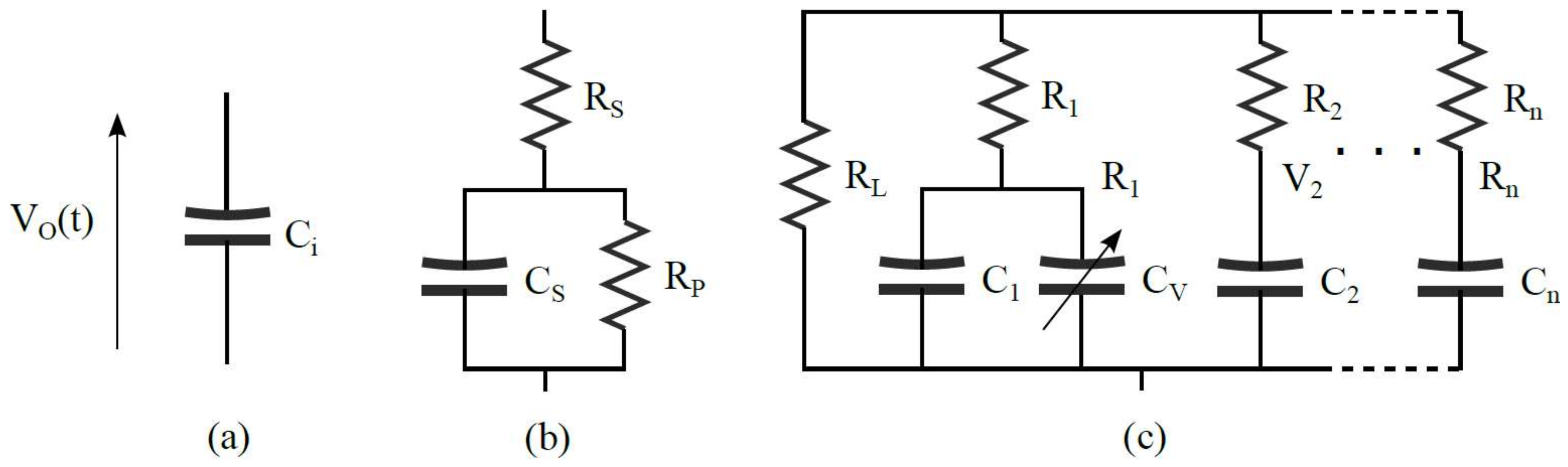
Electronics 07 00044 g001
Figure 2. Circuit-based supercapacitor models: (a) an ideal capacitor. (b) Simplified model including a series and parallel resistance. (c) RC ladder circuit with a voltage-dependent capacitance in its first branch, which may be extended to n branches.
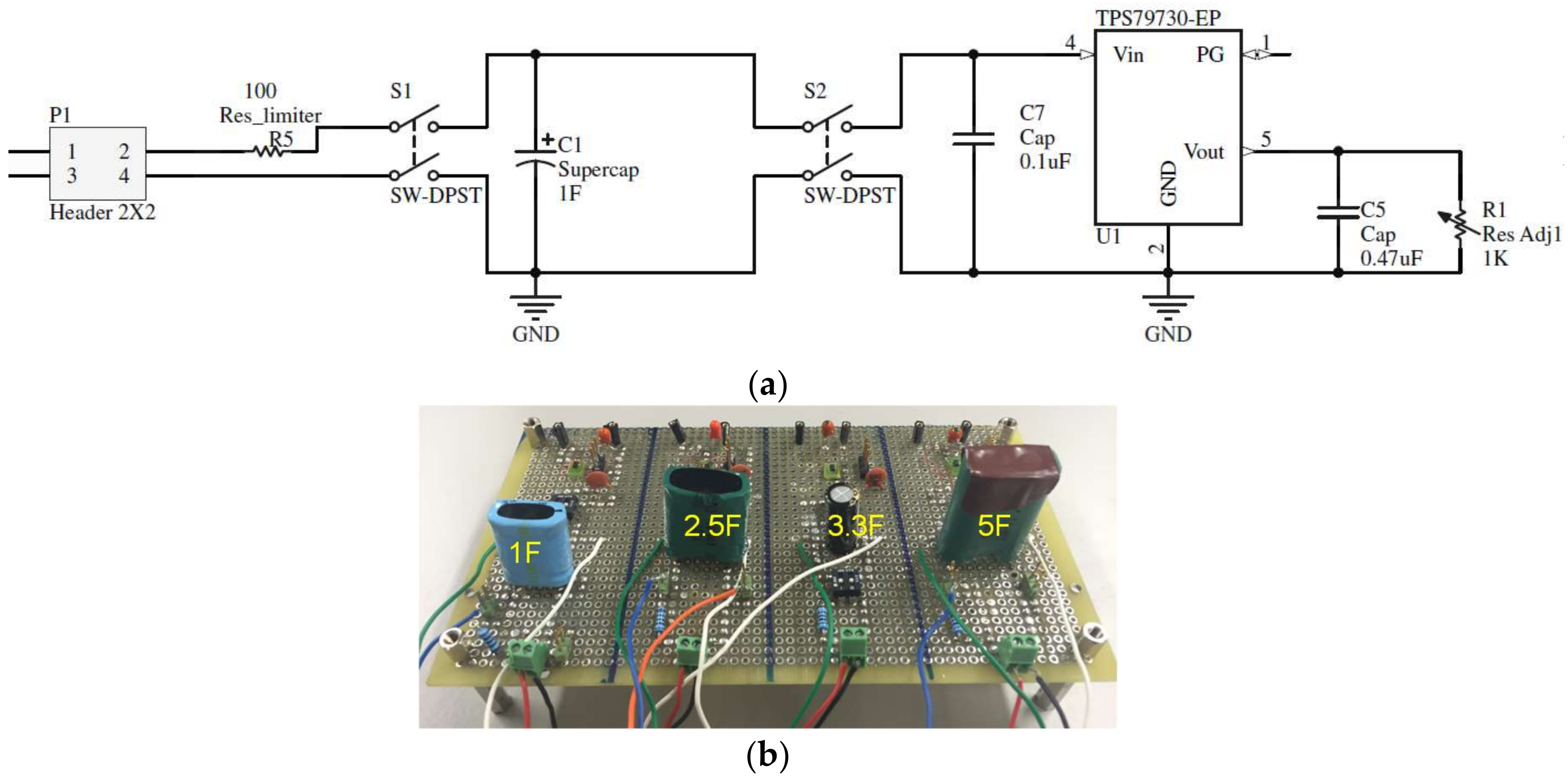
Electronics 07 00044 g002
Figure 3. Evaluation board set-up. (a) Schematic of a single capacitor test fixture. (b) Complete test evaluation board.
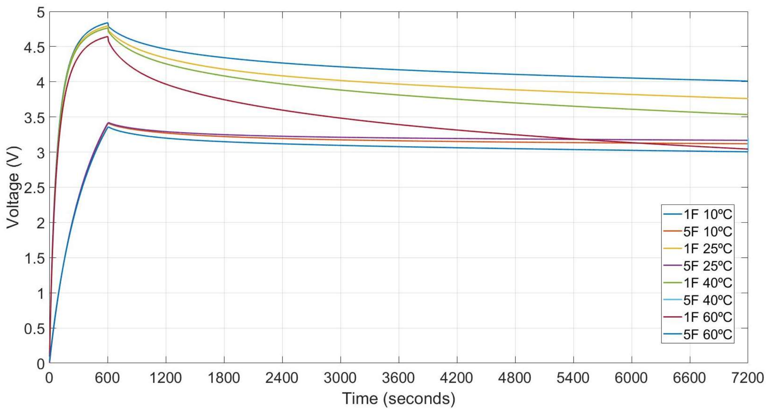
Electronics 07 00044 g003
Figure 4. Charge and discharge profiles at 10, 25, 40 and 60 °C for supercapacitors of 1 and 5 F.
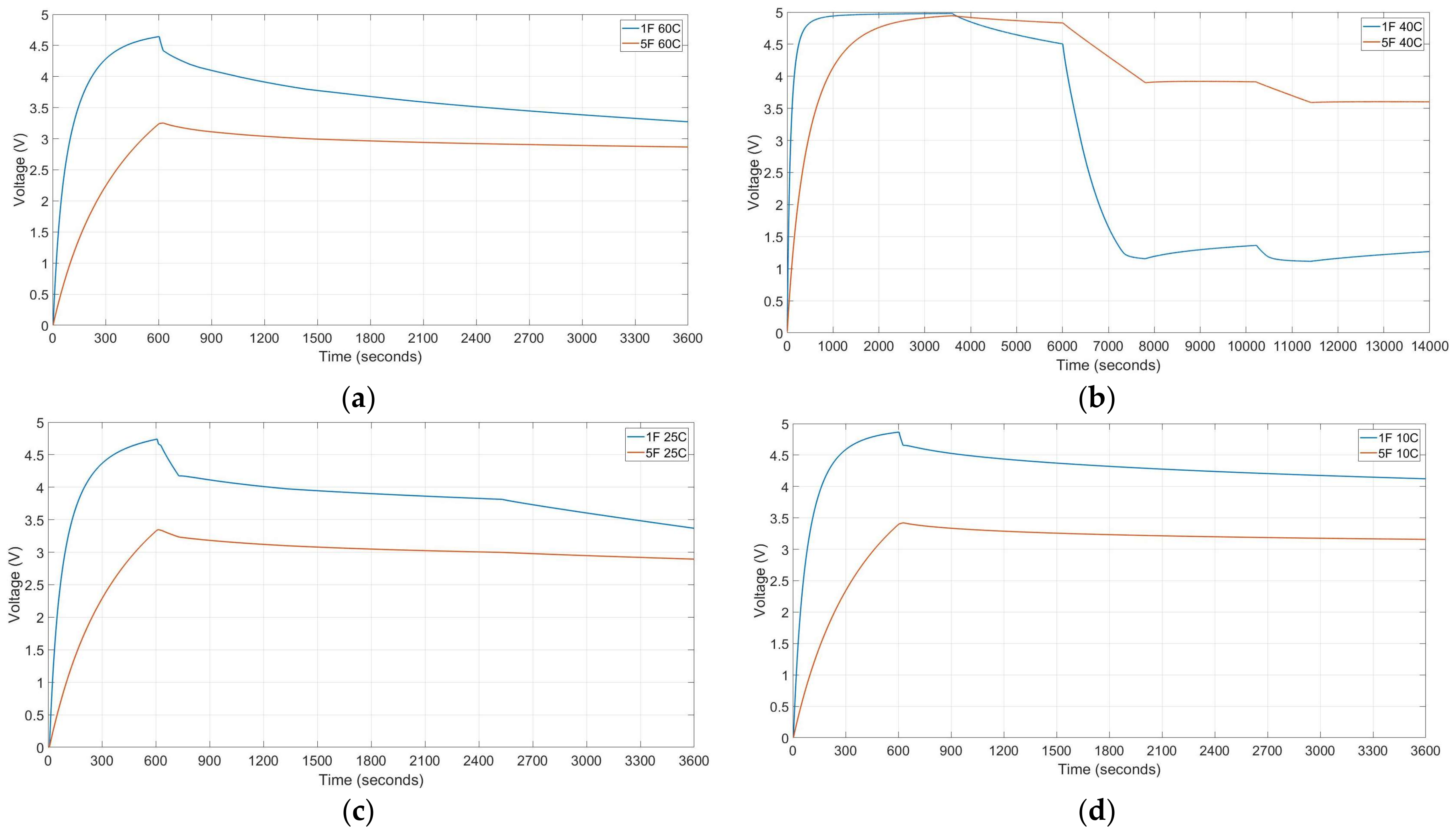
Electronics 07 00044 g004
Figure 5. Charge and discharge profiles of 1 and 5 F supercapacitor at different test conditions. (a) T = 25 °C, tcharge = 600 s, Vcharge = 5 V, discharge profile (5 steps of Ileak 30 s, 3 mA 90 s, 0.058 mA 600 s, Ileak 1200 s and 0.3 mA until discharge). (b) T = 40 °C, tcharge = 3600 s, Vcharge = 5 V, discharge profile (five steps: Ileak 2400 s, 3 mA 1800 s, 0.025 mA 2400 s, 1.5 mA 1200 s, Ileak until discharge). (c) T = 60 °C, tcharge = 600 s, Vcharge = 5 V, discharge profile (3 steps: 0.3 mA 180 s, 0.1 mA 600 s, 0.058 mA until discharge). (d) T = 10 °C, tcharge = 600 s, Vcharge = 5 V, discharge profile (single step: 0.02 mA until discharge).
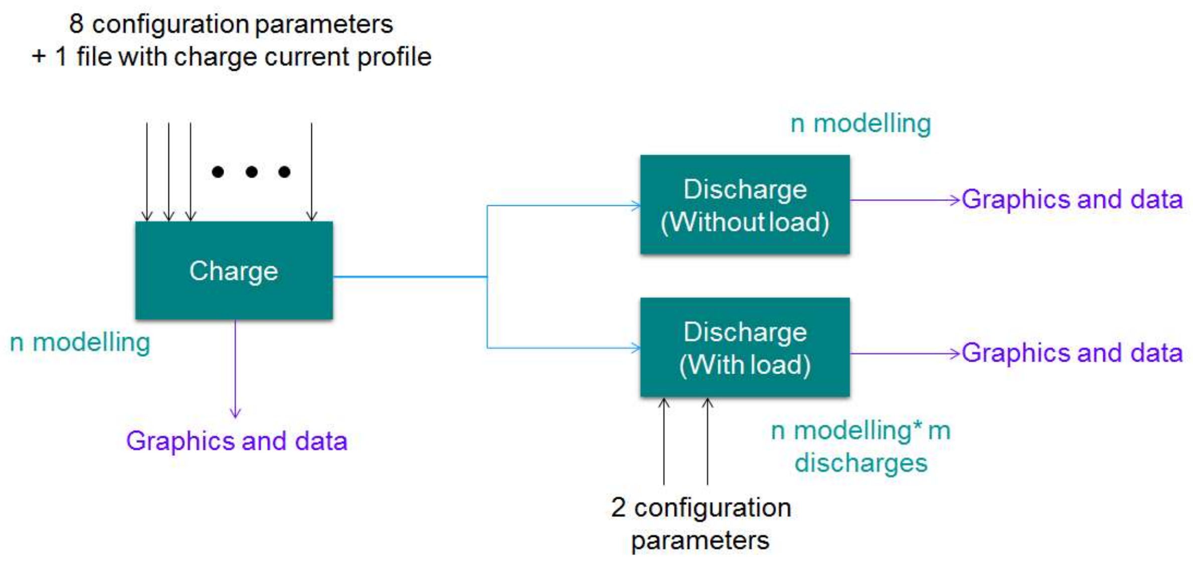
Electronics 07 00044 g005
Figure 6. Model architecture represented as a block diagram, including the program inputs and outputs.
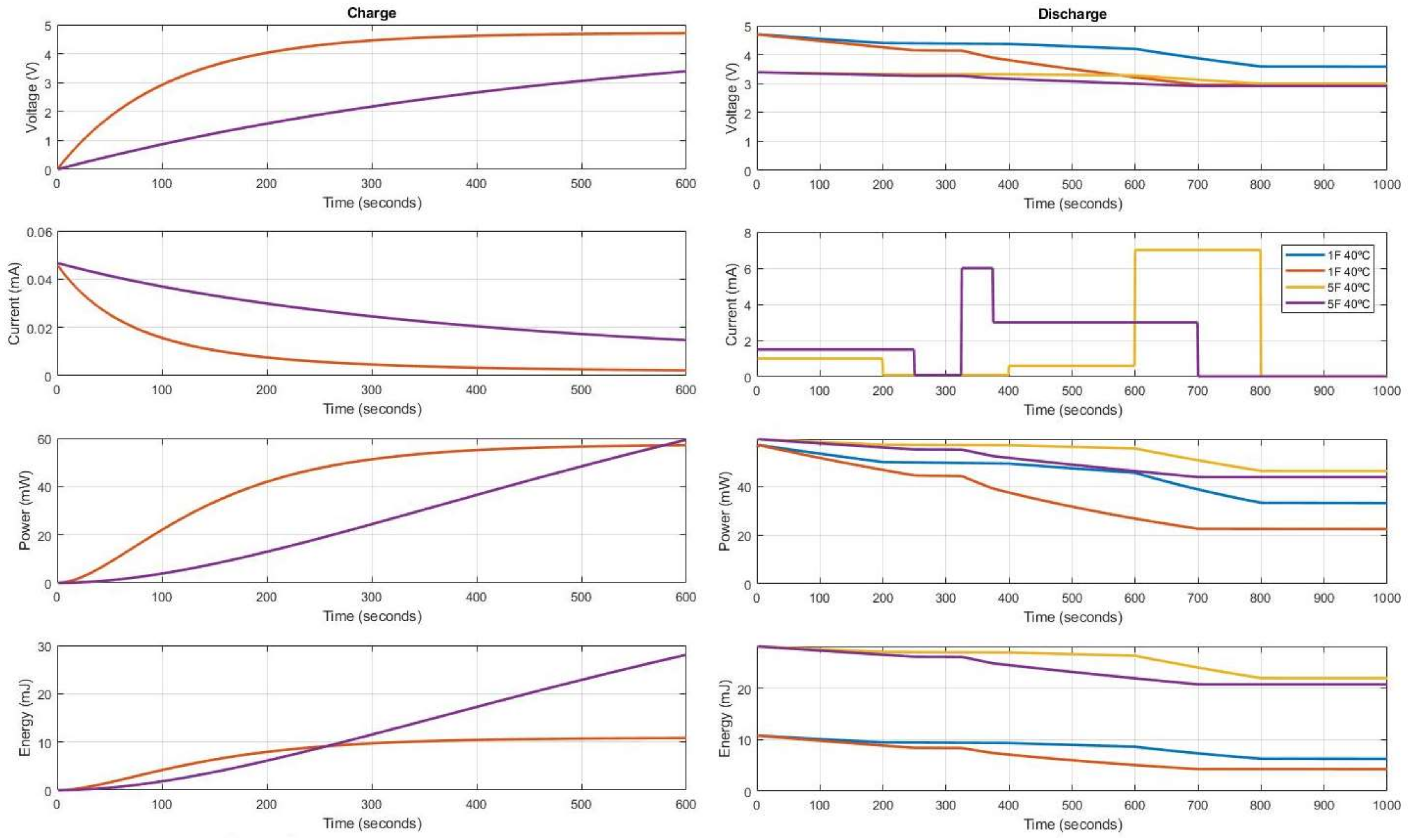
Electronics 07 00044 g006
Figure 7. Mathematical model results with 1 F and 5 F supercapacitors, 600 s charge with 5 V at 40 °C temperature and different profiles of discharge. Yellow discharge profile has five steps all with 200 s of duration; First 1 mA, second self-discharge, third 0.5 mA, fourth 7 mA and fifth self-discharge. Purple discharge profile has also 5 steps; First 1.5 mA for 250 s, second self-discharge for 75 s, third 6 mA for 50 s, fourth 3.5 mA for 325 s and fifth self-discharge for 300 s.
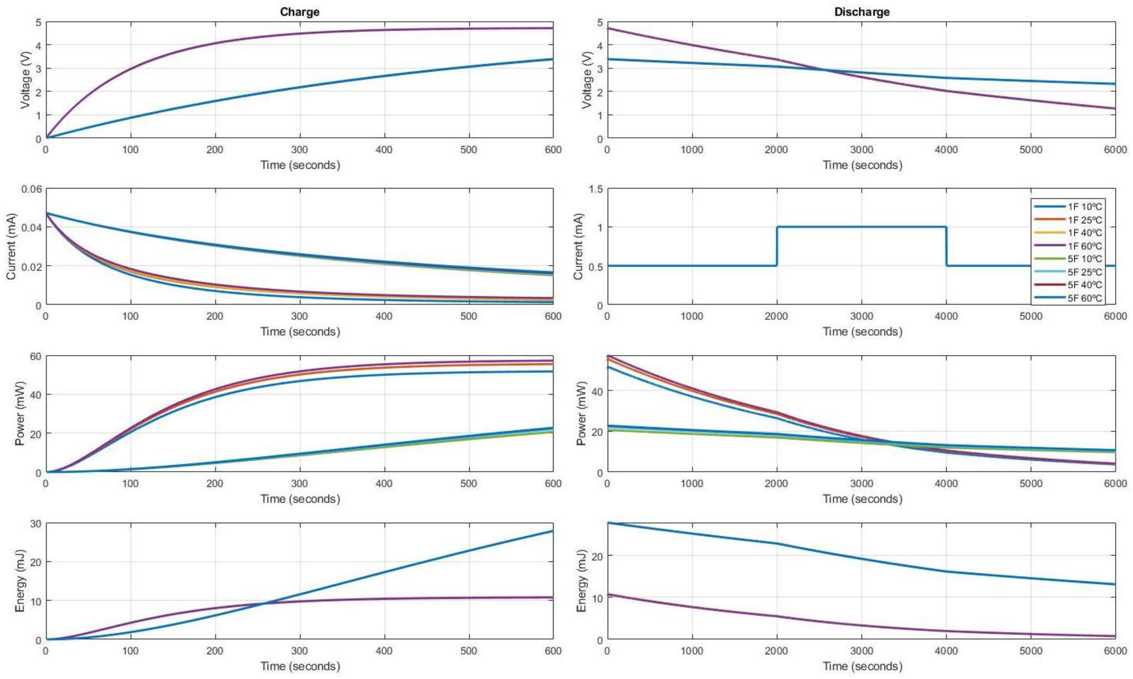
Electronics 07 00044 g007
Figure 8. Charge and discharge results obtained with the mathematical model for 1 F and 5 F supercapacitor values at different temperatures (10, 25, 40 and 60 °C), 600 s charge with 5 V and same outer profile consumption composed by three steps; First step 0.5 mA for 2000 s, second step 1 mA during also 2000 s and third step as first one.
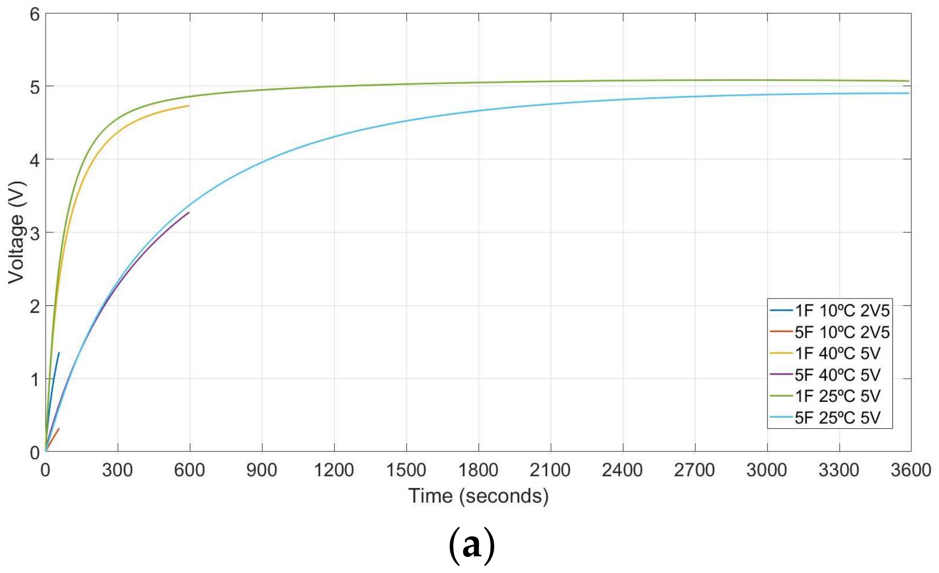
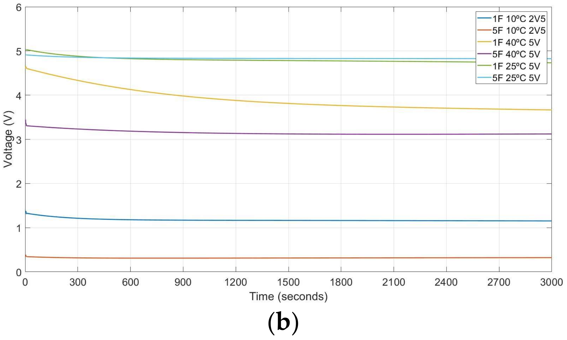
Electronics 07 00044 g008
Figure 9. Obtained results with 3rd approach. (a) Charge curves at different conditions and their (b) self-discharge profiles.
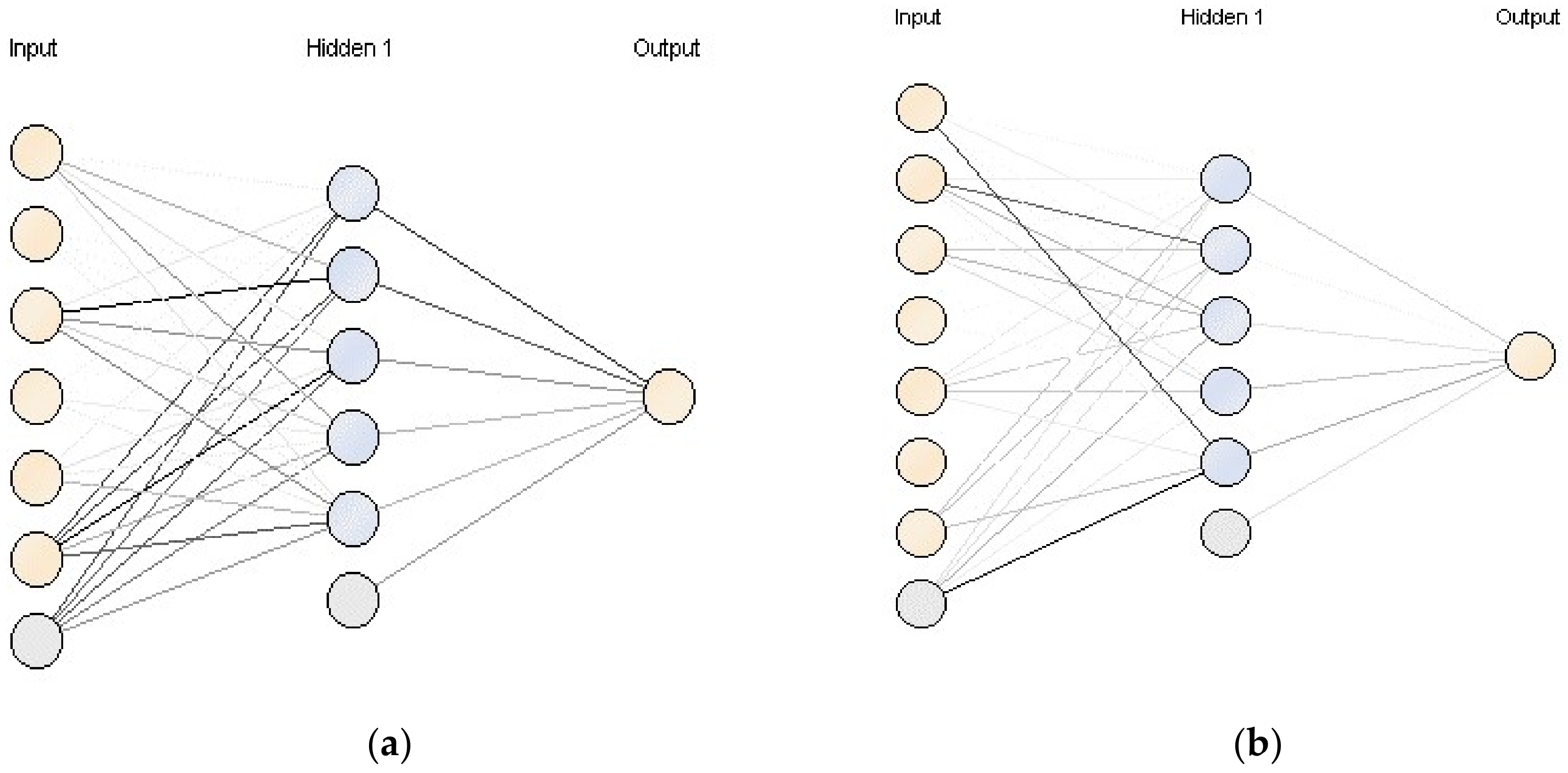
Electronics 07 00044 g009aElectronics 07 00044 g009b
Figure 10. Neuronal networks topologies generated during the experimental analysis. (a) Charge neuronal network topology for all conditions. (b) Discharge neuronal network topology when charge time is 60 s.
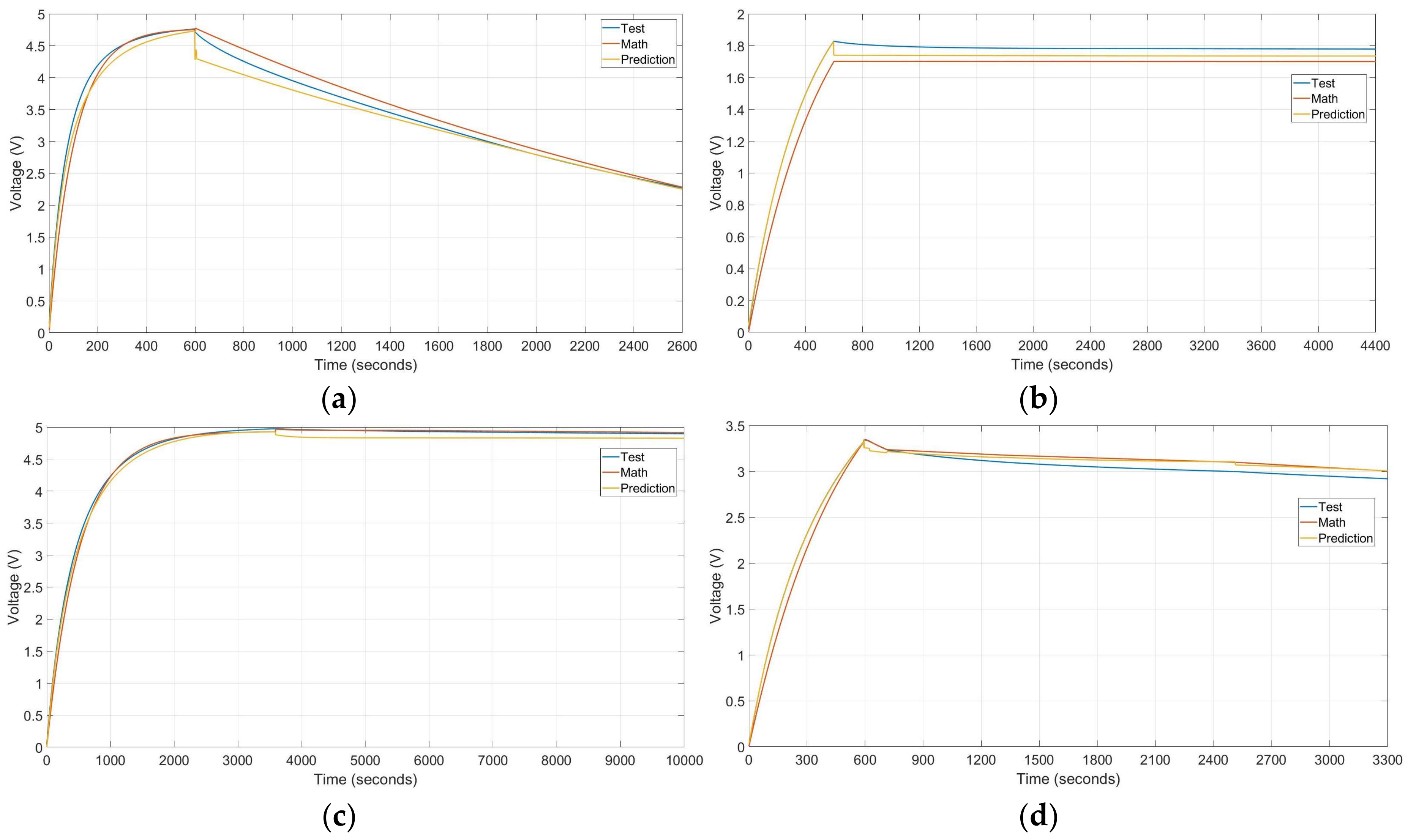
Electronics 07 00044 g010
Figure 11. Graphic results and comparisons of described -four different tests. (a) 1 Farad supercapacitor charged through 10 min with 5 V at 40 °C and 1 mA consumption discharge, (b) 5 Farad supercapacitor charged for 10 min with 2.5 V at 25 °C and self-discharge procedure, (c) 1 Farad supercapacitor charge during 1 h with 5 Volt at 10 °C and self-discharge procedure, (d) 5-Farad supercapacitor charge through 10 min with 5 V at 40 °C temperature and three discharge steps: 0.3 mA consumption through 3 min, 0.1 mA consumption through 10 min and self-discharge.
Electronics 07 00044 g011
Table 1. List of variables and test conditions.
VariableTemperature (°C)Charge Voltage (V)Charge Time (s)Supercapacitor Values (F)Discharge Time (s)
Test conditions10, 25, 40, 602.5, 560, 600, 36001 F, 5 FInfinity load, fixed value load, variable load steps
Table 2. Setting configuration for the MLP network.
ParameterDescriptionValue
hidden_layersName and size of the hidden layers.(number of attributes + number of classes)/2 + 1
training_cylcesNumber of training cycles used for the training phase.500
learning_rateWeight rate change of each step0.3
momentumIt adds a fraction of the previous weight update to the current one.0.2
decayFlag to decrease or not the learning rateFalse
shuffleFlag to shuffle or not the data before learningYes
normalizeThe Neural Net operator uses a usual sigmoid function as the activation function. Therefore, the value range of the attributes should be scaled to −1 and +1. This can be done through the normalize parameter. Normalization is performed before learning. Although it increases runtime, but it is necessary in most casesYes
error_epsilonoptimization training error target value.1 × 10−5
use_local_random_seedFlag to use a random seed for randomizationNo
local_random_seedLocal random seed. It is only used if use_local_random_seed is set to TRUE-
Table 3. Variables used for the development of the prediction models.
VariableData TypeValues
TimeInteger
Temperature (°C)Integer10, 25, 40, 60
Voltage (V)Integer2.5, 5
Charge Time (s)Integer60, 600, 3600
CapacitanceInteger1 F, 5 F
Charge currentReal[0–45] mA
Table 4. Obtained statistical results in different approaches and at different conditions.
VariableData TypeValuesRMSESd
1stChargeFor all conditions of the test0.0070.005
DischargeFor all conditions of the test0.2220.035
2ndDischargeCharge-Time (60)0.0070.002
Charge-Time (600)0.2320.091
Charge-Time (3600)0.1110.024
3rdDischarge and charge curve at the same modelCharge-Time (60)0.0210.002
Charge-Time (600)0.2130.071
Charge-Time (3600)0.2440.098
Table 5. Obtained statistical errors from prediction and electro-mathematical models on three described tests and the average of 36 tests.
Statistical Technique(a) Example(b) Example(c) Example(d) ExampleAverage All
Pred.MathPred.MathPred.MathPred.MathPred.Math.
ChargeRMSE0.1370.2040.1130.1780.0070.1450.0050.1340.0520.146
MSE0.0190.0420.0130.0320.00010.0210.000020.0180.0050.023
MAE0.1230.1250.1030.1670.0060.1140.0040.1180.0470.101
MAPE3.6065.3544.68911.6420.6554.3871.5148.6073.5495.712
DischargeRMSE0.1190.1230.0710.0830.1570.0480.0740.0860.0990.134
MSE0.0140.0150.0050.0070.0250.0020.0050.0070.0170.031
MAE0.0790.1110.0640.0780.1430.0470.0690.0810.0900.128
MAPE2.0133.2102.2112.6533.6591.2302.2722.6852.8193.792
Table 6. Comparison between this work and other model.
Model TypeRef. Numb.Statistical ErrorRef. ResultThis Work Result
Electro-mathematical[12]Deviation3–7%2.35%
Electro-mathematical[34]Deviation2.56%2.35%
Electro-mathematical[35]RMSE0.650.071–0.204
M.L. → ANN[23]MSE0.0890.005–0.017
M.L. → Kalman Filtering[36]MAE0.500.047–0.090
RMSE0.630.052–0.099

