Analysis of Network Attack and Defense Strategies Based on Pareto Optimum

Abstract

Improving network security is a difficult problem that requires balancing several goals, such as defense cost and need for network efficiency, to achieve proper results. Modeling the network as a game and using optimization problems to select the best move in such a game can assist network administrators in determining an ideal defense strategy. However, most approaches for determining optimal game solutions tend to focus on either single objective games or merely scalarize the multiple objectives to a single of objective. In this paper, we devise a method for modeling network attacks in a zero-sum multi-objective game without scalarizing the objectives. We use Pareto Fronts to determine the most harmful attacks and Pareto Optimization to find the best defense against those attacks. By determining the optimal solutions through those means, we allow network administrators to make the final defense decision from a much smaller set of defense options. The included experiment uses minimum distance as selection method and compares the results with a minimax algorithm for the determination of the Nash Equilibrium. The proposed algorithm should help network administrators in search of a hands-on method of improving network security.

1. Introduction

1.1. Introduction

In recent years, study into the economics of information security has become a hotspot for network security research. Indeed, it is now common to compare the costs and benefits of different attack and defense strategies. Stolfo et al. [1] was the first to propose a solution using a cost-sensitive model as the basis for a primary response strategy. The system would compare the cost of defense to the cost suffered by intrusion and if the response cost exceeded the intrusion cost, the system would take no action.

This concept of intrusion cost has spread through the field of computer risk assessment and quantitative cost assessment has become a foundation for work in the field. At the same time, there are some shortcomings: (1) not all problems can be properly quantified, i.e., in some cases, cost classification is possible, but not quantification; and (2) quantitative cost estimation is well suited for intrusion detection systems (IDS), but underperforms when choosing a defense strategy.

1.2. Related Works

Bistarelli and others [2] attempted to assuage this problem by proposing an evaluation approach that uses both qualitative and a quantitative return on investment (ROI) rather than just cost. The ROI approach allows a security administrator to determine whether a defense strategy is worth the cost.

Using empirical evidence, Gordon et al. [3] studied budgeting and economic activities of computer safety companies. The results show that safety factors, such as the cost–benefit analysis, began to be considered by safety management personnel for expenditure budget and security decision-making [4]. Feng [5] proposed a cost estimation model using vulnerability. Using an active and comprehensive vulnerability analysis, he calculated the reliability of the system and the cost of an attack. The defending administrator can use this as a reference to compare the cost of defense to that of repairing the system.

The elements and characteristics of the network attack and defense model are consistent with the definition, elements and characteristics of game theory [6]. The interaction between the attacker and the defender conforms to player interaction in the game theory. Game theory provides us with a mathematical framework to solve the network security analysis and modeling helps us understand attacker behavior and select an optimal defense strategy for security protection. Carin [7] proposed a method for quantifying network security risk for security policy effectiveness and analyzed key infrastructure protection strategies using attack and defense models. Lye and Wings [8] used a stochastic game model to determine a Nash Equilibrium for the defender and attacker and their respective optimal strategies [9]. A Nash Equilibrium is a solution of a game where none of the players are sufficiently incentivized to change strategy. Simply put, it is a state in which each player will keep doing what it was doing at that point [10].

From the inception of computer network, researchers have been focusing on network security. Emergence of Internet based services has opened new doors for hacker to exploit network security. Several types of malicious software have been widely studied by researchers, such viruses, worms, botnets, etc. Among other types of Malware attacks, computer worms are well-known for its capability to bring down a network, even Internet. Most notable feature of worms are its small size and fast infections spread capability, since worms do not require human to propagate through the network. Slammer worm, which is the fastest know worm [11], took only 10 min to reach its targets. The severity of attack by worm depends on scanning rate, infection topology and intended attack on target.

Unlike worms, a virus propagates by replicating itself and requires an executable host file. It often resides in USB flash disks and files transmitted via email. Trojan is another category of malware that tries to run as a legitimate software. Since our model considers a static form of attack and defense, it can only be used to design worm like attack considering possible attack and defense scenarios.

Since the first well-known DDOS attack against Minnesota University in 1999 [12], the methods and tools used in the attacks have changed significantly. The two general types of DDOS attacks are: (1) bandwidth depletion attacks involving flooding or amplification of network traffics (e.g., flooding, ping of death); and (2) resource depletion attacks involving sending malformed packets or misuse of a protocol to bring down a resource [13] (e.g., TCP SYN flooding, IP address attacks).

Due to the explosive grow of the Internet of Things, the botnet army attack, which uses IOT-based botnets has emerged, as a new form of DDOS attack [14]. Since most of the devices connected to IoT networks are controlled by C&C units with little or no authentication, they are often conscripted into botnet armies. The DDoS attacks on KrebsOnSecurity and Dyn by Mirai malware are the largest by data, and are responsible for conscripting at least 500,000 IoT devices in 164 countries [15]. Another interesting form of DDOS attack that emerged recently is booters (sometimes referred as stresses) in which attack is provided as-a-service [16]. Using a misconfigured DNS for amplification is a popular technique used by booters [17].

DDOS attacks over Tor network became popular in 2013 after Dannis Brown’s presentation at Defcon18, on using Tor network to provide anonymity for C&C server. However, this method is not as stealthy as it claims to be, since bots using Tor are detectable due to the characteristic in their network traffic [18].

The malicious attack described in our model closely resembles botnets. Botnets are used to perform automated tasks and were first used in IRC channels to implement centralized command and control (C&C) [19]. Since bots can be remotely controlled, they are often used in DDOS attacks [20]. Dainotti et al. analyzed horizontals scanning IPv4 address space employed by the Sality botnet. They emphasized the difficulty of detecting the new-generation of Botnets and proposed a visualization technique to explore botnet scan propagation. The simulator we developed lacks this capability since our primary focus of the visualizing aspect of the application was visualizing the defense and attack strategies of the network.

Dainotti et al. proposed a mechanism for DDOS detection based on Continuous Wavelet Transform [21]. Unlike their system, our system is focuses on the strategy calculated based on the resources available to the administrator and his/her priority.

Recently, Abshof et al. [22] analyzed dynamics in multi-level networks. Although the static representation of the network and cost calculation are similar to the one in our model, their model focuses on measuring the quality of Nash Equilibria. In a review article, Liang [23] explored the overall research process in cyber security and provided us with a variety of game theory application, each adapted to different security scenarios.

At present, there are three main problems in using traditional game models to determine an optimal defense strategy: (1) the final optimal defense strategy is generally a combination of game theory results and optimization by the security manager; (2) network availability is often weakened by cost and benefit tradeoffs, despite a general need for information networks to prioritize availability; and (3) powerful analysis methods such as Bayesian equilibrium, Markov decision process and de-fuzzification, which are used in many related studies, are difficult to calculate and low in efficiency [24].

Whilst this paper does not solve all the problems associated with network defense game models, it does present us with specific approach to aid security managers in choosing an optimal solution. In previous research [25,26], we have studied the dynamic game process between attackers and defenders. This paper focuses on analyzing the static interaction process in each game, aiming to show that using Pareto Optimization allows security managers to make this choice without actually knowing the attackers exact move.

In very simple terms, Pareto Optimization can be described as the removal of objectively inferior solutions from a solution set. The removal of these objectively inferior solutions means that the security manager is confronted with a smaller set of available options, simplifying the subjective phase of defense strategy selection. The model also gives us a starting point for dynamic goal distribution. Pareto Optimization allows us to define a targeted goal distribution (“network availability/cost” ratio) and choose an optimal decision for that distribution.

The approach allows us to choose an optimal solution for a single attacker defender interaction. This can be done subjectively by the defender or by means of a ranking algorithm. Eventually, this approach will be incorporated into an interactive game with multiple interactions.

It is good to contrast our approach with similar research. Wu et al. [27] conducted an experiment based on game theory to tackle Denial of Service (DOS) and Distributed Denial of Service (DDOS). They have covered both static and dynamic game scenarios for DDOS. Although their model is very similar in many aspects, the major differences are the topology and objective of the players. In the game model proposed by our work, the players (both attacker and defender) have multiple objectives. In contrast to Wu et al. model, we modeled our network as a peer-to-peer network. In addition to that, in our model, the attacker does not have specific target service provider, since one of the goal is to bring down over all network availability. Studer and Perrig [28] studied a similar attack pattern to DDOS, called Coremelt attack. The botnets participating in the Coremelt attack floods the network by sending all the other peers in the network. The authors of Coremelt only focused on proving the success of the attack, not the preventive mechanism.

One disadvantage of the Pareto Optimization approach is that it is less efficient than alternative solutions to zero-sum games. The best-case complexity is O(n × log(n)) and the worst-case complexity is O(m(n)²). By contrast, a basic minimax approach would be more efficient at a worst case of O(m × n).

This paper focuses on determining optimal defense and attack strategies for a multi-objective zero-sum game representation of an attack on a computer network. The study limits itself to computer networks that consist of a fixed number of devices (Servers, clients, routers, etc.) connected as a complete graph. The players of the game have several zero-sum objectives, allowing for the use of Pareto Optimization in determining the best strategies for the players [29].

1.3. Article Structure

This paper briefly describes a conceptual model and implementation for applying Pareto Optimization to multi-objective network defense. The model was implemented and simulated in our custom coded Pareto Defense Strategy Selection Simulator (PDSSS). Section 2 describes in detail the model used to simulate a network and the corresponding attack on the network. Section 3 shows the core implementation of the model in the PDSSS. Section 4 shows the results of a complete simulation and the interpretation of the results. Finally, Section 5 discusses our concluding thoughts and ideas for future work.

2. Game Model Based on Pareto Optimum

The significance of this paper lies in proposing a novel attack–defense game based on failure rate, mean time to repair and network availability loss. The proposed game solution attempts to identify and remove objectively inferior strategies before determining an optimal defense strategy. The paper includes a description of our implementation and an experiment to validate the optimization model.

The game is defined as:

$$Game=(G, P, S_{attack},S_{defense},F)$$

(1)

where G is the graph representation of the computer network, P is the set of players, S_attack is the set of possible attack strategies, S_defense is the set of possible defense strategies, and F is the payout matrix for the game.

2.1. Network Definition

G is a graph representation of a computer network where the vertices represent the devices and the edges represent connections between the devices.

$$G=(V,E)$$

(2)

2.1.1. Vertices Definition

Vertices are all the device connected to the network that can be part of an attack chain. Each of these devices has a set of device attributes. For the sake of simplicity, we limit ourselves to just two types of devices, servers and client machines. The total number of vertices is then the sum of the total number of servers and client machines.

We define three device attributes, capture cost (cc), available connections (conn) and access (access). The capture cost is the cost associated with compromising a device, effectively replacing it with a malicious insider from which the attacker can launch a new attack [30]. The two possible devices give us two possible values for the capture cost attribute namely: $c_{server}$, the capture cost for a server and $c_{client}$, the capture cost for a client machine. The available connections are the number of connections that the vertex can be accessed by. The available connections range between 0 and a network maximum of SC. The access attribute defines whether a vertex can be captured by an attacker. This is either true or false.

$$V=\left\{v_1,\dots ,v_n\right\}$$

(3)

The total number of vertices is n. A single vertex v has the device attributes:

$$v=cc,conn,access|cc\in \left\{c_{client},c_{server}\right\},conn\in \left[0,SC\right],access\in \left\{0,1\right\}$$

(4)

where SC is the maximum number of connections that a defender can allocate to a vertex.

2.1.2. Edges Definition

Edges are the links between the devices. For simplicity, we assume that the network is a simple undirected graph where each vertex is connected to each other vertex by a single edge. Here, (i,j) represents a link between i and j, where the i and j are vertices in the graph. Note that vertices can only have one link between them, thus (i,j) refers to the same as link as (j,i).

$$E=\{(i,j) | i,j \in V, i \ne j\}$$

(5)

Each of the edges has a set of edge attributes. We have given the link just two attributes, namely the number of shared connections (sc) on the link and the link fail rate (lfr). The attributes for the link (i,j) have the following characteristics:

$$sc(i,j)=\min \left\{conn(i),conn(j)\right\}, 0\le lfr(i,j)\le 1$$

(6)

Note the intended interpretation that if one of the vertices has no shared connections, sc(i,j) = 0, no traffic can flow to that vertex and the link is effectively down.

The more connections are available on a single edge, the greater is the bandwidth of the network channel. However, many open connections expose the network to outside threats. An example of this is the 2017 NotPetya malware attack, which worked by accessing a device using ports 137, 138, 139 and 445 [31]. Network administrators could defend themselves from by blocking access to these ports, among other things. This shows that closing shared connections will increase security of the network. In our example, a vertex where all links have ports 137, 138, 139 and 445 closed, would have its access = 0 for the NotPetya attack. A vertex with those ports open, would have access = 1.

The link fail rate is the likelihood that the link will fail at any given point. To calculate the lfr, we need to determine two variables. First, the mean time between failures (MBTF) of the link. MBTF(i,j) is the average time it takes a link to fail after the last repair. The longer MBTF(i,j), the higher the reliability of the link. Next, we need the mean time to repair (MTTR) of the link. MTTR(i,j) is the average time between repairs for the link. The shorter the MTTR(i,j), the less likely it will be down at a given point. Using these two values, we can calculate the link fail rate which gives us a ratio indicating how likely it is for the link to fail.

$$lfr(i,j)=\frac{MTTR(i,j)}{MTTR(i,j)+MTBF(i,j)}$$

(7)

2.2. Players and Strategies

The players in the game can be either attackers or defenders. Every game should have at least one attacker and one defender. Attackers can only use attack strategies (s_attack ∈ S_attack) and defenders can only use defense strategies (s_defense ∈ S_defense). The game is an incomplete information game, i.e., the players do not know each other strategy. The game discussed in this scenario assumes a total of two player.

$$P=\left\{attacker, defender\right\}$$

(8)

2.2.1. Defender’s Strategies

Defenders protect the network by either increasing or decreasing the number of shared connections on a network edge. As previously noted, a greater number of connections increase network performance, while fewer connection increase network security in the cost of low network performance. The defender can decrease the number of connections on a link by changing the number of available connections in one or both devices connected by the link. By playing with the number of available connections, the shared connections on a link can be changed to any between zero and the maximum number of available connections, SC. The number of connections in a link can be described as:

$$s{c}_D(i,j)=s{c}_0(i,j)+s{c}_d(i,j) \in \left[0,\mathrm{SC}\right]$$

(9)

where $s{c}_D(i,j)$ is the total number of shared connections on the link $(i,j)$ after implementation of the defense strategy; $s{c}_d(i,j)$ is the change in number of connections on the link $(i,j)$ by the defense strategy and $s{c}_0(i,j)$ is the number of shared connections at the start of the game. Note that $s{c}_D(i,j)$ cannot exceed the number available connections of either vertex.

The defender can choose a defense strategy from a predetermined set of defense strategies:

$$S_{defense}=\left\{s_{defense}^{(1)},\dots ,s_{defense}^{(d)},\dots ,s_{defense}^{(D)}\right\}$$

(10)

where D is the total number of available defense strategies and a single defense strategy is defined as a vector containing the resulting change in number of connections for each link:

$$s_{defense}=s{c}_d(1,2),\dots ,s{c}_d(i,j),\dots ,s{c}_d(n-1,n) | (i,j)\in E$$

(11)

2.2.2. Attacker’s Strategies

Attackers can attack the network using attack chains. An attack chain is a sequence of connected vertices starting at a captured vertex and ending at any other vertex in the graph. The attack chain will traverse an edge only once and “attack” every edge it traverses.

An attack consists of two steps. First, we need to capture one or more vulnerable devices (i.e., a vertex with access = 1) to gain access to the network. We can represent this step with a vector, q, containing all the vertices and whether the vertex is captured by the attacker. This is either true or false, i.e., 0 or 1. Note that the attacker can only capture vertices with access = 1. Assuming an attack on a network with n vertices, we get:

$$q=\left[q_1,\dots ,q_i,\dots ,q_n\right] | q \in {\left\{0,1\right\}}^n$$

(12)

Then, the attacker uses that vertex as a starting point for an attack chain. Note that once the attacker captures a vulnerable vertex, it effectively gains access to every other vertex, because our network is a complete graph. We can write a sequence with length l as:

$$chain=v^{(1)}\to v^{(2)}\to \dots \to v^{(l)} | v \in V$$

(13)

To lower network availability, an attack on an edge means that it will attempt decrease the number of available shared connections in the edge by $s{c}_{attempt}$ which cannot exceed the network specified maximum number available connections, SC.

$$\begin{gathered} attackchain=(chain, s{c}_{attempt}) \\ chain \in {\left\{V\right\}}^l | 1 \le l\le n and 0\le s{c}_{attempt}\le SC \end{gathered}$$

(14)

Not every attempt on an edge will be successful. In fact, the actual number of shared connections that the attacker can decrease a link is limited by a basic bottleneck. An attack chain cannot decrease the number of shared connections by less than then smallest number of available connections on any given edge in the chain. We can describe this actual decrease in the number of shared connections as:

$$\begin{gathered} s{c}_a=\min \left\{s{c}_{attempt},bottleneck(chain)\right\} \\ bottleneck(chain)= \min \left\{s{c}_D(v^{(1)},v^{(2)}), s{c}_D(v^{(2)},v^{(3)}), \dots , s{c}_D(v^{(l-1)},v^{(l)})\right\} \end{gathered}$$

(15)

The result of the attack chain will be that every edge in the chain will have the number of shared connections reduced to:

$$sc(i,j)= s{c}_D(i,j)- s{c}_a | i,j\in chain$$

(16)

A single attack strategy consists of implementing every attack chain a defined set of attack chains. A single attack with M attack chains is defined as:

$$s_{attack}= q, \left\{attackchai{n}_1,\dots ,attackchai{n}_M\right\}$$

(17)

The attacker can choose an attack strategy from a predetermined set of attack strategies:

$$S_{attack}=\left\{s_{attack}^{(1)},\dots ,s_{atack}^{(a)},\dots ,s_{attack}^{(A)}\right\}$$

(18)

where A is the total number of available attack strategies.

2.3. Goals of Game

This is a multi-objective zero-sum game. The fact that it is multi-objective means that there are multiple payment functions. The fact that it has zero-sum means that objectives of the player are diametrically opposed. If the goal of one player is to maximize a payment function, the goal of the other player is to minimize that function, and vice-versa. The resulting payment function and objectives for a single game are:

$$F(s_{attack}^a,s_{defense}^d)= {\overline{f}}_{a,d}=\left[f_{a,d}^{(1)},f_{a,d}^{(2)},\dots ,f_{a,d}^{(K)} \right]$$

(19)

$$min/\max F(s_{attack}^a,s_{defense}^d)$$

(20)

where K is the total number of payment functions. For simplicity, we have limited ourselves to two payment functions, K = 2. The first is to minimize (for the defender) or maximize (for the attacker) the change in network failure. The second is to minimize (for the defender) or maximize (for the attacker) cost difference between defense and attack strategies.

2.3.1. Network Failure Rate

As payment function for the network failure, we can use the change average fail rate (AFR) of the network. We can calculate the average fail rate at a given time t, by taking the fail rate of each link and multiplying it by the number of shared connections on that link. If one averages that over the total number of shared connections in the network, it will give you the average fail rate (AFR) of the network.

$$AFR(t)=\frac{{{\displaystyle \sum }}_{i=1}^{n-1}{{\displaystyle \sum }}_{j=i+1}^{n}sc(i,j)\ast lfr(i,j)}{{{\displaystyle \sum }}_{i=1}^{n-1}{{\displaystyle \sum }}_{j=i+1}^{n}sc(i,j)}$$

(21)

where sc(i,j) is the number of shared connections at time t. The initial fail rate, is:

$$AFR(0)=\frac{{{\displaystyle \sum }}_{i=1}^{n-1}{{\displaystyle \sum }}_{j=i+1}^{n}s{c}_0(i,j)\ast lfr(i,j)}{{{\displaystyle \sum }}_{i=1}^{n-1}{{\displaystyle \sum }}_{j=i+1}^{n}s{c}_0(i,j)}$$

(22)

Our game consists of a single round. Hence, we can assume that the game starts at t = 0 and by t = 1 both attacker and defender will have implemented their strategies. The change in average AFR is thus AFR(1) − AFR(0). We can normalize using AFR(0) to get the first payment function:

$$f_{a,d}^{(1)}=\frac{AFR(1)-AFR(0)}{AFR(0)}$$

(23)

The defender’s goal is to minimize f_a,d⁽¹⁾ and the attacker’s goal is to maximize f_a,d⁽¹⁾.

2.3.2. Cost of Defender and Attacker

As payment function for the cost, we can use the difference between the cost of implementing a defense strategy and the cost of implementing an attack strategy.

The cost of a defense strategy lies in adjusting the number of shared connections. If we assume a fixed cost for the change in a single shared connection, we can easily calculate the cost of the defense strategy. Using the defense strategy definition in Formula (11), we get the following cost for a defense strategy:

$$cost(s_{defense})={\displaystyle \sum }_{i=1}^{n-1}{\displaystyle \sum }_{j=i+1}^{n}cos{t}_{adjust}(i,j),cos{t}_{adjust}(i,j)= \alpha ·\left|s{c}_d(i,j)\right|$$

(24)

Here, cost_adjust is the cost of adjusting link (i,j); α is the cost of adjusting a single shared connection and |sc_d(i,j)| is number of adjusted connections (either opened or closed).

The cost of an attack strategy consists of two parts. The first part is the cost of capturing vulnerable vertices. The second part is the cost of occupying the shared connections between the vertices. The attacker must pay a cost for every shared connection it attempts to occupy. This is despite the fact that the actual number of occupied shared connections can be less than sc_attempt due to the bottleneck effect described in Formula (15). Using the attack strategy definition in Formula (17), we get the following cost for an attack strategy:

$$\begin{gathered} cost(s_{attack})= cos{t}_{capture}+{\displaystyle \sum }_{m=1}^{M}cos{t}_{occupy}(attackchai{n}_m) \\ cos{t}_{capture}= {\displaystyle \sum }_{i=1}^n(q_i\ast cc(v_i)) | v_i\in V \\ cos{t}_{occupy}(attackchai{n}_m)= \beta ·(l^{(m)}-1)·|s{c}_{attempt}^{(m)}| \end{gathered}$$

(25)

Here, $cos{t}_{capture}$ is the cost of capturing the vulnerable vertices, $q_i$ is whether the vertex is captured, and $cc(v_i)$ is the capture cost as defined in Formula (25). The cost for occupying the connections is given by $cos{t}_{capture}$ and uses $\beta$ as the cost for attempting to occupy a single connection, $l^{(m)}$ is the length of $attackchai{n}_m$ and $|s{c}_{attempt}^{(m)}|$ is the number shared connections the attacker is trying to occupy.

Using the above costs, we can calculate the second payment function:

$$f_{a,d}^{(2)}=cost(s_{defense}^{(d)})-cost (s_{attack}^{(a)})$$

(26)

The defender’s goal is to minimize $f_{a,d}^{(2)}$ and the attacker’s goal is to maximize $f_{a,d}^{(2)}$.

2.4. Pareto Optimization

This paper uses Pareto Optimization to find the optimal strategy. First, we need to define Pareto dominance and the Pareto front.

Pareto Optimization is a technique used to find optimal solutions in multi-objective optimization problems. The idea here is that some solutions are objectively inferior to others. If we remove the objectively inferior solutions from a function image, the remaining solutions give a smaller set of solutions to choose the optimal solution from. To find this, we introduce the concept of Pareto dominance. A solution that is dominated is objectively inferior.

Pareto vector dominance describes a situation where for a vector x and a vector y in the same solution space, vector x is said to dominate vector y, if and only if x is superior to y in every function in the solution space. In the context of a maximization function, superior means greater or equal to, while for minimization function, superior means less than or equal to [32].

For example, imagine having to choose the optimal minimization solution from these three possible solutions (1,4), (7,1), (5,5). The solution (1,4) is superior to (5,5) in all the dimensions of the solution space, i.e., 1 < 5 and 4 < 5. Hence, (1,4) dominates (5,5). However, the same cannot be said for (1,4) and (7,1). This is even though 1 < 4, 7 > 1. Hence, (1,4) does not dominate (7,1).

Using the payment functions from Formulas (23) and (25), we can describe Pareto dominance for minimization as:

$${\overline{f}}_{a,d}\preccurlyeq {\overline{f}}_{a^{\prime },d}≔\forall k\in \left\{1,\dots ,K\right\}, f_{a,d}^{(k)}\le f_{a^{\prime },d}^{(k)}\wedge \exists k\in \left\{1,\dots ,K\right\} : f_{a,d}^{(k)}<f_{a^{\prime },d}^{(k)}$$

(27)

Likewise, for maximization, we can use:

$${\overline{f}}_{a,d}\succcurlyeq {\overline{f}}_{a^{\prime },d}≔\forall k\in \left\{1,\dots ,K\right\}, f_{a,d}^{(k)}\ge f_{a^{\prime },d}^{(k)}\wedge \exists k\in \left\{1,\dots ,K\right\} : f_{a,d}^{(k)}>f_{a^{\prime },d}^{(k)}$$

(28)

Pareto set dominance describes a situation where for a set X and a set Y, X is said to dominate Y, if and only if X contains a vector x that dominates all vectors in set Y. Using the payment functions from Formula (19), we can describe Pareto set dominance for minimization as:

$$F_{s_{defense}^d}\preccurlyeq F_{s_{defense}^{d^{\prime }}}≔ \forall {\overline{f}}_{a^{\prime },d^{\prime }}\in F_{s_{defense}^{d^{\prime }}}, \exists {\overline{f}}_{a,d}\in F_{s_{defense}^d}: {\overline{f}}_{a,d}\preccurlyeq {\overline{f}}_{a^{\prime },d^{\prime }}$$

(29)

The Pareto front is the subset of the solution space, containing only solutions that are not dominated by any other solution. This represents the set of optimal solutions for this optimization problem. Specifically, for minimization, we can use:

$$F_{s_{attack}^a}^{\ast }=\left\{\begin{array}{c}{\overline{f}}_{a,d}\in F_{s_{attack}^a}|\\ \neg \exists {\overline{f}}_{a,d^{\prime }}\in F_{s_{attack}^a}:{\overline{f}}_{a,d^{\prime }}\preccurlyeq {\overline{f}}_{a,d}\end{array}\right\}$$

(30)

Likewise, for maximization we can use:

$$F_{s_{defense}^d}^{\ast }=\left\{\begin{array}{c}{\overline{f}}_{a,d}\in F_{s_{defense}^d}|\\ \neg \exists {\overline{f}}_{a^{\prime },d}\in F_{s_{defense}^d}:{\overline{f}}_{a^{\prime }, d}\preccurlyeq {\overline{f}}_{a,d}\end{array}\right\}$$

(31)

Note that Formula (30) describes a defender trying to minimize against a known attack strategy, while Formula (31) describes an attacker trying to maximize against a known defense strategy.

2.5. Defender Optimization

The defender defends himself in an information incomplete game and thus needs to choose a strategy without knowing what the attacker’s strategy is. Preparing for the worst, the defender should assume that the attacker’s strategy lies on the Pareto front for his defense. By comparing those Pareto fronts, the defender can limit himself to non-dominated defense strategies. The defender can then rank those strategies and choose an optimal strategy. The approach can be explained in a three-step process.

Step 1. Find the attacker’s Pareto front for each defense strategy.

We can use Formula (31) to find the Pareto front for each defense strategy giving us:

$$F_{S_{defense}}^{\ast }=\left\{F_{s_{defense}^1}^{\ast },\dots , F_{s_{defense}^D}^{\ast }\right\}$$

(32)

Step 2. Limit strategies to non-dominated defense strategies

Using Formulas (29) and (32), we can get the set of non-dominated Pareto fronts.

$$F_{s_{defense}}^{ND}=\left\{\begin{array}{c}{F}_{s_{defense}^d}^{\ast }\in F_{S_{defense}}^{\ast }|\neg \exists F_{s_{defense}^{d^{\prime }}}^{\ast }\\ \in F_{S_{defense}}^{\ast }:F_{s_{defense}^{d^{\prime }}}^{\ast }\preccurlyeq F_{s_{defense}^d}^{\ast }\end{array}\right\}$$

(33)

Step 3. Rank and choose an optimal strategy from the remaining set.

To rank the strategies, we determine the distance to the minimum for each Pareto front. The minimum is a point in the target space with the lowest value of the non-dominated Pareto front points in each dimension as its coordinates.

The dimensions of the target space are set by the payment functions. In our implementation, we have two payment functions (f⁽¹⁾ and f⁽²⁾). Therefore, to find the minimum, we need to find the smallest value of each payment function in the non-dominated Pareto fronts.

$${\overline{f}}_{min}=\left[f_{min}^{(1)},f_{min}^{(2)},\dots ,f_{min}^{(K)}\right]$$

(34)

From the non-dominated Pareto fronts, take the lowest value for the necessary payment function.

$$f_{min}^{(k)}=\underset{f_{a,d}^{(k)}\in F_{s_{defense}}^{ND}}{\min }{f}_{a,d}^{(k)}$$

(35)

Note that we can use the same approach to find the maximum. The only difference is that we must find the highest value in the non-dominated Pareto fronts.

To calculate the distance to the minimum of a defense strategy, we can take the average of the distances for each point in the defense strategy.

$$u(s_{defense}^d)=\frac{1}{\left|F_{s_{defense}^d}^{\ast }\right|}{\displaystyle \sum }_{{\overline{f}}_{a,d}\in F_{s_{defense}^d}^{\ast }}\left|{\overline{f}}_{a,d}-{\overline{f}}_{min}\right|$$

(36)

Here, $\left|F_{s_{defense}^d}^{\ast }\right|$ is the number of attack strategies in the given Pareto front.

To properly compare the distances in each dimension, we should normalize the vector. This can best be done by taking the distance to the minimum in each dimension and then dividing it by the maximum range of the dimension (more specifically, the distance between the min and max in that dimension). That should give us:

$$\left|{\overline{f}}_{a,d}-{\overline{f}}_{min}\right|= \sqrt{{\displaystyle \sum }_{k=1}^K{(\frac{f_{a,d}^{(k)}-f_{min}^{(k)}}{f_{max}^{(k)}-f_{min}^{(k)}})}^2}$$

(37)

Here, $f_{a,d}^{(k)}$ is result of the kth payment function for strategies a and d. $f_{min}^{(k)}$ and its compliment $f_{max}^{(k)}$ can be derived using Formula (35). We divide the difference between $f_{a,d}^{(k)}$ and $f_{min}^{(k)}$ by the difference between the min and max in that dimension to get the normalized difference. The rest of Formula (37) is the square root of the summation of the squares, i.e., simple geometric distance. The final distance to the minimum is then:

$$u(s_{defense}^d)=\frac{1}{\left|F_{s_{defense}^d}^{\ast }\right|}{\displaystyle \sum }_{{\overline{f}}_{a,d}\in F_{s_{defense}^d}^{\ast }}\sqrt{{\displaystyle \sum }_{k=1}^K{(\frac{f_{a,d}^{(k)}-f_{min}^{(k)}}{f_{max}^{(k)}-f_{min}^{(k)}})}^2}$$

(38)

We can assume that the defense strategy with the smallest distance to the minimum is optimal.

2.6. Model Limitations

The game model does not represent every possible type of network attack. There have been attempts to model every possible attack that can be made on a network. These attempts tend to focus on either classifying the intent or expertise of the attacker [33] or assessing risk of a specific type of attack [34]. A complete realistic model should represent all the possible types of attacks, including things such as unknown/unpublished operating system and network vulnerabilities, social attacks, Trojans, etc. Such a model would require a great deal of complexity and thus distract from this paper’s main goal, namely advantages that Pareto Optimization can offer as a part of a network defense strategy.

The presented game model limits itself to attack which aims to reduce network performance and/or availability. Examples include Distributed Denial of Service (DDoS) attack and Coremelt fooding attack described in the Approach Section 1.2. The model may not be useful for other types of network attacks, such as targeted vulnerability attacks. The writers feel confident that the underlying Pareto Optimization approach is applicable as long as the attack goals can be quantified as zero-sum values.

3. Implementation

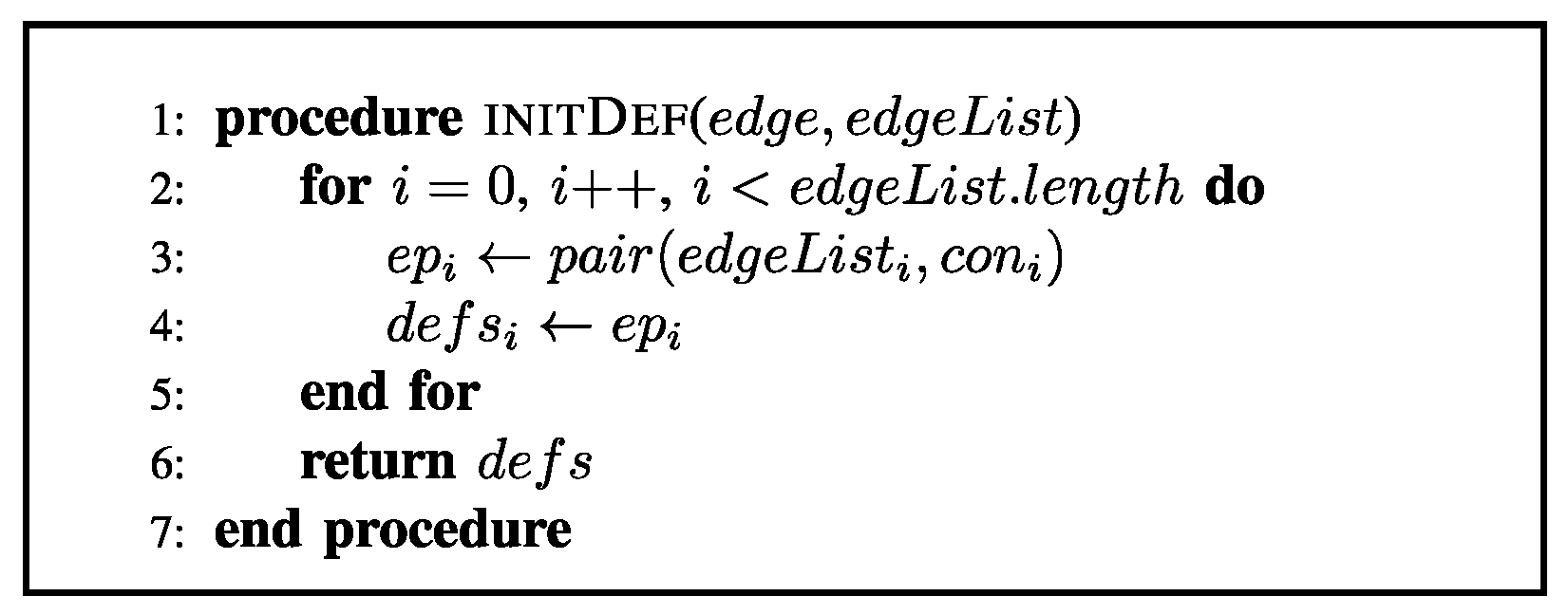
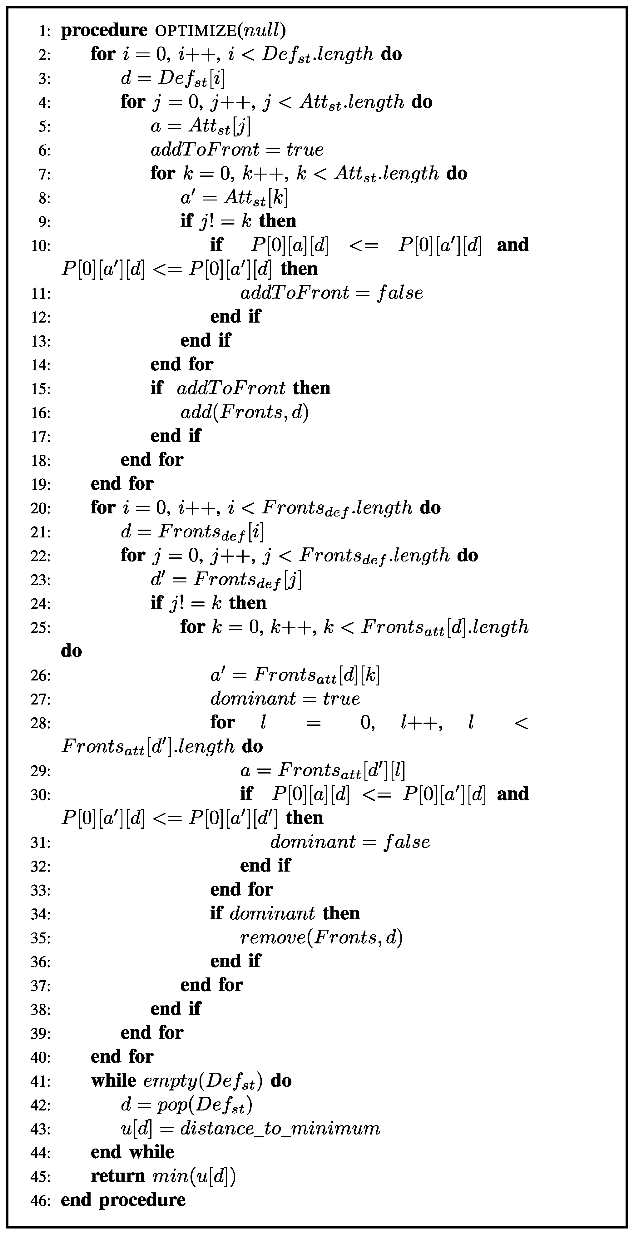
The implementation consists of creating a game, creating defense strategies, creating attack strategies, running the game by going over all possible attack and defense strategy pairings, and finally using Pareto Optimization to determine the optimal strategy. The pseudo codes are listed below.

In Figure 1, Figure 2, Figure 3 and Figure 4, the implementation and simulation of the model was custom coded in our Pareto Defense Strategy Selection Simulator PDSSS. This custom simulator was written in Python, with the numpy library. It comfortably runs on a MacBook Pro 2016 model machine (MacOS Sierra Version 10.12.6) with an Intel Core i5 (dual-core 3.1 GHz) CPU and 8 GB RAM.

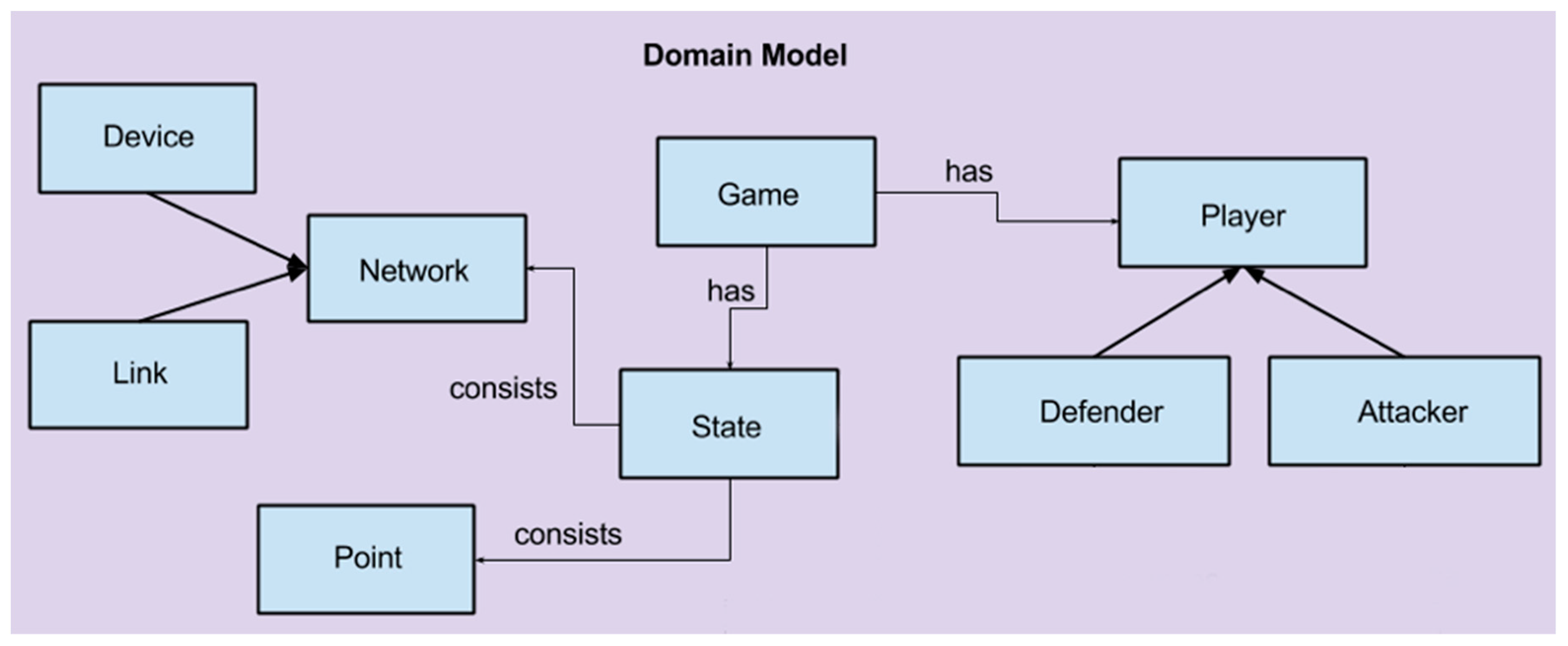
This version of the model is primarily concerned with calculating and presenting the Pareto Optimal attack and defense strategy. The implementation consists of the creation of graph objects and a controlling game object that the actual calculation, as per the above pseudocode. Figure 5 shows the domain model for this section of the PDSSS. For visualization purposes, we used the standard python visualization package, Tkinter.

4. Experiment Results Analysis

Using the algorithm described in the implementation, we set up an experiment using a network simulation with two servers and four client vertices. The experiment shows how the algorithm can be used to choose an effective strategy for a defender facing a set of possible attack strategies. The experiment functions as a proof of concept for the approach detailed in the previous sections.

4.1. Graph Instance

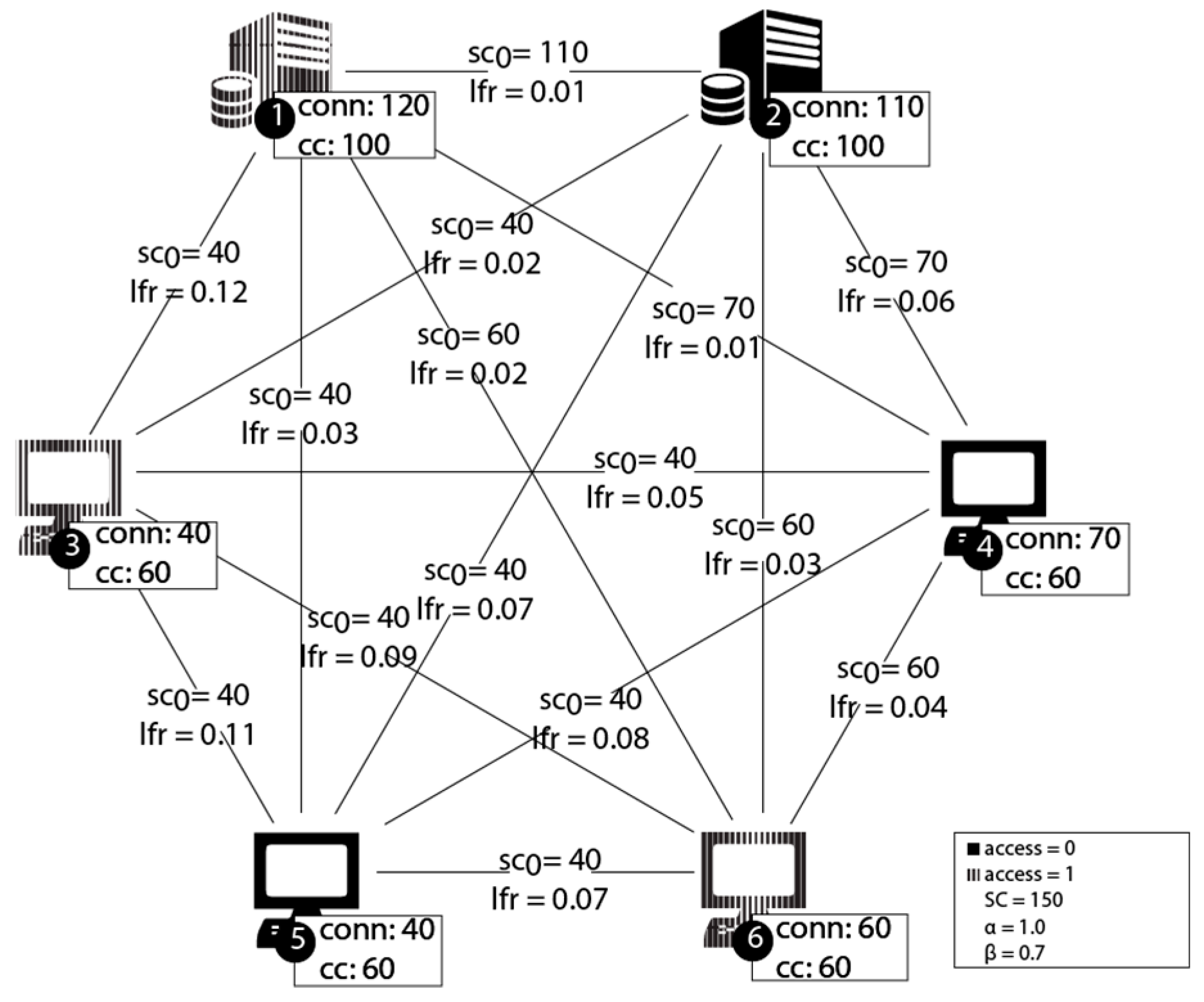
As described in the graph definition, the devices are connected as a full graph. The servers are distinguished from the client, by having more connections, more stable connections and being more expensive to capture. Three of the devices are susceptible to capture and thus can function as a starting point for an attack chain. The initial network setup is shown in Figure 6.

4.2. Strategies Instance

The game consists of one defender and one attacker. The defender strategies consist of adjusting the number of shared connections between the vertices. He can do this by adjusting the number of available connection on a given vertex.

As described in the defender strategy, the defender actually adjusts the number of available ports in a vertex. The result is that all the edges connected to that vertex now have a lower maximum for their shared connections. Because Formulas (21) and (24) use the shared connections on the link, it seems more prudent to describe the defense strategy in terms of shared connections on the link, rather than the explicit change in open vertex ports.

The defender in this game has fivestrategies available. See

Table 1. Defense Strategies.

	Description	Strategy
Sdefense(1)	High connections everywhere	+10, +80, +50, …, +80, +60, +80
Sdefense(2)	Low connections everywhere	−80, −10, −40, …, −10, −30, −10
Sdefense(3)	Med connections everywhere	−50, +20, −10, …, +20, 0, +20
Sdefense(4)	High server, Med clients	+40, +30, 0, …, +30, +10, +30
Sdefense(5)	No connections to vulnerable devices	−110, −40, −70, …, 0, −60, −40

for a short description of the strategies and Figure 7 for an example of a single strategy. Strategy (1) is an attempt to just maximize connectivity and bearing the cost of an attack. This would be the equivalent of a do-nothing approach and suitable for a situation where the cost of a defense exceeds the benefit gained. Strategy (2) describes an attempt to decrease the connectivity, closing as many ports as possible. This decreases network efficiency, but makes it less likely for an attack to be successful. Strategy (3) is a balance between Strategies (1) and (2). The idea here is that a medium defense will stop the most egregious attacks, but not do much against smaller attacks. Strategy (4) tries to flow as much traffic through the servers as possible. The higher protection costs makes attacks on the servers more expensive and the lower lfr of the server links makes sure that there is always traffic flowing through the best links. Strategy (5) is an attempt to quarantine the vulnerable vertices.

Figure 7 shows Defense Strategy 5, which consists of decreasing the shared connections with vulnerable vertices to zero. Figure 7 shows the change in each corresponding edge. This would decrease, for example, the number of shared connections on link (3,4) from 40 to 40 − 40 = 0.

The attacker’s strategy is a two-step process that requires the attacker to first capture a vertex and then launch attack chains from the captured vertex. The attacker has five strategies available. See

Table 2. Attack strategies.

	Description	Strategy
Sattack(1)	Strong server attack, strong client attack	110:(1,2), 40:(3,5,6), 60:(1,6,2)
Sattack(2)	Strong client attack, long attackchain	40:(3,4,5,6,1,2), 60:(6,4,1)
Sattack(3)	Strong server attack, long attackchain	30:(3,4,5,6,1,2), 120:(1,2)
Sattack(4)	Weak server attack, weak client attack	80:(1,2,4), 40:(6,5,1)
Sattack(5)	All attacks from one device	50:(1,6,2,3), 50:(1,4,6,5)

for a short description of the strategies.

Strategy (1) is an attempt to bring down as many shared connections as possible in as many places as possible. It contains the most attack chains of the strategies and tries to bring down the largest number of shared connections. Strategy (2) ignores the expensive servers and targets the cheaper client machines. This should yield a better cost–benefit for the attacker. Strategy (3) tries to take down the server connection and uses a single long attack chain to strike every vertex in the network. Strategy (4) tries a weak attack on a variety of vertices. The idea is that a well-protected system will not allow for many shared connections, so it may be better to make small distributed attacks. Attack (5) tries to safe cost by capturing just one node and orchestrating all attacks from there.

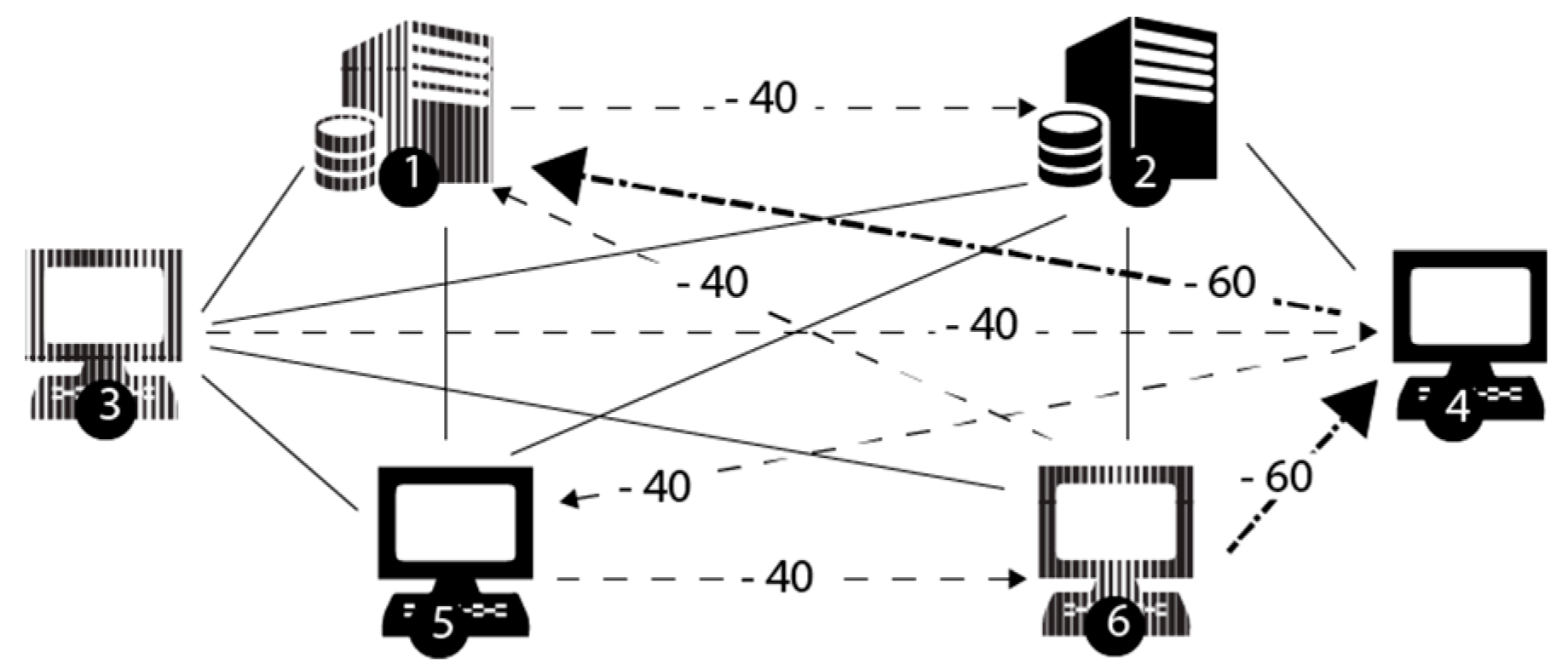
See Figure 8 for an example of a single strategy. The figure shows Attack Strategy 2, which consists of two attack chains. The first attack chain starts at vertex 3 and creates a chain that touches all the vertices in the network, using the following path 3→4→5→6→1→2. The attacker attempts to decrease the shared connections for each link it traverses by 40.

Note that the actual number of shared connections effected cannot be less than the number minimum number of connections allowed in each step of the chain. If the defender had implemented Strategy 3 (see Figure 8), the number of shared connections on link (3,4) would be 0. Hence, at no point in the chain could the attacker decrease the shared connections to by more than 0. The second chain is 6→4→1. Here, the attacker tries to decrease the shared connections by 60 at each step. Once again, a defense strategy may bottleneck the attack chain.

4.3. Pareto Optimization Process

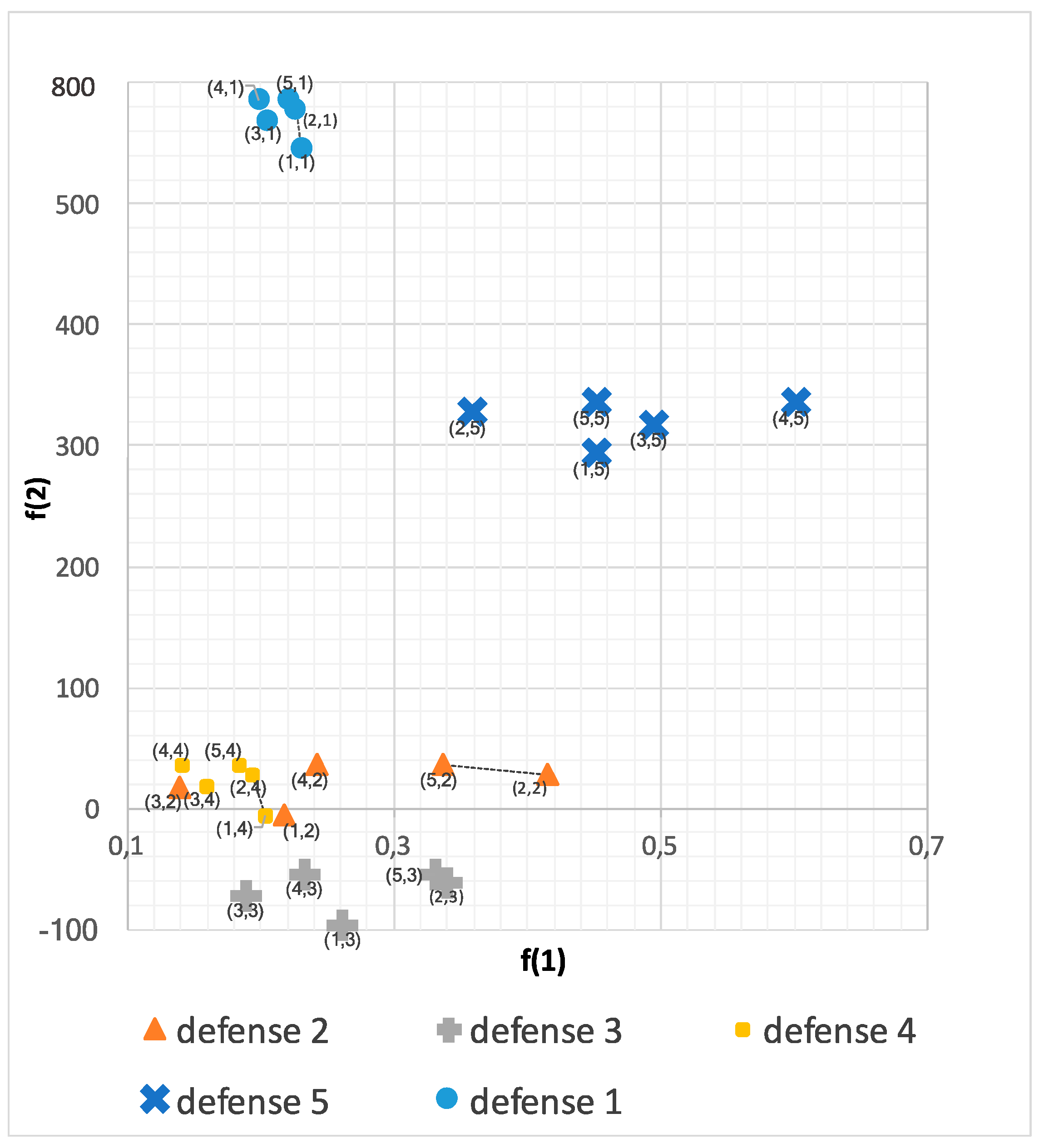
Once we have determined the strategies, we can calculate the payment functions for all 25 strategy pairings. The results are in

Table 3. Goal function results.

Sattack	Sdefense	fa,d(1)	fa,d(2)	Sattack	Sdefense	fa,d(1)	fa,d(2)
1	1	0.230927	664	4	3	0.232278	−54
2	1	0.22626	698	5	3	0.330647	−54
3	1	0.205723	688	1	4	0.202966	−6
4	1	0.19896	706	2	4	0.194094	28
5	1	0.221122	706	3	4	0.159428	18
1	2	0.217027	−6	4	4	0.140303	36
2	2	0.414527	28	5	4	0.183784	36
3	2	0.138739	18	1	5	0.451892	294
4	2	0.24226	36	2	5	0.358722	328
5	2	0.33678	36	3	5	0.494595	318
1	3	0.261064	−96	4	5	0.601351	336
2	3	0.339981	−62	5	5	0.451892	336
3	3	0.188249	−72

. Figure 9 shows the results in the target space in the defender’s view. Here each defense strategy has the same marker.

To determine the optimal defense strategy, we first must calculate the attacker’s Pareto fronts for each defense strategy.

First, we divide the results by defense strategy. This gives us the five groups visible in Figure 9. Circles represent Defense (1), triangles Defense (2), plusses Defense (3), squares Defense (4), and crosses Defense (5).

Next, we calculate the attacker’s Pareto front for each defense strategy. Remember that the attacker wishes to maximize the outcomes. Therefore, we must use Formula (31). As an example, we can look at Defense (2) which has the following points (0.217, −6), (0.415, 28), (0.139, 18), (0.242, 36), (0.337, 36).

The Pareto front only contains points that are not dominated by another point in the set. A point by point analysis of Defense (2) gives us:

-

(0.217, −6) is dominated by (0.415, 28), (0.242, 36) and (0.337, 36) => not in the Pareto front.

-

(0.415, 28) is not dominated by any point => is in the Pareto front.

-

(0.139, 18) is dominated by (0.415, 28), (0.242, 36) and (0.337, 36) => not in the Pareto front.

-

(0.242, 36) is dominated by (0.337, 36) => not in the Pareto front.

-

(0.337, 36) is not dominated by any point => is in the Pareto front.

The result is that the Pareto front for Defense (2) is {(2,2), (5,2)}. Note that the number here refer to attack strategy and defense strategy, f_2,2 and f_5,2.

Going through all the defenses in a similar manner, we get the following fronts: {(1,1), (2,1), (4,1)}, {(2,2),(5,2)}, {(2,3),(5,3)}, {(1,4),(2,4),(5,4)}, {(4,5)}

Next, we remove all dominated fronts. This is done using Formula (29). Using the front of Defense Strategy (2) as an example, we can once again do a point by point analysis. Note that this time we are trying to minimize, hence we are looking for a point where the values are lower.

-

(0.415, 28) is dominated by (0, 203, −6).

-

(0.337, 36) is dominated by (0, 203, −6).

As we can see, there exists a point that dominates all the points in Strategy (2). The point (0, 203, −6) is the output of f_1,4. This means Defense Strategy (2) is dominated by Defense Strategy (4). We thus remove Defense Strategy (2) from the set of non-dominated defense strategies.

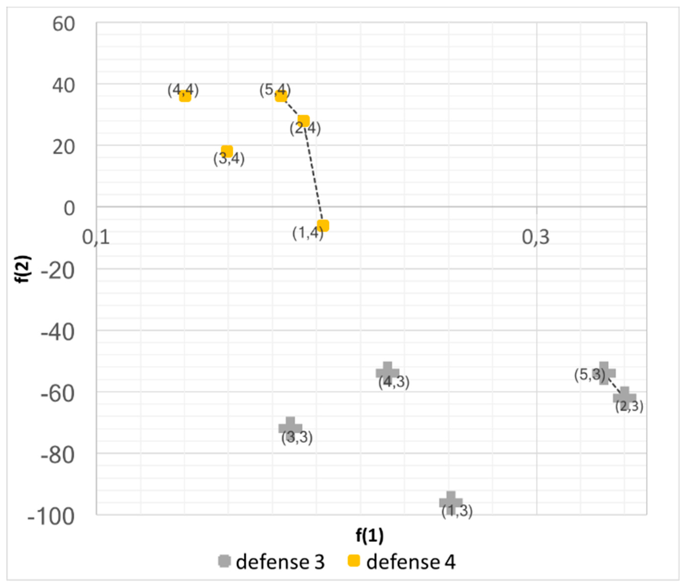
If we apply the same step by step set domination calculation for all the fronts, we are left with: {(2,3),(5,3)}, {(1,4),(2,4),(5,4)}. These are the non-dominated defense strategies and are visible in Figure 10.

Finally, we rank the strategies using Formula (38). This gives us $u(s_{defense}^3)$ = 0.972 and $u(s_{defense}^4)$ = 0.835. Thus, the best defense strategy is Defense Strategy 4.

4.4. Comparison to Nash Equilibrium

We compare the results of the Pareto Optimization problem with a simple minimax approach. The minimax solution for zero-sum game is the same as the Nash Equilibrium for the game. The Nash Equilibrium is a state in which no player can gain by changing only his own strategy, assuming that his opponent does not change their strategy. Generally, the Nash Equilibrium solution is the best solution possible for a player. As such, a comparison with the minimax algorithm should give us a measure of how well our approach performs.

Because minimax requires single value, we first need to scalarize the results of the goal function. We can do this by taking the normalized distance to the absolute minimum, as described in Formula (39). Note that this is a simplification of Formula (38).

$$u({\overline{f}}_{a,d})=\sqrt{{\displaystyle \sum }_{k=1}^K{\left(\frac{f_{a,d}^{(k)}-f_{min}^{(k)}}{f_{max}^{(k)}-f_{min}^{(k)}}\right)}^2}$$

(39)

The scalarized results for the attack and defense interactions is given in

Table 4. Scalarized results for attack and defense interactions.

Sattack	Sdefense	u(fa,d)	Sattack	Sdefense	u(fa,d)
1	1	0.968	4	3	0.209
2	1	1.008	5	3	0.418
3	1	0.988	1	4	0.179
4	1	1.008	2	4	0.196
5	1	1.016	3	4	0.149
1	2	0.203	4	4	0.165
2	2	0.616	5	4	0.264
3	2	0.142	1	5	0.191
4	2	0.278	2	5	0.833
5	2	0.459	3	5	0.711
1	3	0.264	4	5	0.926
2	3	0.437	5	5	1.136
3	3	0.111

. Taking the minimum of the max of every defense strategy gives Strategy (5,4). That means the minimax algorithm confirms that the best defense strategy is Strategy 4.

The experiment discussed in the previous section is only one of a possible set of attack and defense configurations. To test the algorithm, we ran the Pareto Optimization function and the Minimax function for 1000 randomly generated networks. The networks were randomly generated using the configuration given in

Table 5. Possible Network configurations.

Network Configurations
Number of nodes	20–50
Number of attack options	12
Number of defense options	12
Node capture costs	50–100
Link fail rate	0.00–0.15
Alpha	0.75–1.00
Beta	0.35–0.60

. Where possible, configuration values were randomly selected from the specified ranges.

The results of the repeated experiment confirm those found in the detailed experiment. The efficiency of the Pareto Optimization approach is comparable to the Minimax algorithm (only 1% slower). For 38% of the networks, the Pareto Optimal solution was also the Nash Equilibrium. The results are in

Table 6. Results of Experiment for different configurations.

Network Results
Number of configurations	1000
Average duration Pareto	1.93 ms
Average duration Minimax	1.91 ms
Average difference between Pareto solutions and Nash Equilibrium	0.0027
Pareto solutions includes Nash Equilibrium	38.3%

.

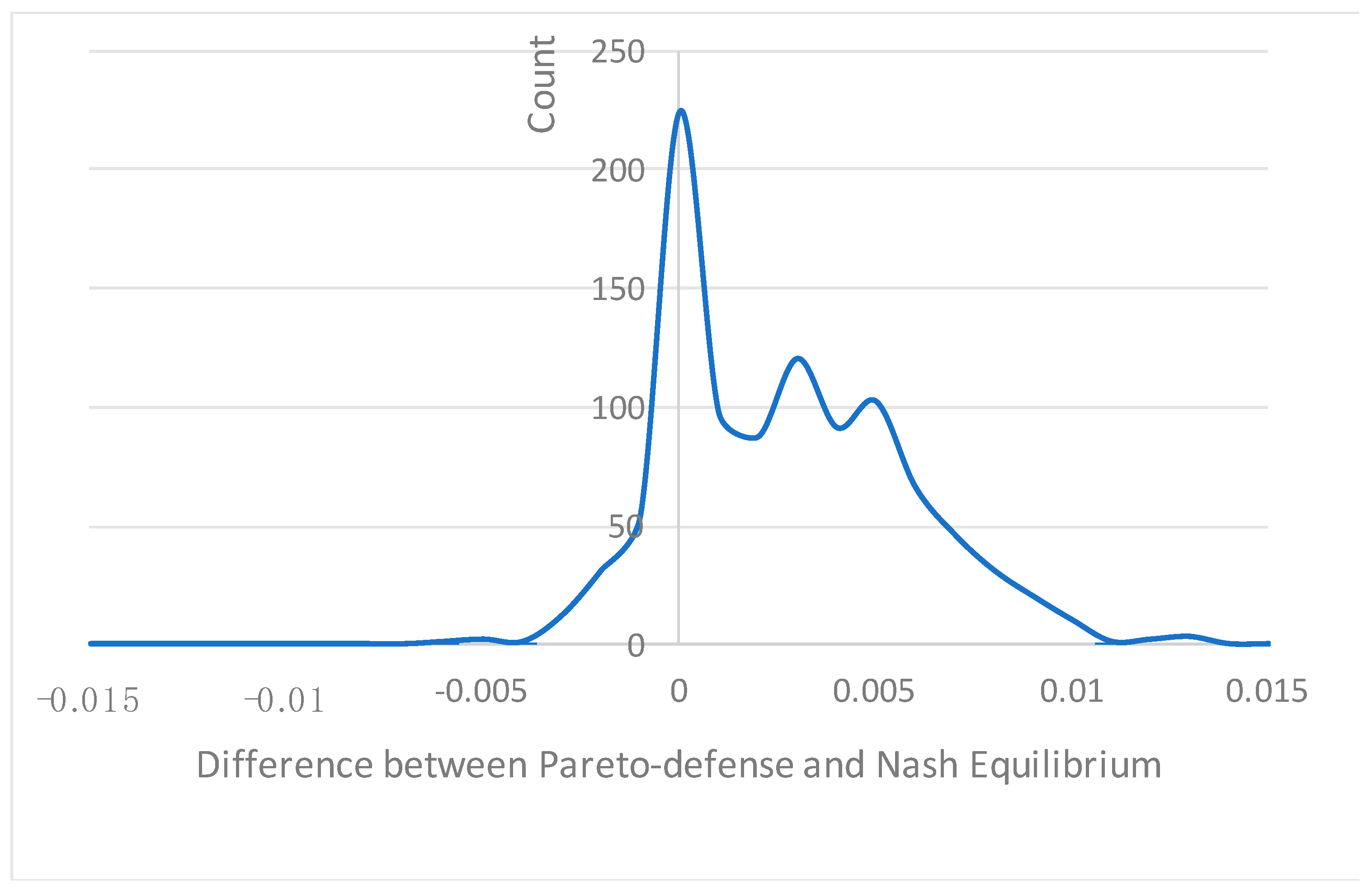
The Pareto Optimal solution set does not always include the Nash Equilibrium solution. It is informative to compare the two by an objective measure. As objective measure, we use the difference in average distance to the minimum for a defense strategy. The average distance to the minimum ($DTM$) for a defense strategy is calculated using Formula (38). The formula takes the normalized values for each goal dimension and scalarizes it with equal weights. The goal of the defender is to minimize the network results, thus the smaller the average distance, the better the algorithm.

We compare the minimax approach with the Pareto approach, by subtracting the $DTM$ of the minimax from that of the Pareto solution. See Formula (40).

$$DT{M}_{difference}= DT{M}_{pareto}-DT{M}_{minimax}$$

(40)

The results show that the defense chosen by the Pareto Optimal solution tend to be slightly inferior to the Nash Equilibrium. In other words, the Pareto approach chooses. The difference is visible in Table 6 and Figure 11.

Despite seeming inferior, the Pareto approach does offer large advantages over a minimax calculation. The minimax algorithm, like all Nash Equilibrium calculations require that you know the goal preferences before calculation of the equilibrium point. The Pareto approach, however, does not require prior knowledge of the goal preferences.

Another advantage is that of subjective choice. The minimax algorithm produces a single Nash Equilibrium point. By contrast, the Pareto Optimization approach results in a shortlist of non-dominated strategies. This gives the final choice to security managers, who can use a variety of subjective selection methods to determine which strategy he feels is best.

In our experiment, the Pareto Optimization approach resulted in the set of possible defense choices being brought down from 12 to an average of 2. The advantage of this should be clear to security managers who want to whittle their options down to a manageable number. The decrease in options is visible in Figure 12.

5. Discussion

This paper shows how to optimize strategy for network using a Pareto Optimization in a zero-sum information incomplete game. The main contribution is the quantifying relevant network characteristics and player goals and applying Pareto Optimization to these. The quantification provides approach that network defenders can use to determine an optimal strategy.

This includes two noticeable improvements on existing research using Pareto Optimization for security strategy. The first being that we have allowed for the implementation of strategy on a device level, which is a more realistic representation of how defense strategy is actually implemented. Previous studies such as Eisenstadt [35] focused on the link level availability, which ignores the effect on the vertices. The link level focus means that it ignores the wider effect that a single vertex failure may have in network. The value of capturing a server, rather than a client machine lies in the fact that the servers function as nexus points to which the vast majority of nodes will connect. Capturing a single server can be a far more effective strategy than capturing a set of clients, due to the network effect of the server.

Despite this difference, our results are consistent with those of Eisentstadt, who also showed that Pareto Optimization allows for the estimation of an effective defense strategy. In addition, our research shows that the optimization, while useful, does not yield solutions that are superior to a Nash Equilibrium.

The second is that in Formula (38) we have an objective approach to choosing an ideal strategy from the remaining non-dominated Pareto fronts.

The included experiment an implementation shows that that the approach works in practice and allowed us to find an optimal defense for a simulated network.

The experiment was carried out with a specific implementation for the payment function, but the theory indicates that the same model can be used with a variety of payment functions and an arbitrary number of dimensions. In fact, any arbitrary deterministic function can be applied, including chaos functions.

This experiment singles out the effect of the Pareto Optimization on strategy selection. Different models can include features that aid the selection of a defense strategy. The authors of this paper have studied the selection of a defense strategy using a combination of Pareto Optimization and reinforcement learning [18]. However, that model requires frequent interaction between the attacker and defender. The simulation for the previously studied dynamic model assumes that the defender has enough information about the attacker to not only model his behavior, but that the behavior remains the same throughout the interactions.

A more static model, such as the one presented here, can be used to: (1) disentangle the effect of Pareto Optimization from the learning algorithm; and (2) the creation of a system that can easily look at different attack strategies. As indicated above, we can use this same game model, with different payment functions or goals/dimensions. The effectiveness of a defense strategy can thus be quickly tested with a simple modification to this static model.

6. Conclusions

The approach described provides a fresh perspective on other network policy optimization problems, most of which tend to view a defense strategy that leads to a Nash Equilibrium state as optimal. Our experiment shows that the approach does not always result in a nash equilibrium state. However, we feel confident that the advantage of choice, outweighs this.

The pareto optimization approach allows for multiple interactions between the attacker and defender. This allows for a more realistic approach to network defense, as the both the attacker and defender of a network can change their strategies after a single interaction. We have expanded the concept described here and create a dynamic model that details multiple interactions between attacker and defender [25].

Finally, we would like to point out that the model is not dependent on a specific payment function.

References

- Stolfo, S.J.; Fan, W.; Lee, W.; Prodromidis, A.; Chan, P.K. Cost-based modeling for fraud and intrusion detection: Results from the JAM project. In Proceedings of the DARPA Information Survivability Conference and Exposition, DISCEX’00, Hilton Head, SC, USA, 25–27 January 2000; Volume 2. [Google Scholar]
- Bistarelli, S.; Fioravanti, F.; Peretti, P. Defense trees for economic evaluation of security investments. In Proceedings of the First International Conference on Availability, Reliability and Security, Vienna, Austria, 20–22 April 2006. [Google Scholar]
- Gordon, L.A.; Loeb, M.P. Budgeting process for information security expenditures. Commun. ACM 2006, 49, 121–125. [Google Scholar] [CrossRef]
- Viduto, V.; Huang, W.; Maple, C. Toward optimal multi-objective models of network security: Survey. In Proceedings of the 17th International Conference on Automation and Computing (ICAC), Huddersfield, UK, 10 September 2011. [Google Scholar]
- Feng, N.; Wang, H.J.; Li, M. A security risk analysis model for information systems: Causal relationships of risk factors and vulnerability propagation analysis. Inf. Sci. 2014, 256, 57–73. [Google Scholar] [CrossRef]
- Roy, S.; Ellis, C.; Shiva, S.; Dasgupta, D.; Shandilya, V.; Wu, Q. A survey of game theory as applied to network security. In Proceedings of the 43rd Hawaii International Conference on System Sciences (HICSS), Honolulu, HI, USA, 5–8 January 2010. [Google Scholar]
- Carin, L.; Cybenko, G.; Hughes, J. Cybersecurity strategies: The queries methodology. Computer 2008, 41. [Google Scholar] [CrossRef]
- Lye, K.W.; Wing, J. Game strategies in network security. Int. J. Inf. Secur. 2005, 4, 71–86. [Google Scholar] [CrossRef]
- Shapley, L.; Rigby, F.D. Equilibrium points in games with vector payoffs. Nav. Res. Logist. 1959, 6, 57–61. [Google Scholar] [CrossRef]
- Osborne, M.J.; Ariel, R. A Course in Game Theory; Massachusetts Institute of Technology (MIT): Cambridge, MA, USA, 1994. [Google Scholar]
- Dainotti, A.; Pescapé, A.; Ventre, G. Worm traffic analysis and characterization. In Proceedings of the IEEE International Conference on Communications, ICC’07, Glasgow, UK, 24–28 June 2007; pp. 1435–1442.
- Boyle, P. Idfaq: Distributed Denial of Service Attack Tools: Trinoo and Wintrinoo. 2000. Available online: https://www.sans.org/security-resources/idfaq/distributed-denial-of-service-attack-tools-trinooand-wintrinoo/9/10 (accessed on 1 November 2016).
- Specht, S.M.; Lee, R.B. Distributed denial of service: Taxonomies of attacks, tools, and countermeasures. In Proceedings of the ISCA 17th International Conference on Parallel and Distributed Computing Systems, The Canterbury Hotel, San Francisco, CA, USA, 15–17 September 2004; pp. 543–550. [Google Scholar]
- Hallman, R.; Bryan, J.; Palavicini, G.; Divita, J.; Romero-Mariona, J. IoDDoS—The Internet of Distributed Denial of Sevice Attacks—A Case Study of the Mirai Malware and IoT-Based Botnets. In Proceedings of the 2nd International Conference on Internet of Things, Big Data and Security (IoTBDS 2017), Porto, Portugal, 24–26 April 2017; pp. 47–58. [Google Scholar]
- Woolf, N. Ddos Attack that Disrupted Internet Was Largest of Its Kind in History, Experts Say. 2016. Available online: https://www.theguardian.com/technology/2016/oct/26/ddos-attack-dyn-mirai-botnet (accessed on 22 October 2016).
- Santanna, J.J.; Durban, R.; Sperotto, A.; Pras, A. Inside Booters: An Analysis on Operational Databases. In Proceedings of the 14th IFIP/IEEE International Symposium on Integrated Network Management (IM), Ottawa, ON, Canada, 11–15 May 2015. [Google Scholar]
- Pras, A.; Santanna, J.J.; Steinberger, J.; Sperotto, A. DDoS 3.0-How terrorists bring down the internet. In Proceedings of the International GI/ITG Conference on Measurement, Modelling, and Evaluation of Computing Systems and Dependability and Fault Tolerance, Munster, Germany, 4 April 2016; Springer: Cham, Germany, 2016; pp. 1–4. [Google Scholar]
- Casenove, M.; Armando, M. Botnet over Tor: The illusion of hiding. In Proceedings of the IEEE 6th International Conference Cyber Conflict (CyCon 2014), Tallinn, Estonia, 3–6 June 2014. [Google Scholar]
- Abu Rajab, M.; Zarfoss, J.; Monrose, F.; Terzis, A. A multifaceted approach to understanding the botnet phenomenon. In Proceedings of the 6th ACM SIGCOMM Conference on Internet Measurement, IMC’06, Rio de Janeriro, Brazil, 25–27 October 2006; pp. 41–52. [Google Scholar]
- Dainotti, A.; King, A.; Claffy, K.; Papale, F.; Pescapé, A. Analysis of a/0 stealth scan from a botnet. In IEEE/ACM Transactions on Networking (TON); IEEE Press: Iscataway, NJ, USA, 2015; Volume 23, pp. 341–354. [Google Scholar]
- Dainotti, A.; Pescapé, A.; Ventre, G. A cascade architecture for DoS attacks detection based on the wavelet transform. J. Comput. Secur. 2009, 17, 945–968. [Google Scholar] [CrossRef]
- Abshoff, S.; Cord-Landwehr, A.; Jung, D.; Skopalik, A. Multilevel Network Games. In Proceedings of the International Conference on Web and Internet Economics, Beijing, China, 14–17 December 2014. [Google Scholar]
- Liang, X.; Xiao, Y. Game theory for network security. IEEE Commun. Surv. Tutor. 2013, 15, 472–486. [Google Scholar] [CrossRef]
- Manshaei, M.H.; Zhu, Q.; Alpcan, T.; Basar, T.; Hubaux, J.-P. Game Theory Meets Network Security and Privacy. ACM Comput. Surv. 2011, 45. [Google Scholar] [CrossRef]
- Sun, Y.; Xiong, W.; Yao, Z.; Moniz, K.; Zahir, A. Network Defense Strategy Selection with Reinforcement Learning and Pareto Optimization. Appl. Sci. 2017, 7, 1138. [Google Scholar] [CrossRef]
- Sun, Y.; Li, Y.; Xiong, W.; Yao, Z.; Moniz, K.; Zahir, A. Pareto Optimal Solutions for Network Defense Strategy Selection Simulator in Multi-Objective Reinforcement Learning. Appl. Sci. 2018, 8, 136. [Google Scholar] [CrossRef]
- Wu, Q.; Shiva, S.; Roy, S.; Ellis, C.; Datla, V. On modeling and simulation of game theory-based defense mechanisms against DoS and DDoS attacks. In Proceedings of the 2010 Spring Simulation Multiconference, Society for Computer Simulation International, Orlando, FL, USA, 11–15 April 2010; p. 159. [Google Scholar]
- Studer, A.; Perrig, A. The Coremelt attack. In Proceedings of the European Symposium on Research in Computer Security, Saint-Malo, France, 21–23 September 2009; Springer: Berlin/Heidelberg, Germany, 2009; pp. 37–52. [Google Scholar]
- Matalon-Eisenstadt, E.; Moshaiov, A.; Avigad, G. The competing travelling salespersons problem under multi-criteria. In Proceedings of the International Conference on Parallel Problem Solving from Nature, Edinburgh, UK, 17–21 September 2016. [Google Scholar]
- Bonaci, T.; Linda, B. Node capture games: A game theoretic approach to modeling and mitigating node capture attacks. In Proceedings of the International Conference on Decision and Game Theory for Security, College Park, MA, USA, 14 November 2011; Springer: Berlin/Heidelberg, Germany; pp. 44–55. [Google Scholar]
- NotPetya Technical Analysis—A Triple Threat: File Encryption, MFT Encryption, Credential Theft. Available online: https://www.crowdstrike.com/blog/petrwrap-ransomware-technical-analysis-triple-threat-file-encryption-mft-encryption-credential-theft/ (accessed on 29 June 2017).
- Zeleny, M. Games with multiple payoffs. Int. J. Game Theory 1975, 4, 179–191. [Google Scholar] [CrossRef]
- Welch, D. Adversary Threat Taxonomy. In Proceedings of the IEEE Information Assurance Workshop, West Point, NY, USA, 17–19 June 2002. [Google Scholar]
- Schneider, B. Attack Trees: Modeling Security Threats. Dr. Dobb’s J. 2000, 1, 5. [Google Scholar]
- Eisenstadt, E.; Moshaiov, A. Novel Solution Approach for Multi-Objective Attack-Defense Cyber Games with Unknown Utilities of the Opponent. IEEE Trans. Emerg. Top. Comput. Intell. 2017, 1, 16–26. [Google Scholar] [CrossRef]
Figure 1.
Pseudocode for Initialize Defense.
Figure 2.
Pseudocode for Initialize Offense.
Figure 3.
Pseudocode for game.
Figure 4.
Pseudocode for Pareto Optimization.
Figure 5.
PDSSS domain model (truncated to only include Pareto Optimization).
Figure 6.
Network at initial state.
Figure 7.
Defense Strategy 5.
Figure 8.
Attack Strategy 2.
Figure 9.
Target space in defender’s view.
Figure 10.
Target space with remaining Pareto fronts.
Figure 11.
Histogram for difference between Pareto-defense and Nash Equilibrium strategies.
Figure 12.
Histogram for number of non-dominated defense strategies.