
DMFF-Net: Densely Macroscopic Feature Fusion Network for Fast Magnetic Resonance Image Reconstruction

School of Electrical and Information Engineering, Tianjin University, Tianjin 300072, China
*
Author to whom correspondence should be addressed.
Electronics 2022, 11(23), 3862; https://doi.org/10.3390/electronics11233862
Submission received: 23 September 2022
/
Revised: 2 November 2022
/
Accepted: 4 November 2022
/
Published: 23 November 2022
(This article belongs to the Collection Deep Learning for Computer Vision: Algorithms, Theory and Application)
Abstract
:The task of fast magnetic resonance (MR) image reconstruction is to reconstruct high-quality MR images from undersampled images. Most of the existing methods are based on U-Net, and these methods mainly adopt several simple connections within the network, which we call microscopic design ideas. However, these considerations cannot make full use of the feature information inside the network, which leads to low reconstruction quality. To solve this problem, we rethought the feature utilization method of the encoder and decoder network from a macroscopic point of view and propose a densely macroscopic feature fusion network for fast magnetic resonance image reconstruction. Our network uses three stages to reconstruct high-quality MR images from undersampled images from coarse to fine. We propose an inter-stage feature compensation structure (IFCS) which makes full use of the feature information of different stages and fuses the features of different encoders and decoders. This structure uses a connection method between sub-networks similar to dense form to fuse encoding and decoding features, which is called densely macroscopic feature fusion. A cross network attention block (CNAB) is also proposed to further improve the reconstruction performance. Experiments show that the quality of undersampled MR images is greatly improved, and the detailed information of MR images is enriched to a large extent. Our reconstruction network is lighter than many previous methods, but it achieves better performance. The performance of our method is about 10% higher than that of the original method, and about 3% higher than that of most existing methods. Compared with the nearest optimal algorithms, the performance of our method is improved by about 0.01–0.45%, and our computational complexity is only 1/14 of these algorithms.
1. Introduction
Magnetic resonance imaging (MRI) is a widely used medical imaging technology in the field of modern medicine [1]. This non-invasive imaging method can provide high-resolution structural, anatomical, and functional information as well as excellent contrast of soft tissue without ionizing radiation [2]. Thus, it has become a necessity in the fields of psychiatry, medicine, radiology, and so on.
K-space undersampling is usually a common method to speed up MRI scanning. This method can achieve the purpose of speeding up by reducing the number of k-space traversals during acquisition, but this method does not meet the Nyquist sampling theorem and will generate aliasing artifacts during reconstruction [1]. Therefore, people have explored traditional reconstruction methods such as compressed sensing [3] and parallel imaging [4]. The compressed sensing algorithm uses a nonlinear process to reconstruct images from undersampled k-space data. Parallel imaging is accelerated by multi-channel k-space data. GRAPPA is an algorithm based on k-space reconstruction, which is based on the premise that the collected k-space lines can be used to obtain the lost k-space lines through weighted interpolation [5]. SENSE is an algorithm based on image space correction, which estimates images from k-space by applying prior knowledge to image attributes [6]. These traditional algorithms speed up the scanning of MRI to a certain extent, but these methods adopt iterative calculation, which leads to a long reconstruction time.
With the development of depth learning, more and more people have begun to use depth learning methods to reconstruct MR images [7], segment, classify and detect single-photon emission computed tomography (SPECT) images or positron emission tomography (PET) [8,9,10,11,12]. In the past, deep learning has been widely used in PET and SPECT, including instrumentation and image acquisition/formation, image reconstruction and low-dose/fast image acquisition, quantitative imaging, image interpretation and decision support, and so on [12]. Among these methods, convolutional neural networks (CNNs) are widely used. Some researchers have tried to present a specific CNN architectural component to derive explicit fusion maps [11]. Some researchers have used CNN to classify PET images [10]. The U-Net architecture has also been used for lung cancer lesion segmentation and to fuse the features of the modalities of both PET and CT [9].
Currently, most methods of convolutional neural networks (CNNs) used in MRI reconstruction are based on the encoding and decoding structure of U-Net [13,14,15,16,17]. These methods extract and refine the features of the input image by coding layer by layer, and then restoring the features of the image by decoder, thus achieving a good reconstruction effect. It is worth noting that the skip connection structure in the U-Net network significantly improves the performance of the network. This skip connection links the features of the encoder to the decoder, so that the network can retrieve the lost spatial information in the down sampling of the image and make up the semantic gap of the encoder and decoder [15]. It can be seen that within the network, using the features of the encoder to compensate for the features of the decoder is helpful in improving the reconstruction ability of the network. However, the existing reconstruction algorithms usually adopt simple connection methods such as cascading or parallel connections between networks, which easily leads to semantic gaps between networks and makes insufficient use of the feature information in each sub-network. We call these methods microscopic design ideas.
From a macro point of view, we compared the multistage network to the above-mentioned encoding and decoding network structures. Corresponding to the skip connection within the U-Net, we adopted the skip connection method between networks, making full use of the feature information of the previous network. Through a dense-like connection between sub-networks, the features of encoding and decoding are fully fused, and the encoding ability and decoding ability are enhanced. Our contributions are as follows:
- (1)
- We designed a new encoding and decoding network, and reconstructed high-quality MR images from undersampled images from coarse to fine by adopting three-stage processing.
- (2)
- We propose an inter-stage feature compensation structure (IFCS), which improves the utilization efficiency of features and enhances the encoding and decoding ability by compensating for different encoder and decoder features in different stages. The structure has achieved a significant breakthrough in terms of performance.
- (3)
- Inspired by the self-attention mechanism, we designed a cross network attention block (CNAB), which creatively fuses cross-network features to obtain a global receptive field and further improves the image reconstruction quality.
- (4)
- The experiment shows that our network achieves good performance, which is superior to many previous reconstruction methods and achieves a competitive result in the FastMRI Public Leader board published by Facebook [18].
2. Related Works
We will introduce the related works from three aspects: first, several methods in the field of MR image reconstruction, then the research on the attention mechanism, and finally the related works based on the encoder and decoder structure of U-Net.
2.1. Some Methods in the Field of MR Image Reconstruction
The traditional compressed sensing method [3] realizes the process of image reconstruction from undersampled MR images; Xie et al. [19] summarized the compressed sensing methods and combined deep learning methods with traditional methods; the TV model [20] uses the total-variation penalty, which improves the reconstruction performance; Eo et al. [21] adopted a cross-domain convolutional neural network and introduced a DC layer, and finally proposed KIKI-Net; Ran et al. [22] put forward MD-Recon-Net, which is a network that can process k-space and image space data at the same time, and has achieved good results in removing MR image artifacts; The XPD-Net proposed by Ramzi et al. [23] uses the optimization algorithm to correct the cross-domain network; i- RIM network [24] uses data-driven methods to train the network, which greatly improves the image reconstruction quality and achieves very good performance.
2.2. Attention Mechanism
To better capture long-distance dependencies, Wang et al. [25] proposed the non-local network. Based on the self-attention mechanism [26], they designed a method that can effectively capture global context information. Although the non-local method has achieved good performance, it is not an efficient method because of its huge amount of computation. After that, Hu et al. proposed a very efficient SE-block [27]. This structure caused extensive discussion in academic circles. Over the next few years, SE-block was widely used, and designs based on this structure have emerged in an endless stream. SE-block obtains the importance of each channel through squeezing and exciting operations. Then, according to this importance, the useful features are enhanced and the less useful features suppressed. The global information of the network is used to selectively enhance the useful feature channels and suppress the useless feature channels, to realize the adaptive calibration of feature channels. Compared with non-local, SE-block has fewer parameters, is very convenient to use, and has higher feature processing efficiency. However, compared with the non-local structure, SE-block does not deal with features adequately. To solve this problem, Cao et al. [28] combined these two structures and proposed GC-Net. This structure combines the characteristics of SE-block and non-local and makes a meaningful innovation.
2.3. Encoder and Decoder Network Structure Based on U-Net
The U-Net network [14] was first proposed for cell image segmentation in biology, and its encoding and decoding network can effectively extract image features and refine them step by step. Following that, many scholars put forward increasing numbers of encoding and decoding network structures based on this network for different image processing tasks. Cho et al. [13] proposed a self-spatial, adaptive, and weighted U-Net image segmentation algorithm, which improved the performance of existing methods. In the field of MRI, many reconstruction networks based on U-Net structure have also been born. Ibtehaz et al. [15] deeply analyzed the architecture of the U-Net model and speculated several possibilities of enhancing network performance. According to their analysis, the subtlety of the U-Net is that it connects the corresponding layer of encoder and decoder. However, many disadvantages also exist: the encoder is usually considered low-level semantic information, and the decoder is usually considered high-level semantic information. There may be a semantic gap after connecting the two directly, so the author made some changes to the U-Net network and proposed the idea of MultiRes-Unet; Jha et al. [16] proposed the ResUNet++ network structure, which consists of residual block, SE-block, Atrous pyramid (ASPP), and attention block. The network structure improves the segmentation effect; Zhou et al. [17] also made an analysis on U-Net and put forward U-Net++. They believe that the success of encoding and decoding networks is largely due to their skip connections. This kind of skip connection will combine the shallow, low-level, and fine-grained feature map mapping from the encoding sub-network with the deep, high-level, and coarse-grained feature map mapping from the decoding sub-network. U-Net++ does not tend to choose the network depth. It embeds U-Net with different depths in the architecture. All these U-Nets share one encoder, and their decoders are intertwined. At the skip connection, the aggregation layer is allowed to decide the fusion of different proportions of feature maps and decoder feature maps, instead of just fusing the same scale information.
At present, most encoding and decoding networks only modify the internal structure of the network. Although some methods cascade networks, they only make some simple connections, which do not make full use of the inter-level feature information. To solve this problem, we lighten each network and cascade the networks in a special way to fully share and utilize the feature information. On rethinking the structure of U-Net, we find that the introduction of encoder features greatly improves the decoding ability of the decoder and enriches the semantic information in the decoding stage. With this method, the decoder can fully obtain the spatial information lost due to downsampling in the encoding stage. This idea of feature compensation is very effective. We believe that this method can be expanded. We define this feature compensation method within the network as a microscopic design idea, while we call the feature compensation method between networks a macroscopic design idea. From a macro point of view, we extend the idea of feature compensation from inside the network to between networks, that is, we apply the feature compensation method of U-Net between each sub-network to enhance the decoding ability of the decoder. This idea enables us to obtain very good experimental performance. In addition, inspired by this idea, we also mix the features of the encoder and decoder of the previous network to compensate for the features of the current network encoder. This greatly enhances the coding capability of the network and enriches the semantic information in the coding stage. On this basis, we also designed a cross-network feature attention mechanism to further improve the performance.
Our idea of feature compensation is not limited to the internal structure of the network. It has expanded from microscopic internal network features to macroscopic inter-stage features, and from feature compensation only for decoders to feature compensation for the whole encoding and decoding network. The network parameters are very small, and the whole network is lightweight, but its performance has reached a satisfactory level.
3. DMFF-Net
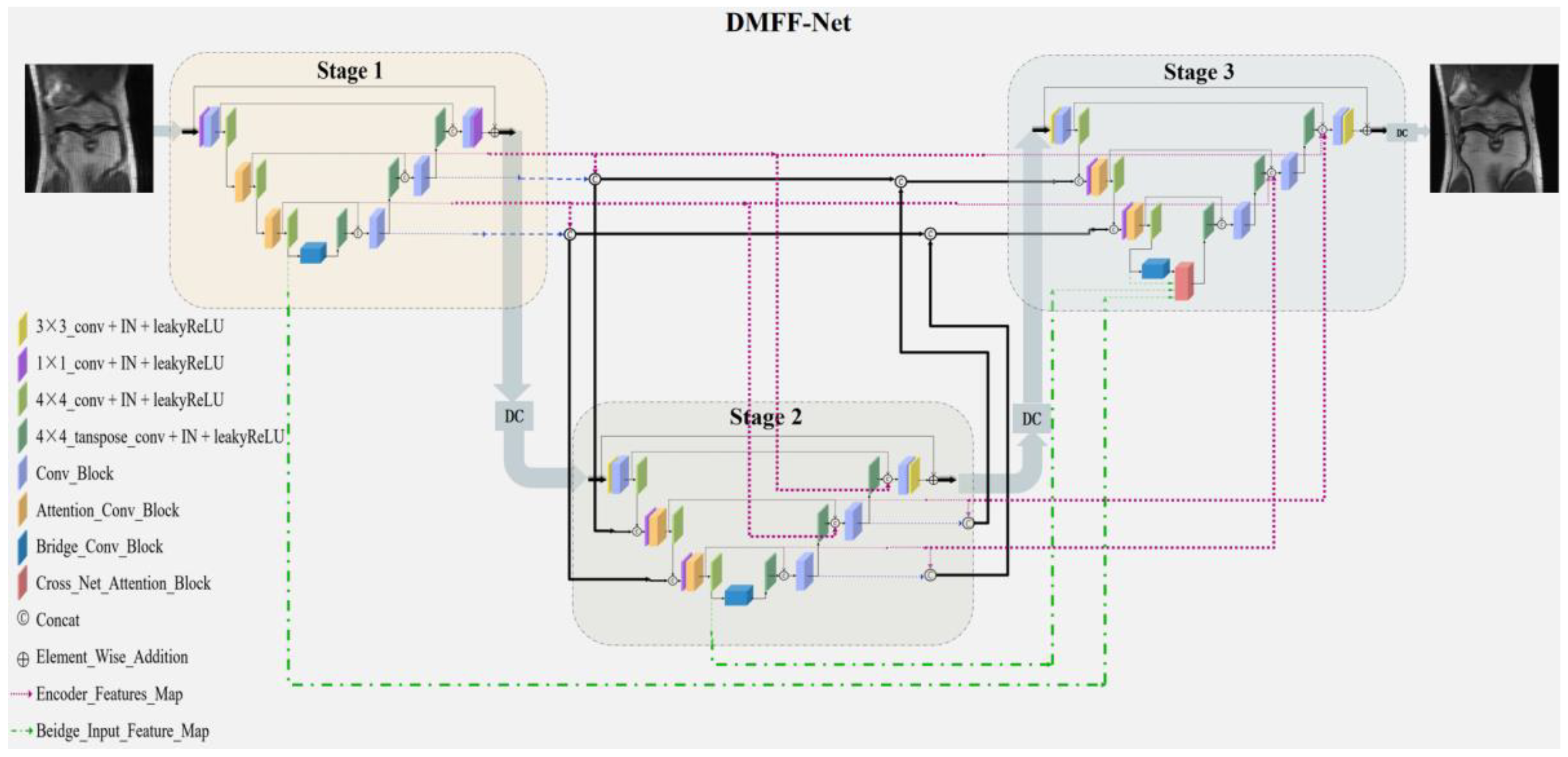
The overall network structure of DMFF-Net is shown in Figure 1. The network consists of three sub-networks. What is considered is not only the internal structure of each sub-network at the micro level, but also the macroscopic feature compensation between networks. The general structure of each sub-network is similar, but the specific details are different. This macro connection design can make full use of the inter-stage features of the network and its connection mode is similar to the macro dense connection between sub-networks. It greatly improves the efficiency of network reconstruction and reduces the difficulty of training.
3.1. Three-Stage Sub-Network Reconstruction
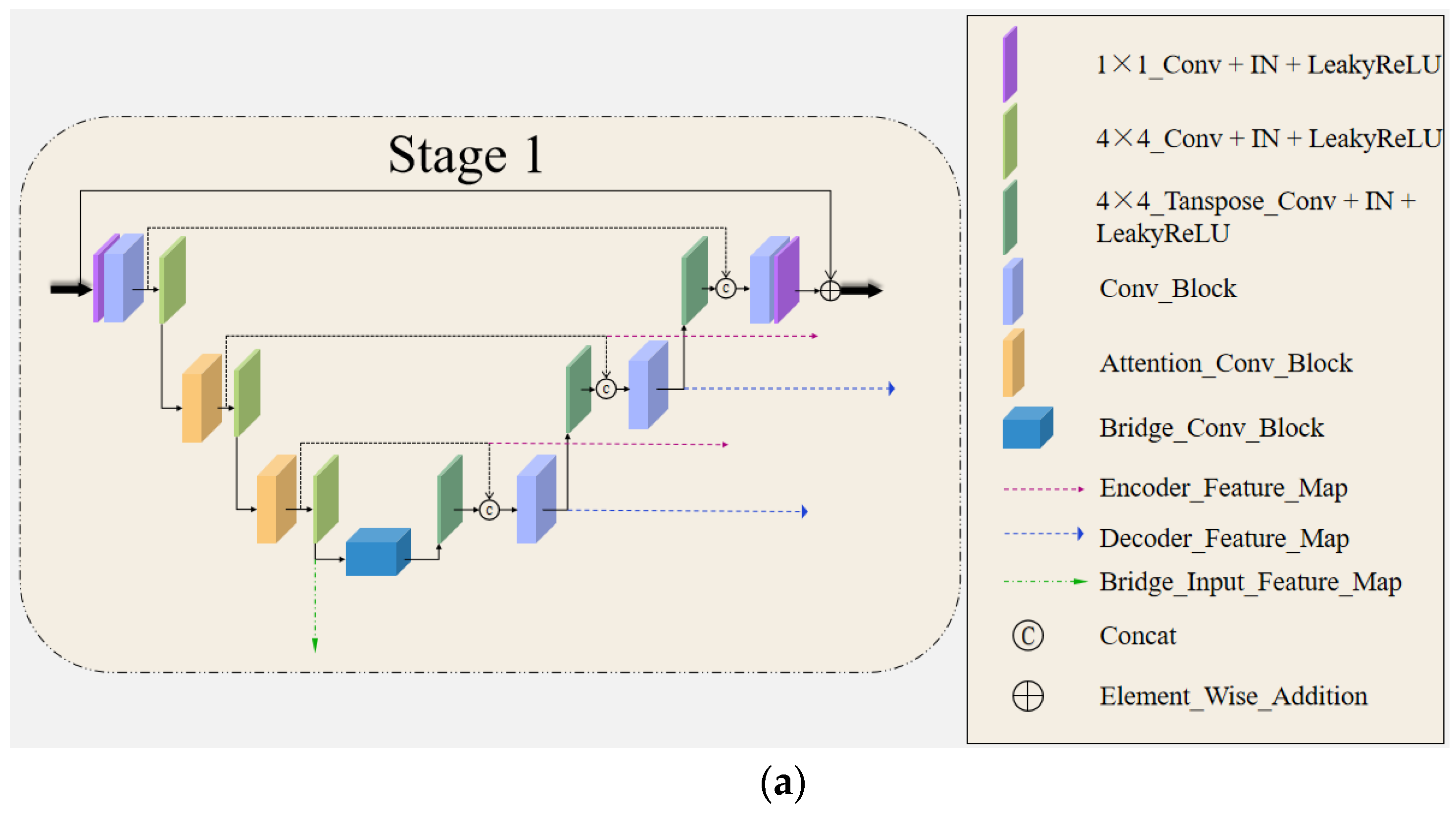
Our overall reconstruction network consists of three sub-networks to reconstruct high-quality MR images from undersampled images in three stages. The three sub-networks all adopt the encoder–decoder network structure, and also apply the microcosmic feature compensation connection inside the network. The three networks are roughly the same, but there are some differences in some details, as shown in Figure 2.
3.1.1. Stage One
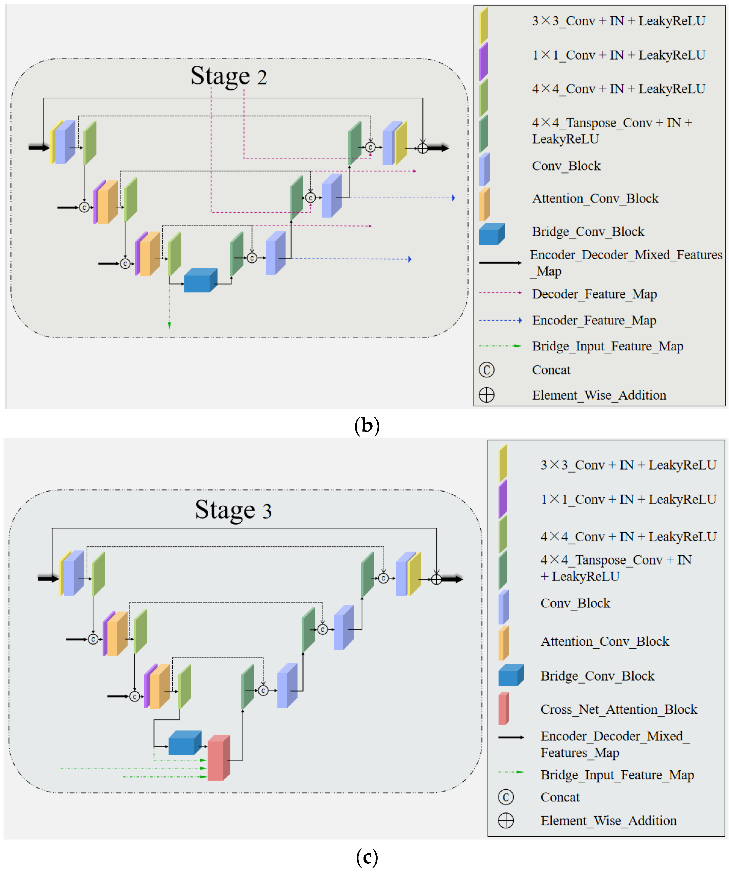
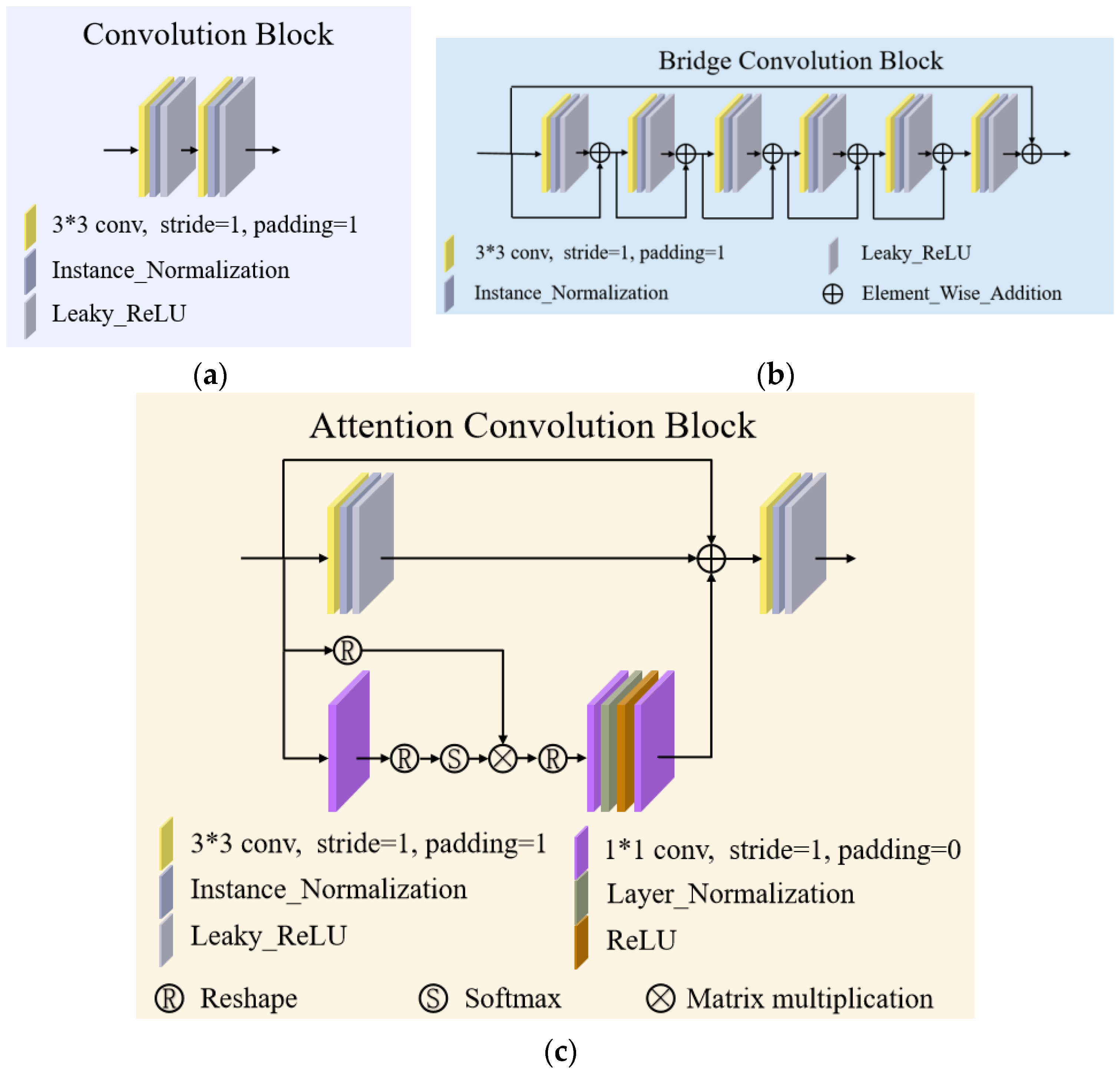
We use a network with an encoder and decoder structure, and the input image size is B × C × H × W. B stands for batch size, C stands for channel, H stands for image height, and W stands for image width. We take the real part and the imaginary part of the image on two channels for processing. This is because the collected k-space data is complex, and if the real part and the imaginary part are combined at the beginning, a lot of information will be lost. First, the input channel is changed from 2 to 32 through a 1 × 1 convolution layer, instance normalization (IN), and leakyReLU. Then the features are sent to the convolution block. The structure is shown in Figure 3a. This structure consists of two groups of 3 × 3 convolution, IN, and leakyReLU. The features of the image are extracted by a convolution operation. Note that the number of channels is kept constant here. After that, it will be down sampled by strided convolution. There is no pooling operation here. Strided convolution can make the network occupy less memory during training.
- Attention Convolution Block (ACB)
As shown in Figure 3c, here we design a module that combines attention with convolution. Convolution operation can extract image features, but this feature extraction is only limited to the size of the convolution kernel. Thus, the well-known disadvantage of convolution operation is that the receptive field is too small. Many researchers have tried to expand the convolution kernel size from 3 × 3 to 5 × 5 or even 7 × 7 and 9 × 9. However, this will increase a huge number of parameters, and the effect is not obvious. Based on GC block [28], we designed an attention convolution block to extract MRI image features more efficiently.
As shown in Figure 3c, we assume that the input feature map is x and its size is (B, C, H, W). This structure has four input branches, and we call the top-down branches the first, second, third, and fourth branches. We use to represent the transformation matrix of the first 3 × 3 convolution in the second branch, LR to represent the leakyReLU operation, and IN to represent the instance normalization operation, so the output of the second branch is
For the third branch, we first reshape it into a matrix of (B, 1, C, H × W) and get . For the fourth branch, we use to represent the transformation matrix of the first 1 × 1 convolution, and the number of output channels becomes 1. Then it is reshaped into (B, 1, H × W, 1) and we get .
After that, through softmax operation, matrix multiplication is performed with the data of the third branch to obtain , which is
Here, n is the number of positions in the feature map, where N = H × W. After the above operation, the matrix of (B, 1, C, 1) is obtained. Then we reshape it into (B, C, 1, 1) and note it as .
We use and to represent the next two 1 × 1 convolution transformation matrices, and LN to represent the layer normalization operation, so the final output of the third and fourth branches is
Then we make element-wise addition to the data of these branches. We use to represent the transformation matrix of the last 3 × 3 convolution, and the final output is:
That is the total of the operations of the attention convolution block. The processing unit improves the GC block by adding a convolution branch. So, we can combine the attention mechanism with convolution, and extract global and local features at the same time. Finally, we fuse the global features and local features to better encode the input data and enhance the network coding ability.
- Bridge Convolution Block (BCB)
The connection between encoder and decoder is called the bridge layer. Here, we use the bridge convolution block, which is a set of dense residual convolution layers. With its small size and low computation, the feature map of the bridge layer is suitable for complex convolution operations. Moreover, the semantic information of the bottom feature map is the most abstract, so it is necessary to extract more features. Based on the above analysis, we use this dense residual convolution structure to fully extract the information from the feature map. The specific structure is shown in Figure 3b.
3.1.2. Stage Two
As shown in Figure 2b, the sub-network in the second stage is roughly the same as that in the first stage. We replaced the 1 × 1 convolution at the beginning and the end with a 3 × 3 convolution. In addition, at the beginning of each layer of the encoder, 1 × 1 convolution, IN layer, and leakyReLU layer are introduced to fuse the features of the previous stage. It can be noted that compared with the first stage, the encoder and decoder here apply more feature compensation, which will be explained later in the introduction of the inter-stage feature compensation structure (IFCS).
3.1.3. Stage Three
As shown in Figure 2c, the sub-network of the third stage is roughly the same as that of the second stage. Compared with the previous two-stage network, this network does not need to transmit features to the later network. In addition, the cross network attention block (CNAB) is introduced here, and the specific operation of this structure is introduced in detail later.
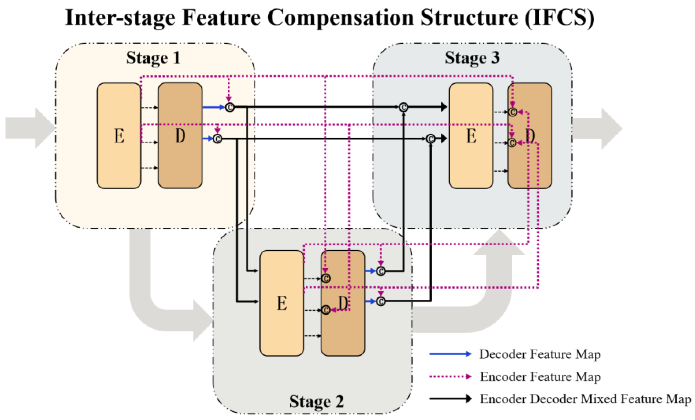
3.2. Inter-Stage Feature Compensation Structure (IFCS)
To effectively utilize the feature information of each sub-network, we designed an inter-stage feature compensation structure (IFCS). This structure is inspired by the internal skip connection of the U-Net network. According to our analysis, the internal feature compensation structure of the U-Net network is of great reference value. This structure compensates for the features of the encoder to the decoder, thus making the decoding stage more efficient. The downsampling operation in the encoding stage will lose a lot of spatial information, and this feature compensation in the network can make up for the lost information in the decoding stage. Meanwhile, the semantic information of encoder and decoder is usually different. By combining them, the semantic space of the decoding stage can be enriched, and the network decoding ability can be enhanced. This kind of structure is limited to the inside of the network, so we name the microscopic feature the compensation structure. Based on this idea, we extend it between networks from a macro point of view. That is to say, if each sub-network is compared to the encoder or decoder in the U-Net network, then similar feature compensation can be extended between networks.
The overall structure is shown in Figure 4. Let us first consider the decoder part. U-Net enhances the network decoding ability by compensating for the features of the encoder. We use the encoder features of the previous network to compensate for the decoder. Specifically, we compensate the encoder features of the first stage to the decoder parts of the second and third stages and compensate the encoder features of the second stage to the decoder part of the third stage. In this way, the decoder of the current network can not only integrate the encoder characteristics of the current network but also integrate the encoder characteristics of all previous networks. It enriches the semantic information of the decoder and makes up for the lost spatial information between networks. This stage of the network contains the encoder information of the previous stages, which expands the receptive field of the network to a certain extent and enables the network to capture global information.
Based on the above ideas, we focus on the encoder. We believe that the same idea can also be applied to the encoder to enhance the encoding ability of the network. We creatively mix the encoder and decoder information of the previous network and then compensate the mixed features to the encoder of the current network. Specifically, we mix the encoder features and decoder features of the first stage, and then compensate to the encoder parts of the second and third stages. Then, the encoder features and decoder features of the second stage are mixed and compensated to the encoder part of the third stage. In this way, the network encoding capability is greatly improved, and the encoder has the receptive field of the previous network. At the same time, we creatively compensate for the features of the previous network decoder to the current network encoder. This can enable the encoder to have a richer encoding space and to make up for the information lost in the previous stage of network decoding.
Experiments show that the design improves the network coding and decoding ability. It is an efficient and concise design, which greatly improves the network performance without introducing too much calculation.
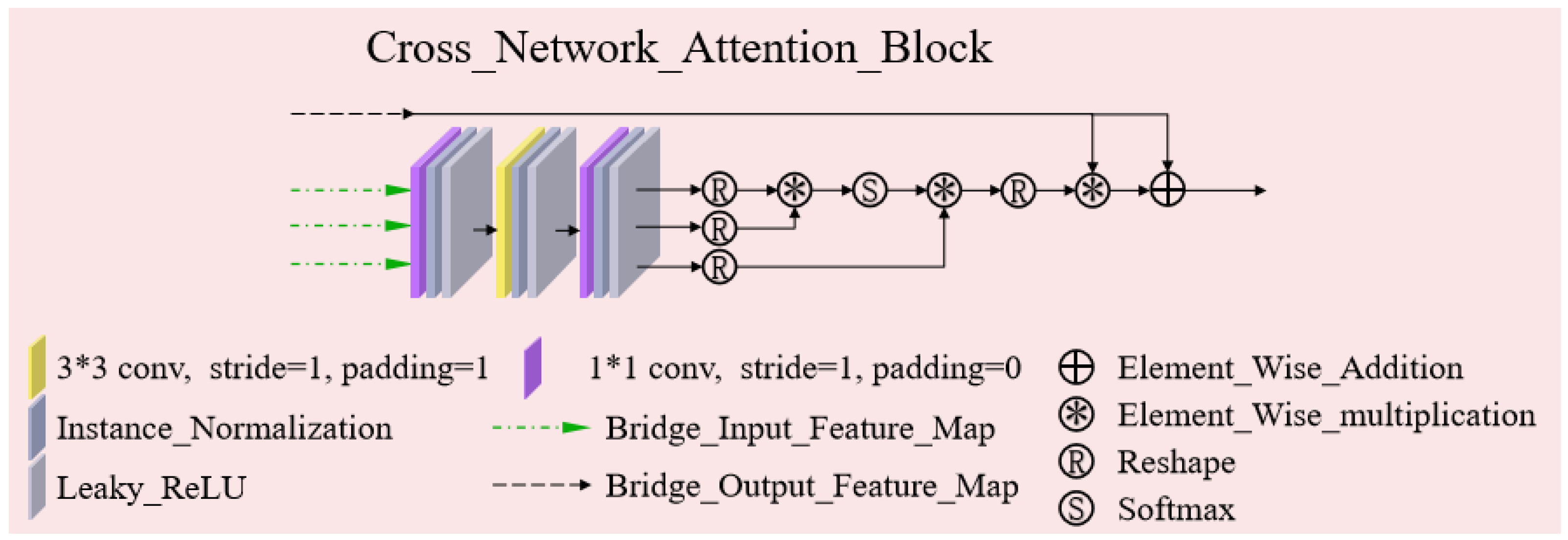
3.3. Cross Network Attention Block (CNAB)
To make more effective use of the underlying feature information between networks, we designed a cross network attention block (CNAB) for the bottom bridge layer. The specific structure is shown in Figure 5, and the green lines are the input features from three sub-network bridge layers. We send these features into a set of convolution layers with shared weights and obtain three output features. Suppose the three input features are , and , respectively, and the transformation matrix of the convolution layer is . After the convolution layer, we can get three output features with the channel number of 1, and we reshape them into features with the size of (B, C, H × W). After that, through matrix multiplication, softmax, and other operations, the attention feature map is obtained. Then, the attention feature map is multiplied and added with the output feature y of the third sub-network bridge layer. We express the final output as z. The whole operation process is shown in the following formula (the reshape operation is omitted in the formula):
Here, N = H × W indicates the number of positions in the feature map. Through this cross-network attention mechanism, we can obtain the feature information of the previous network and expand the receptive field to the whole world. Moreover, the bottom image has a small size and a low amount of computation, so the processing efficiency is very high. We fuse the features across the network and calculate the attention map and the feature map containing attention information is applied to the reconstruction network in the last stage. Our attention mechanism is no longer limited to the inside of the network but extends between the networks.
3.4. Data Consistency Module
We apply the data consistency module behind each sub-network, which plays a vital role in the cascaded network. The data consistency module is used to improve the fidelity of data and impose the constraint of the original MR measurement on the reconstruction data. We use soft DC here [29]:
where represents the set of index values of sampled data, represents the k-space data after network reconstruction, and represents the original real k-space data. is a trainable hyper-parameter, which is used to dynamically adjust the weights of the predicted data and the original k-space data. As shown in the above Formula (9), if the location point of k-space data is sampled, that is, it is in the set , then the value at this location will be replaced by the combination of the predicted value and the true value. If the location point of the k-space is not sampled, it is filled with the predicted value.
4. Implementation and Experiments
4.1. Dataset
Our method is tested on the fastMRI dataset [30]. In the field of machine learning, large public data sets are usually used for annual competitions and benchmark tests. The research of MR image reconstruction is usually trained and verified on several small, isolated datasets. This makes it difficult to compare the performance of different methods fairly. To solve this problem, Facebook and New York University jointly produced the fastMRI dataset [30]. This dataset is specially used for image reconstruction of machine learning technology, including original MRI k-space data and DICOM images. k-space data includes 1594 measurement datasets obtained from a series of MRI systems and clinical patient groups’ knee joint MRI examinations, and corresponding images derived from k-space data using the reference image reconstruction algorithm [20,30]. The test data released by this dataset only contains incomplete k-space matrixes and undersampled images. Note that the complete original k-space matrix here is the ground truth used in our reconstruction task. The ground truth (complete k-space matrix) of the test data has not been released. We need to upload the reconstructed image correctly before we can observe the test results and the corresponding rankings in the public ranking [18].
Our method was evaluated on the fastMRI single-coil knee joint [20] dataset. This data set contains original k-space data and DICOM images. The dataset consists of multiple volumes, and the number of slices in each volume is different, about 36. The training set, verification set, and test set consist of 973, 199, and 108 volumes. The ground truth of the test set has not been publicly released.
In the dataset we used, the undersampled images of the training sets and the validation sets are all in 4× acceleration mode. The undersampling mask includes a fully sampled central area, which accounts for 8% of all k-space lines. The rest positions are uniformly and randomly undersampled to obtain the required acceleration factor on average.
4.2. Loss Function
The output image of the network is expressed as Y, and the ground truth is X. Our training strategy is to supervise the output of the network in the image domain with ground truth. The SSIM index is mainly used to measure the structural similarity of two images, and the specific calculation method is given by [30]. The most important and meaningful thing in MR images is the structural information, so our reconstruction task is to make the output image as similar as possible to the ground truth in structure. Based on the above considerations, the loss function is defined as follows:
4.3. Implementation Details
The proposed method is implemented with PyTorch framework and is tested on two NVIDIA Tesla V100 GPUs. We trained 50 epochs in total, and the initial learning rate was 0.001, which became 0.0001 at the 40th epoch. We use RMSProp optimizer to optimize the network.
We use average structural similarity (SSIM), peak signal to noise ratio (PSNR), and normalized mean square error (NMSE) to measure the quality of the reconstructed image [31]. The image performance and evaluating indicators on the test set can be seen on the fastMRI single-coil knee public leader board [18].
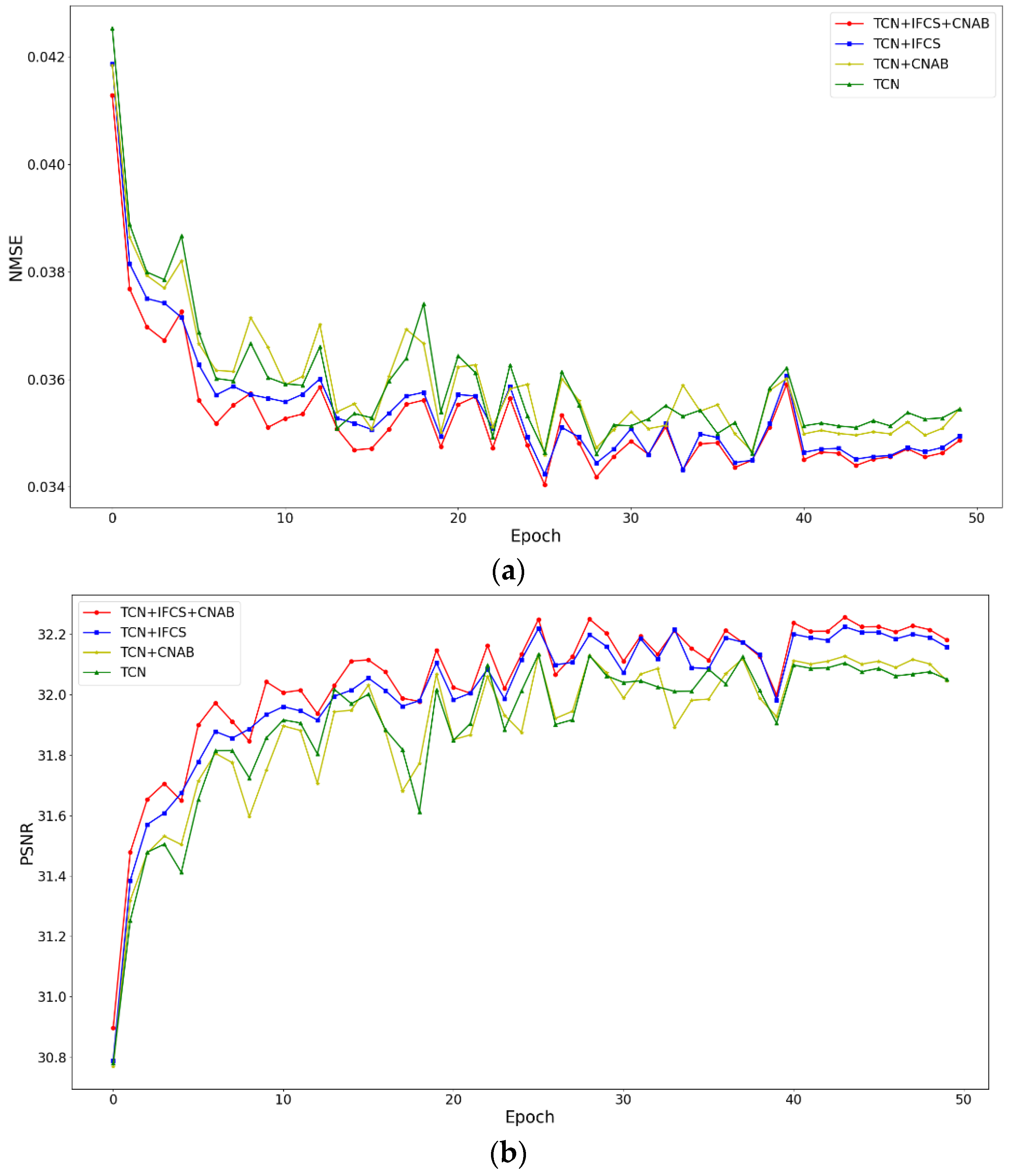
4.4. Ablation Study
The DMFF-Net, excluding inter-stage feature compensation structure (IFCS) and cross network attention block (CNAB), is called the triple convolution network (TCN). DMFF-Net is TCN+IFCS+CNAB. We verify the effectiveness of the proposed TCN, IFCS, and CNAB through several ablation experiments, and the experimental results are shown in Table 1. Here, we take U-Net as the baseline for the comparative experiment. Because our DMFF-Net contains three stages of sub-networks, we also cascaded U-Net three times for fair comparison. A soft DC layer is also added behind its sub-network, and the cascaded network is called U-Net_cascade3. Our ablation experiment and the comparison experiment with the baseline network were conducted on the validation set, and the experimental results are shown in Table 2.
As can be seen from Table 2, the performance of our TCN network is already better than that of U-Net and U-Net_cascade3. Our complete network DMFF-Net has much better performance than U-Net and U-Net_cascade3. No matter whether NMSE, PSNR, or SSIM, our DMFF-Net has achieved the best results. It can be seen from Table 1 that our three-stage sub-network is very effective in the reconstruction task, and it also proves the effectiveness of processing units. From the experimental results, it can be seen that the proposed IFCS is very effective, obviously improves the quality of reconstruction, and plays a key role in the network. Our designed CNAB further improves the network performance. Although the effect of the CNAB is not obvious when acting alone, it can give full play to its advantages when cooperating with IFCS.
4.5. Comparisons with State-of-the-Art Methods
We compared our method with the TV Model [20], KIKI-Net [21], MD-Recon-Net [22], U-Net Baseline Model [20], XPDNet [23], and i-RIM [24] on the test set data of fastMRI data set. In addition, we also compared DMFF-Net with MD-Recon-Net, U-Net Baseline Model, and KIKI-Net in the validation set, because the codes of these networks are all available.
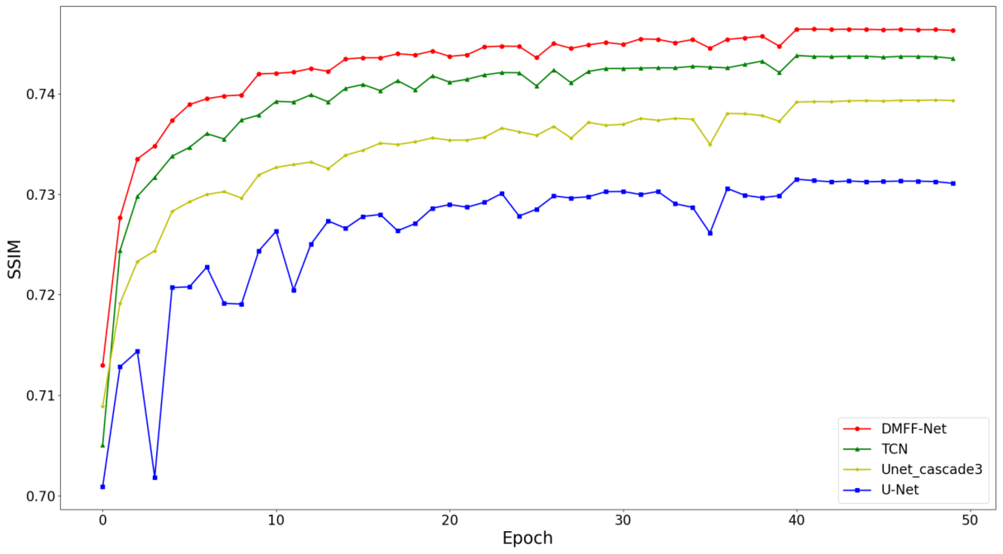
4.5.1. Comparisons on Validation Set
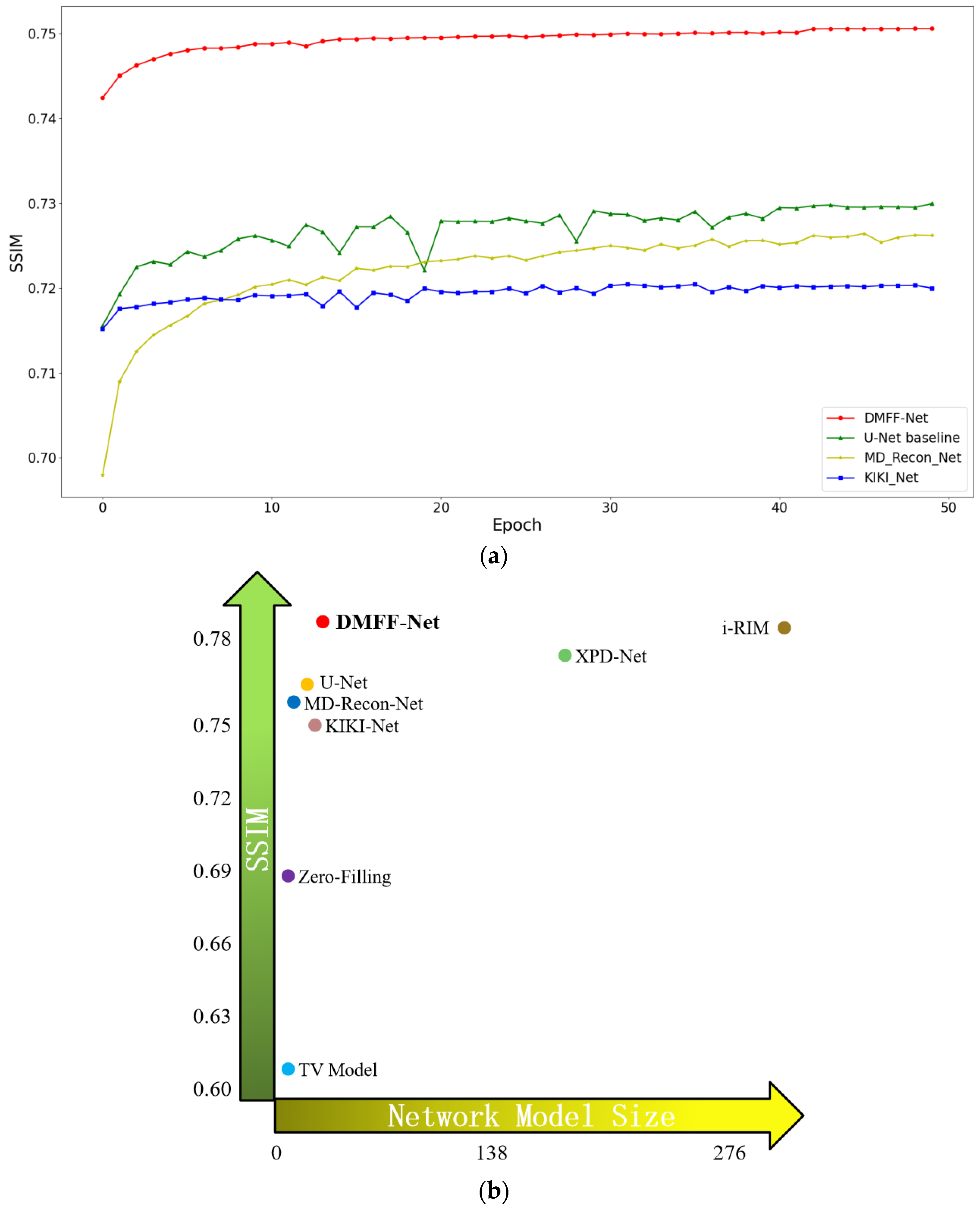
As shown in Figure 8a, the reconstruction performances of DMFF-Net, MD-Recon-Net, U-Net Baseline Model, and KIKI-Net on the validation set are shown here. It can be seen intuitively from the figure that from the first epoch to the last epoch, the SSIM of our DMFF-Net is always significantly higher than that of other methods. This result fully reflects the advantages and effectiveness of our method. Specifically, the SSIM values of DMFF-Net, MD-Recon-Net, U-Net Baseline Model, and KIKI-Net are 0.7506, 0.7262, 0.7299, and 0.7199, respectively.
4.5.2. Comparisons on Test Set
As mentioned earlier, the test set of the fastMRI data set has not released the ground truth. We need to upload the reconstruction results of the test set to the leaderboard [18] to see our reconstruction results. We also achieved a competitive ranking on the leaderboard. In the following, we mainly compare Zero Filling, TV Model [20], KIKI-Net [21], MD-Recon-Net [22], U-Net Baseline Model [20], XPD-Net [23], i-RIM [24], and our DMFF-Net methods from the perspective of SSIM. As shown in Table 3, our DMFF-Net has achieved the best performance. It can be found that the performance of the i-RIM method here is also very high. However, it should be noted that the parameter of this network is 275 M, while our DMFF-Net parameter is only 18.7 M. Therefore, our network has achieved both lightweight and very high performance. XPD-Net is very prominent in these networks, and its NMSE and PSNR are the best. The SSIM of XPD-Net does not perform very well, and its parameters are large, which will cause a lot of computation.
In Figure 8b, we drew the curve of the relationship between SSIM and model size (i.e., model parameters). Here, the very left of the horizontal axis represents the smallest model size, and the very top of the vertical axis represents the best SSIM performance. Therefore, the closer to the upper left corner of the coordinate plane, the more ideal is the model. It can be seen intuitively that our model is the best among these algorithms. DMFF-Net achieved very high SSIM performance with relatively small model size, and we achieved the best balance between reconstruction quality and model size.
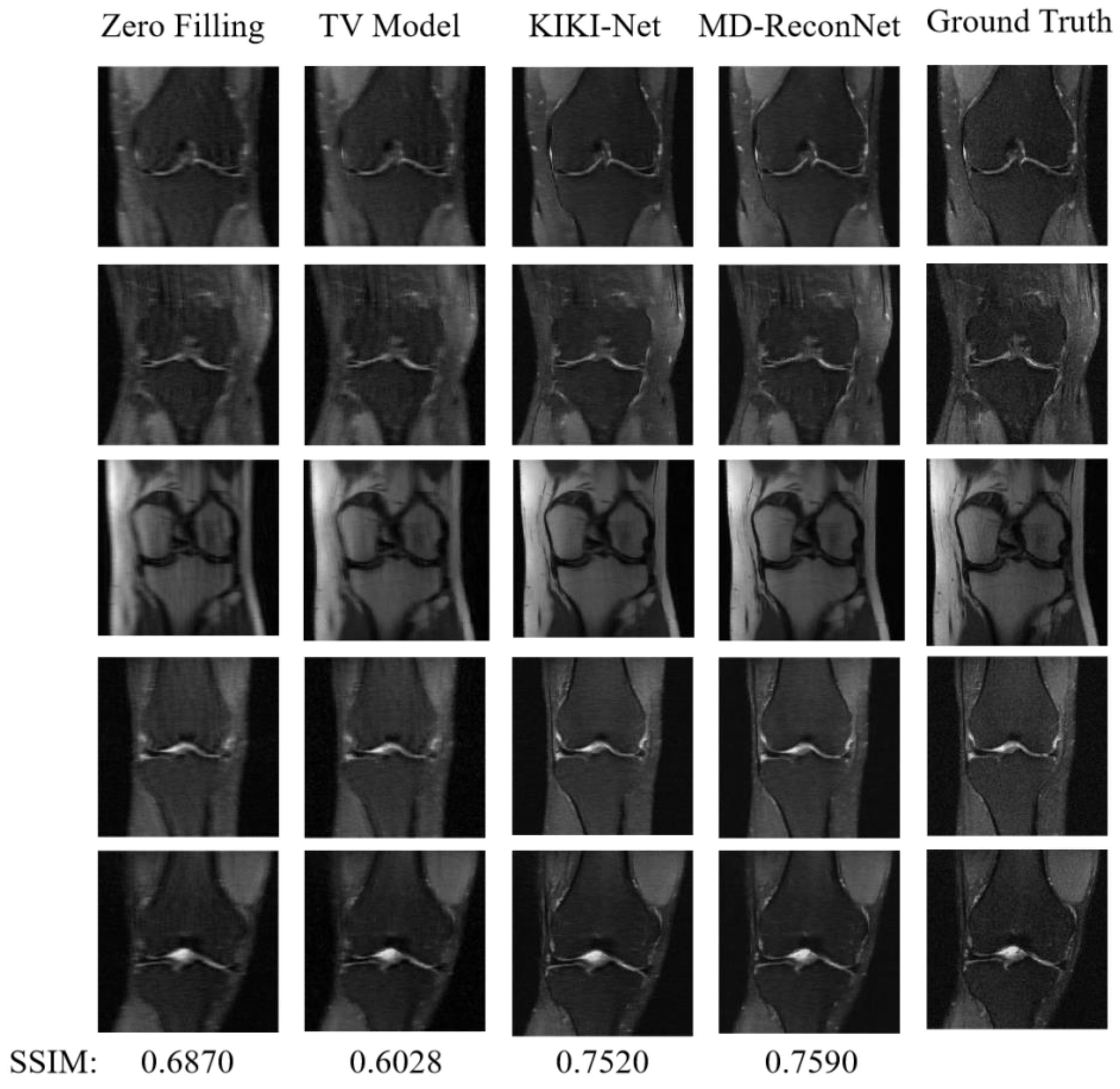
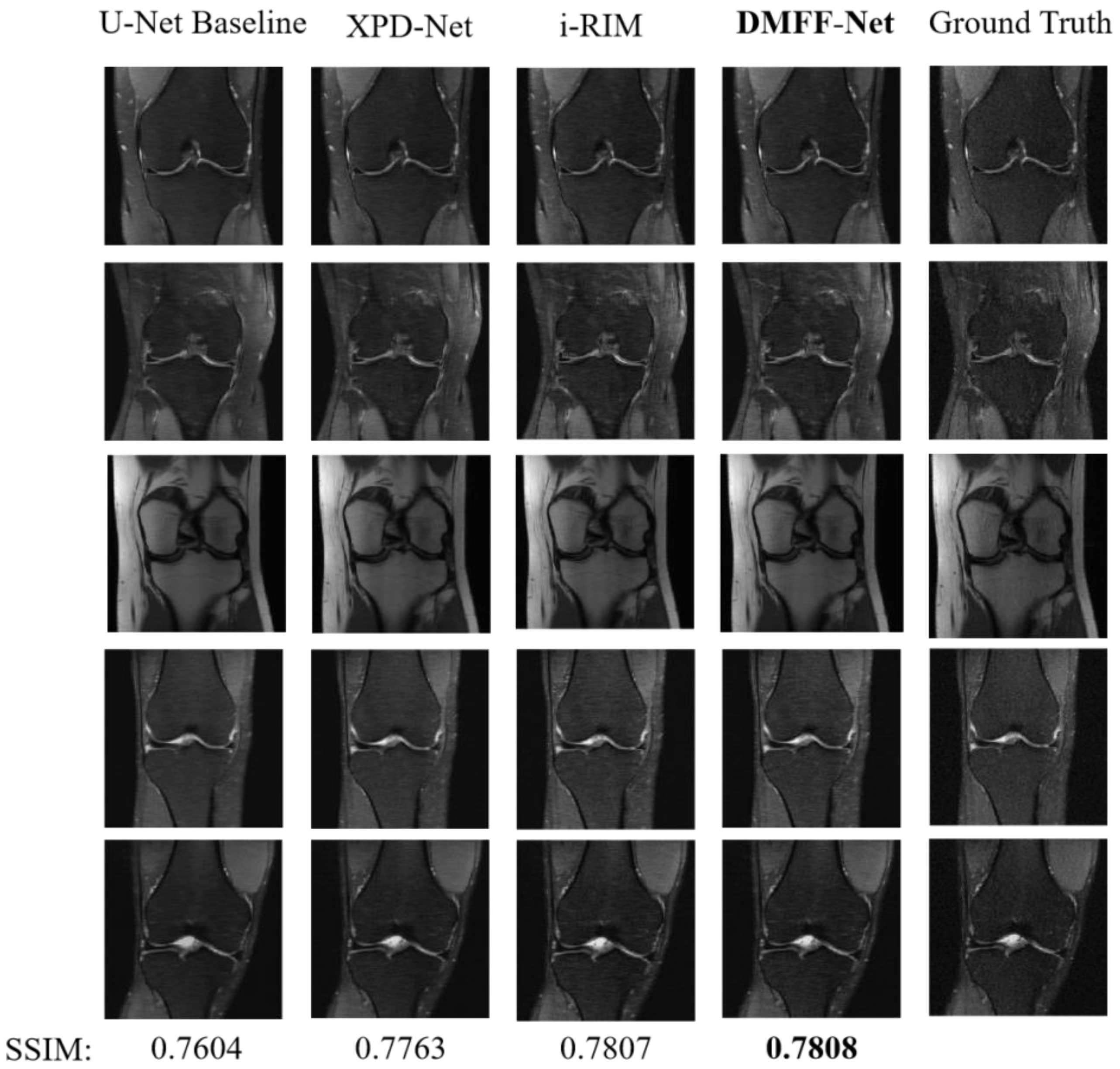
To observe the effect of each network reconstruction more intuitively, we placed the reconstruction results of these networks in Figure 9. It can be seen from Figure 9 that the effect of the Zero Filling and TV Model is worse than that of deep learning. The reconstruction effect of U-Net is better than KIKI-Net and MD-Recon-Net, and it can suppress artifacts in images better. However, the U-Net baseline has the disadvantage of over-smoothing, and it is easy to lose detailed information. XPD-Net, i-RIM, and DMFF-Net have not only achieved outstanding effects in suppressing artifacts but also kept the high-frequency information of images well, showing more detailed textures. Among them, our DMFF-Net is superior to XPD-Net and i-RIM.
5. Discussion and Conclusions
In this paper, we rethought the feature utilization methods in the U-Net network from a macro perspective and proposed a DMFF-Net network for MR image reconstruction. We used the reconstruction strategy of a triple-stage sub-network to reconstruct high-quality MR images from undersampled images from coarse to fine. We extended the skip connection feature compensation of U-Net from inside the network to between the networks and introduced the feature compensation mechanism of the encoder. Using the dual feature compensation and cross-stage feature compensation of the encoder and decoder, we proposed the inter-stage feature compensation structure (IFCS), which fuses features in a densely macroscopic way between sub-networks and significantly improves the network encoding and decoding ability. Inspired by the self-attention mechanism, we put forward the cross network attention block (CNAB) to further improve the quality of reconstructed images.
To verify the effectiveness of our method, we designed some comparative experiments. We conducted experiments on the fastMRI dataset and uploaded the results to the fastMRI single-coil knee public leader board [18] published by Facebook. It can be seen from the specific data that the final performance of zero filling method is only 0.6870, while that of TV-model method is only 0.6028. However, the performance of our method reached 0.7808, which is a great improvement of about 10%. Compared with the current advanced methods, such as KIKI-Net (0.7520), MD-Recon-Net (0.7590), and U-Net Baseline (0.7604), our method achieved nearly 3% performance improvement. For the XPD-Net and i-RIM methods with high performance, although our performance is not much improved, our parameters are very small in comparison. Our parameters are only 18.7 M, which is 6.7–14.3% of those of the two methods. This means that the computation for our method is very small, and the reconstruction speed is greatly improved. The experimental results show that our method can effectively remove the artifacts in the image, and fully retain the structural details. Compared with other networks, our method is not only lightweight, but also can achieve very high performance.
Author Contributions
Z.S. was responsible for proposing ideas, designing networks, writing and revising papers, and conducting experiments. Y.S. was responsible for making suggestions and supervision. X.L. was responsible for making suggestions and providing experimental data. Y.P. was responsible for proposing ideas, making suggestions, supervising and revising papers. All authors have read and agreed to the published version of the manuscript.
Funding
The authors gratefully acknowledge the financial supports by the National Natural Science Foundation of China under Grant numbers 52227814.
Data Availability Statement
The data can be obtained on the official website of FastMRI, with the address of https://fastmri.org/dataset/ (accessed on 3 November 2022).
Acknowledgments
We would like to thank Jin Ruiqi and Liu Yiming for their suggestions in writing the paper.
Conflicts of Interest
The authors declare no conflict of interest.
References
- Pal, A.; Rathi, Y. A review of deep learning methods for MRI reconstruction. arXiv 2021, arXiv:2109.08618. [Google Scholar]
- Liu, Y.; Leong, A.T.; Zhao, Y.; Xiao, L.; Mak, H.K.; Tsang, A.C.; Lau, G.K.; Leung, G.K.; Wu, E.X. A low-cost and shielding-free ultra-low-field brain MRI scanner. Nat. Commun. 2021, 12, 7238. [Google Scholar] [CrossRef]
- Donoho, D.L. Compressed Sensing. IEEE Trans. Inf. Theory 2006, 52, 1289–1306. [Google Scholar] [CrossRef]
- Sodickson, D.K. Spatial encoding using multiple RF coils: SMASH imaging and parallel MRI. In Methods in Biomedical Magnetic Resonance Imaging and Spectroscopy; John Wiley & Sons Ltd.: Chichester, UK, 2000; pp. 239–250. [Google Scholar] [CrossRef]
- Griswold, M.A.; Jakob, P.M.; Heidemann, R.M.; Nittka, M.; Jellus, V.; Wang, J.; Kiefer, B.; Haase, A. Generalized Autocalibrating Partially Parallel Acquisitions (GRAPPA). Magn. Reson. Med. 2002, 47, 1202–1210. [Google Scholar] [CrossRef] [PubMed] [Green Version]
- Pruessmann, K.P.; Weiger, M.; Scheidegger, M.B.; Boesiger, P. SENSE: Sensitivity encoding for fast MRI. Magn. Reason. Med. 1999, 42, 952–962. [Google Scholar] [CrossRef]
- Wang, S.; Xiao, T.; Liu, Q.; Zheng, H. Deep Learning for Fast MR Imaging: A Review for Learning Reconstruction from Incomplete K-space Data. Biomed. Signal Process. Control 2021, 68, 102579. [Google Scholar] [CrossRef]
- Varoquaux, G.; Cheplygina, V. Machine learning for medical imaging: Methodological failures and recommendations for the future. npj Digit. Med. 2022, 5, 48. [Google Scholar] [CrossRef]
- Protonotarios, N.E.; Katsamenis, I.; Sykiotis, S.; Dikaios, N.; Kastis, G.A.; Chatziioannou, S.N.; Doulamis, A. A few-shot U-Net deep learning model for lung cancer lesion segmentation via PET/CT imaging. Biomed. Phys. Eng. Express 2022, 8, 025019. [Google Scholar] [CrossRef]
- Kawauchi, K.; Furuya, S.; Hirata, K.; Katoh, C.; Manabe, O.; Kobayashi, K.; Shiga, T. A convolutional neural network-based system to classify patients using FDG PET/CT examinations. BMC Cancer 2020, 20, 227. [Google Scholar] [CrossRef] [Green Version]
- Kumar, A.; Fulham, M.; Feng, D.; Kim, J. Co-learning feature fusion maps from PET-CT images of lung cancer. IEEE Trans. Med. Imaging 2019, 39, 204–217. [Google Scholar] [CrossRef]
- Arabi, H.; AkhavanAllaf, A.; Sanaat, A.; Shiri, I.; Zaidi, H. The promise of artificial intelligence and deep learning in PET and SPECT imaging. Phys. Med. 2021, 83, 122–137. [Google Scholar] [CrossRef]
- Cho, C.; Lee, Y.H.; Park, J.; Lee, S. A Self-Spatial Adaptive Weighting Based U-Net for Image Segmentation. Electronics 2021, 10, 348. [Google Scholar] [CrossRef]
- Ronneberger, O.; Fischer, P.; Brox, T. U-Net: Convolutional Networks for Biomedical Image Segmentation. In Proceedings of the International Conference on Medical Image Computing and Computer-Assisted Intervention, Munich, Germany, 5–9 October 2015; Springer: Berlin/Heidelberg, Germany, 2015; pp. 234–241. [Google Scholar]
- Ibtehaz, N.; Rahman, M.S. MultiResUNet: Rethinking the U-Net Architecture for Multimodal Biomedical Image Segmentation. Neural Netw. 2020, 121, 74–87. [Google Scholar] [CrossRef]
- Jha, D.; Smedsrud, P.H.; Riegler, M.A.; Johansen, D.; Lange, T.D.; Halvorsen, P.; Johansen, H.D. ResUNet++: An Advanced Architecture for Medical Image Segmentation. In Proceedings of the 2019 IEEE International Symposium on Multimedia, San Diego, CA, USA, 9–11 December 2019; pp. 225–2255. [Google Scholar]
- Zhou, Z.; Siddiquee, M.M.R.; Tajbakhsh, N.; Liang, J. UNet++: Redesigning Skip Connections to Exploit Multiscale Features in Image Segmentation. IEEE Trans. Med. Imaging 2020, 39, 1856–1867. [Google Scholar] [CrossRef] [Green Version]
- Facebook AI, NYU Langone Health. FastMRI Single-Coil Knee Public Leader Board. Available online: https://fastmri.org/leaderboards/ (accessed on 3 November 2022).
- Xie, Y.; Li, Q. A Review of Deep Learning Methods for Compressed Sensing Image Reconstruction and Its Medical Applications. Electronics 2022, 11, 586. [Google Scholar] [CrossRef]
- Zbontar, J.; Knoll, F.; Sriram, A.; Murrell, T.; Huang, Z.; Muckley, M.J.; Defazio, A.; Stern, R.; Johnson, P.; Bruno, M.; et al. FastMRI: An Open Dataset and Benchmarks for Accelerated MRI. arXiv 2018, arXiv:1811.08839. [Google Scholar]
- Eo, T.; Jun, Y.; Kim, T.; Jang, J.; Lee, H.; Hwang, D. KIKI-net: Cross-domain Convolutional Neural Networks for Reconstructing Undersampled Magnetic Resonance Images. Magn. Reason. Med. 2018, 80, 2188–2201. [Google Scholar] [CrossRef]
- Ran, M.; Xia, W.; Huang, Y.; Lu, Z.; Bao, P.; Liu, Y.; Sun, H.; Zhou, J.; Zhang, Y. MD-Recon-Net: A Parallel Dual-Domain Convolutional Neural Network for Compressed Sensing MRI. IEEE Trans. Radiat. Plasma Med. Sci. 2021, 5, 120–135. [Google Scholar] [CrossRef]
- Ramzi, Z.; Ciuciu, P.; Starck, J.L. XPDNet for MRI Reconstruction: An Application to the 2020 FastMRI Challenge. arXiv 2020, arXiv:2010.07290. [Google Scholar]
- Putzky, P.; Karkalousos, D.; Teuwen, J.; Miriakov, N.; Bakker, B.; Caan, M.; Welling, M. I-RIM Applied to the FastMRI Challenge. arXiv 2019, arXiv:1910.08952. [Google Scholar]
- Wang, X.; Girshick, R.; Gupta, A.; He, K. Non-Local Neural Networks. In Proceedings of the 2018 IEEE/CVF Conference on Computer Vision and Pattern Recognition, Salt Lake City, UT, USA, 18–23 June 2018; pp. 7794–7803. [Google Scholar]
- Vaswani, A.; Shazeer, N.; Parmar, N.; Uszkoreit, J.; Jones, L.; Gomez, A.N.; Kaiser, Ł.; Polosukhin, I. Attention Is All You Need. In Proceedings of the 31st Conference on Neural Information Processing Systems, Long Beach, CA, USA, 4–9 December 2017; pp. 5998–6008. [Google Scholar]
- Hu, J.; Shen, L.; Albanie, S.; Sun, G.; Wu, E. Squeeze-and-Excitation Networks. IEEE Trans. Pattern Anal. Mach. Intell. 2020, 42, 2011–2023. [Google Scholar] [CrossRef] [PubMed] [Green Version]
- Cao, Y.; Xu, J.; Lin, S.; Wei, F.; Hu, H. GCNet: Non-Local Networks Meet Squeeze-Excitation Networks and Beyond. In Proceedings of the 2019 IEEE/CVF International Conference on Computer Vision Workshop, Seoul, Republic of Korea, 27–28 October 2019; pp. 1971–1980. [Google Scholar]
- Sriram, A.; Zbontar, J.; Murrell, T.; Defazio, A.; Zitnick, C.L.; Yakubova, N.; Knoll, F.; Johnson, P. End-to-End Variational Networks for Accelerated MRI Reconstruction. In Proceedings of the Medical Image Computing and Computer Assisted Intervention; Martel, A.L., Abolmaesumi, P., Stoyanov, D., Mateus, D., Zuluaga, M.A., Zhou, S.K., Racoceanu, D., Jos-kowicz, L., Eds.; Springer International Publishing: Cham, Switzerland, 2020; pp. 64–73. [Google Scholar]
- Wang, Z.; Bovik, A.C.; Sheikh, H.R.; Simoncelli, E.P. Image Quality Assessment: From Error Visibility to Structural Similarity. IEEE Trans. Image Process. 2004, 13, 600–612. [Google Scholar] [CrossRef] [PubMed] [Green Version]
- Knoll, F.; Zbontar, J.; Sriram, A.; Muckley, M.J.; Bruno, M.; Defazio, A.; Parente, M.; Geras, K.J.; Katsnelson, J.; Chandarana, H.; et al. FastMRI: A Publicly Available Raw k-Space and DICOM Dataset of Knee Images for Accelerated MR Image Reconstruction Using Machine Learning. Radiol. Artif. Intell. 2020, 2, e190007. [Google Scholar] [CrossRef] [PubMed]
Figure 1.
Overview of the DMFF-Net. The network consists of three stages. The internal structure of each stage is the same, but there are some differences in details. We make use of the microscopic features compensation structure within the stage and the macroscopic features compensation structure between the stages. The feature compensation between stages covers the features of encoder and decoder and is used to enhance the encoding and decoding capability in the later stage.

Figure 2.
Three-stage sub-network. (a) The network structure of the first stage. (b) The network structure of the second stage. (c) The network structure of the third stage. The sub-network structure of these three stages is roughly the same, but there are some differences in details. We reconstruct high-quality MR images from undersampled images from coarse to fine through a three-stage network.


Figure 3.
Some network modules. (a) The convolution block. (b) The bridge convolution block. (c) The attention convolution block (ACB). We applied the above processing units in the three-stage network.
Figure 3.
Some network modules. (a) The convolution block. (b) The bridge convolution block. (c) The attention convolution block (ACB). We applied the above processing units in the three-stage network.

Figure 4.
Inter-stage feature compensation structure (IFCS). The figure describes the IFCS structure used in this network, which is a structure for feature compensation between networks from a macro perspective. In the figure, pink lines represent encoder features, blue lines represent decoder features, and black thick lines represent encoder–decoder hybrid features.

Figure 5.
Cross network attention block (CNAB). This is an attention mechanism that uses the feature information between networks to calculate.
Figure 5.
Cross network attention block (CNAB). This is an attention mechanism that uses the feature information between networks to calculate.

Figure 6.
Results of ablation experiment. Used to observe the effectiveness of our proposed structure. (a) Comparison results between NMSE. (b) Comparison results between PSNR. (c) Comparison results between SSIM.
Figure 6.
Results of ablation experiment. Used to observe the effectiveness of our proposed structure. (a) Comparison results between NMSE. (b) Comparison results between PSNR. (c) Comparison results between SSIM.


Figure 7.
Experimental results compared with the baseline network.

Figure 8.
Compared with other state-of-the-art methods. (a) Comparisons on validation set. (b) Comparisons on validation set and the relationship between SSIM and model size.
Figure 8.
Compared with other state-of-the-art methods. (a) Comparisons on validation set. (b) Comparisons on validation set and the relationship between SSIM and model size.

Figure 9.
The reconstruction results of several methods, the end right of which is the ground truth, available at the public leaderboard of fastMRI [18].
Figure 9.
The reconstruction results of several methods, the end right of which is the ground truth, available at the public leaderboard of fastMRI [18].


Table 1.
Ablation experiment. Here we mainly observe the role of each module in our network. IFCS represents inter-stage feature compensation structure, CNAB represents cross network attention block. TCN represents the DMFF-Net excluding IFCS and CNAB. √ indicates that this part is included in the network used in this experiment.
| TCN | IFCS | CNAB | NMSE | PSNR | SSIM |
|---|---|---|---|---|---|
| √ | 0.03545 | 32.05 | 0.7435 | ||
| √ | √ | 0.03494 | 32.16 | 0.7457 | |
| √ | √ | 0.03545 | 32.05 | 0.7442 | |
| √ | √ | √ | 0.03486 | 32.18 | 0.7463 |
Table 2.
Comparison to baseline network. Here we mainly observe the performance comparison between the complete network and the baseline network.
Table 2.
Comparison to baseline network. Here we mainly observe the performance comparison between the complete network and the baseline network.
| NMSE | PSNR | SSIM | |
|---|---|---|---|
| U-Net | 0.03828 | 31.39 | 0.7313 |
| U-Net_cascade3 | 0.03599 | 31.92 | 0.7393 |
| TCN | 0.03545 | 32.05 | 0.7435 |
| DMFF-Net | 0.03486 | 32.18 | 0.7463 |
Table 3.
Comparisons with state-of-the-art methods on the test set.
| Parameters | NMSE | PSNR | SSIM | |
|---|---|---|---|---|
| Zero Filling | -- | 0.0438 | 30.5 | 0.6870 |
| TV-Model [20] | -- | 0.0479 | 30.7 | 0.6028 |
| KIKI-Net [21] | 1.25 M | 0.0296 | 32.8 | 0.7520 |
| MD-Recon-Net [22] | 0.3 M | 0.0272 | 33.3 | 0.7590 |
| U-Net Baseline [20] | 7.8 M | 0.0271 | 33.2 | 0.7604 |
| XPD-Net [23] | 155 M | 0.0251 | 33.9 | 0.7763 |
| i-RIM [24] | 275 M | 0.0271 | 33.7 | 0.7807 |
| DMFF-Net | 18.7 M | 0.0271 | 33.7 | 0.7808 |
Publisher’s Note: MDPI stays neutral with regard to jurisdictional claims in published maps and institutional affiliations. |
© 2022 by the authors. Licensee MDPI, Basel, Switzerland. This article is an open access article distributed under the terms and conditions of the Creative Commons Attribution (CC BY) license (https://creativecommons.org/licenses/by/4.0/).
Share and Cite
MDPI and ACS Style
Sun, Z.; Pang, Y.; Sun, Y.; Liu, X. DMFF-Net: Densely Macroscopic Feature Fusion Network for Fast Magnetic Resonance Image Reconstruction. Electronics 2022, 11, 3862. https://doi.org/10.3390/electronics11233862
AMA Style
Sun Z, Pang Y, Sun Y, Liu X. DMFF-Net: Densely Macroscopic Feature Fusion Network for Fast Magnetic Resonance Image Reconstruction. Electronics. 2022; 11(23):3862. https://doi.org/10.3390/electronics11233862
Chicago/Turabian StyleSun, Zhicheng, Yanwei Pang, Yong Sun, and Xiaohan Liu. 2022. "DMFF-Net: Densely Macroscopic Feature Fusion Network for Fast Magnetic Resonance Image Reconstruction" Electronics 11, no. 23: 3862. https://doi.org/10.3390/electronics11233862
Note that from the first issue of 2016, this journal uses article numbers instead of page numbers. See further details here.