

Research on a Random Route-Planning Method Based on the Fusion of the A* Algorithm and Dynamic Window Method


School of Biological and Chemical Engineering, Zhejiang University of Science and Technology, Hangzhou 310023, China
*
Author to whom correspondence should be addressed.
Electronics 2022, 11(17), 2683; https://doi.org/10.3390/electronics11172683
Submission received: 14 July 2022
/
Revised: 17 August 2022
/
Accepted: 23 August 2022
/
Published: 26 August 2022
(This article belongs to the Special Issue Feature Papers in Electrical and Autonomous Vehicles)
Abstract
:Path planning is a hot topic at present. Considering the global and local path planning of mobile robot is one of the challenging research topics. The objective of this paper is to create a rasterized environment that optimizes the planning of multiple paths and solves barrier avoidance issues. Combining the A* algorithm with the dynamic window method, a robo-assisted random barrier avoidance method is used to resolve the issues caused by collisions and path failures. Improving the A* algorithm requires analyzing and optimizing its evaluation function to increase search efficiency. The redundant point removal strategy is then presented. The dynamic window method is utilized for local planning between each pair of adjacent nodes. This method guarantees that random obstacles are avoided in real-time based on the globally optimal path. The experiment demonstrates that the enhanced A* algorithm reduces the average path length and computation time when compared to the traditional A* algorithm. After fusing the dynamic window method, the local path is corrected using the global path, and the resolution for random barrier avoidance is visualized.
1. Introduction
Path planning aims to solve robot movement problems along the optimal route from the starting point to the destination. Since the invention of the robot, path planning has become a central focus of robot research [1,2]. Multiple attempts have been made by scientists to find a collision-free path for the moving robot. This type of research is extremely important because it enables robots to quickly complete tasks without human guidance. Various researchers have utilized optimization criteria to endow robots with self-awareness. In recent years, the A* algorithm [3,4], the D* algorithm [5], and the ant colony have been used to represent global planning as well as the artificial potential field in robot path planning research. The DWA is responsible for local planning. Global and local path planning [6] differ in their knowledge of the environment variable information of a mobile robot.
Global path planning refers to the robot planning a safe, collision-free optimal path in a known static environment to establish an accurate global map in advance. Global path planning is extensively employed in the shipping industry [7,8], agriculture [9], aerospace [10], autonomous driving [11], and other fields and constitutes an important research topic. To overcome the limitations of traditional ant colony algorithm in indoor mobile robot path planning, such as long path planning time, slow convergence speed, nonoptimal path, and local optimal solution, Miao et al. [12] proposed an improved adaptive ant colony algorithm. Sandamur et al. [13] proposed a whole-area traversal path planning algorithm for orchards; the maximum area coverage rate of the proposed algorithm is 76%. Huang et al. [14] proposed a rotary-wing drone operation path planning algorithm for multi-area and complex boundary fields. They employed polygon grouping to distinguish blocks of different shapes. Combined with route sorting and heading optimization, flight trajectory can be obtained quickly. Zhang et al. [15] developed a strategy for automatic path planning by using the automatic identification system (AIS) data and simple round unit (SRU), where the ship routes and velocity were generated by extracting the correlations among ship routes by using the AIS tracking data. To better address ship path planning in the virtual 3D context, Xie et al. [16] formulated a 2.5D navigation graph technique for achieving walking domain modeling, as well as a modified A* algorithm for planning large ship paths. By fusing the A* and ant colony algorithms, Lan et al. [17] developed a modified algorithm for path planning, resolving the limitations of the ant colony algorithm, such as numerous iterations, slow convergence, and long search duration in global path planning, as well as ready trapping into the local optimization in an intricate environment. Li et al. [18] proposed a multi-way A* algorithm that enables valid and real-time 3D path planning of autonomous underwater vehicles, reduces the number of search nodes, and enables further search path reduction. A hybrid mapping-based framework for global path planning was established by Wang et al. [19]. The global path was estimated from the scene diagram and mapped to the lower level, and then the geometric path was generated. Given the generation of a high level from a low level, the generated global path offers powerful guidance for measurement path computation. The A* algorithm has a short planning path and quick computing rate. It is now a common approach for global route planning [20]. In local path planning, the Artificial potential field and dynamic window methods have gained widespread application popularity. Wang Zhi [21] combined the A* algorithm and the improved artificial potential field method for realizing random obstacle avoidance in a complex environment; however, the path based on the artificial potential field method appears less smooth.
However, in the aforementioned studies, obstacles absent in the previous map could not be considered in global path planning [22,23]. Accordingly, local path planning, which allows real-time path generation based on the sensor information, was applied. In local path planning, when random obstacles exist in the environment in which the robot is located [24,25], the robot can avoid them according to the real-time observation information obtained from the sensor so that the robot can safely reach the target point. By expanding VO, Berg et al. [26] achieved smooth path planning without vibrations. Xu et al. [27] proposed VO, where the obstacle velocities exceeding the maximum robotic velocity were considered. Howard et al. [28,29] proposed a state lattice planner (SLP) that utilizes the constraint and state datasets of robots for candidate path generation. However, in the presence of barriers in the robot’s periphery, candidate path generation cannot be realized using SLP. Being a simple strategy, the dynamic window approach enables smooth path planning and avoidance of local obstacles [30]. The dynamic window method is proposed by Fox [31]. This algorithm samples the various velocities contained within the velocity space of the robotic kinematics model. In addition, it simulates robot trajectories within a given time frame and scores the simulated trajectories according to a variety of scoring rules. DWA is extensively employed in path planning and current ROS (Robot Operating Systems). Since different robots have different shapes, their path-planning approaches and strategies in the same environment depend on their shapes and sizes [32]. Zhang et al. [33] proposed an enhanced DWA that uses stereoscopic vision to avoid obstacles, and the optimal speed of the robot was achieved by defining a strict search space. As stereo vision increases the complexity of time and space, however, a few minor localized issues can still occur. For better path optimization, Dobrevski et al. introduced deep reinforcement learning and DWA into local path planning [34]. By integrating DWA and the jump-A* algorithm, Liu et al. [35] proposed a global dynamic path planning method. However, the candidate paths produced by DWA, where the velocities are hypothesized to be fixed for a certain duration, are linear and arc-shaped [36]. Given the failure to consider barriers in the foregoing candidate paths, they are inappropriate for application in narrow spaces. Li et al. [37] proposed an enhanced DWA that takes into account the free space relationship between the dimensions of the mobile robot and the obstacles, but it is susceptible to local optimality. Vista et al. [38] proposed an enhanced DWA to make its objective function convergent but failed to fully account for the environment. The current DWA continues to have the following problems: Dynamic constraints only account for the acceleration limitations of the robot's driving power. The effects of the vehicle's vertical loads and road imperfections on acceleration are disregarded. The calculation of the trajectory is optimal only when considering the errors caused by the car's actual walk. The dynamic window method's strengths include a simple model, a smooth planning path, and an advantageous local obstacle avoidance ability [39]. Wang et al. [40] and colleagues proposed using the dynamic window method for local planning between the two nodes of the A* algorithm, which has a smooth driving trajectory and good random obstacle avoidance ability, but the search efficiency of A* algorithm must be enhanced. Many studies are currently being conducted to enhance the search efficiency of the A* algorithm. Based on the dynamic path planning model developed by Li et al. [41], the invading submarine path was optimized using the ABC algorithm; this approach is feasible for planning the evasive path during the submarine search. Through collision simulation, Xu et al. [42] assessed the developed formula’s performance.
The paper presents a random obstacle avoidance method for robots that combines the improved A* algorithm and the dynamic window method in an effort to address the aforementioned issues. This method considers the path smoothness and the search efficiency of the A* algorithm. When the globally optimal path node is determined using the enhanced A* algorithm, the dynamic window method should be utilized for local path planning between each pair of adjacent nodes. Thus, if the mobile robot encounters random obstacles on the global path, it can avoid them and return to the global path. This not only ensures global path optimization but can also randomly avoid obstacles.
2. Improved A* Algorithm
In the field of path planning, the Dijkstra algorithm must be implemented. The A* algorithm is optimized compared to the Dijkstra algorithm and introduces an evaluation function to instruct node extension and search, thus improving the robot path planning efficiency [43].
The evaluation function for the traditional A* algorithm is:
means the path distance estimate for the robot at a node is the target function for the A* algorithm. refers to the distance loss of the robot during the movement from the starting position to the current position. Distance loss is measured using the formula as a known value. indicates that when the robot is moving from the current position to its intended target position during the course of its movement, the distance estimate of the robot will vary slightly according to the formula. As an essential step of the evaluation function for the A* algorithm, the distance estimate guarantees the accuracy and efficiency of the A* algorithm.
However, redundant collinear nodes and tangents exist on the path obtained by the conventional A* algorithm. If the robot follows such a path, its movement will become incoherent [44]. In order to address the aforementioned issues, the A* algorithm is enhanced in two ways: To increase the search efficiency of the A* algorithm, the improved search point selection strategy and the optimization of the heuristic function are presented first. Next, the redundant point deletion strategy is implemented to eliminate any redundant nodes to optimize the path. Therefore, the path consists of the starting point, the destination, and the pivotal turning point.
2.1. Optimize Search Point Selection Strategy
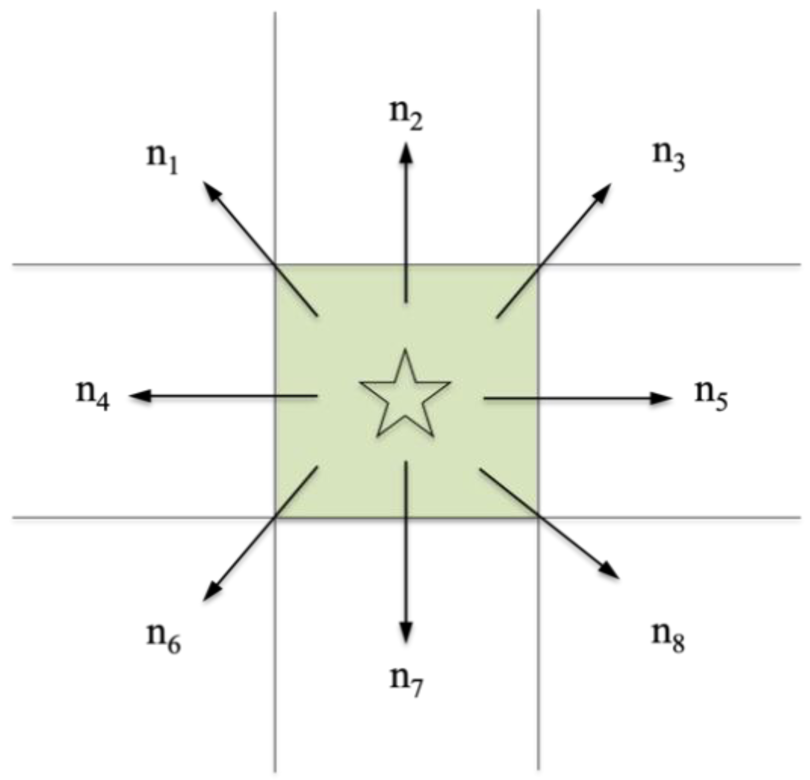
As shown in Figure 1, the dark grids are the current points, and n1 to n8 represent the eight moving directions in the current grid.
The limitation of the target point orientation results in unnecessary grids in eight of the neighboring grids, which wastes time and storage space during operation. This article proposes optimizing the search point selection strategy based on the relative position of the target point and the current point after discarding three of the search directions and reserving five of the search directions to increase the search efficiency [45]. First, the connection between the target point and the current point and the angle of the n direction are determined, then the correspondence between the corner and three of the abandoned directions is shown in Table 1.
With these optimizations, you can reduce the number of search nodes to increase computing efficiency.
2.2. Inspiration Function of Optimization Algorithm
Traditional A* algorithms search for paths by traversing numerous unnecessary nodes, which reduces search efficiency [46]. The primary contributor is the algorithm-inspired function design. If the estimated value for the inspirational function is less than the actual generation value, the search node becomes less efficient, but the optimal path can still be located. If the estimated value for the inspiration function is greater than the actual generation value, there are fewer and more efficient search nodes, and the optimal path is difficult to locate. The searching operation is most efficient when the estimated cost of the inspirational function equals the actual cost. Due to the European nature of the inspiration function, its value will never surpass the actual distance between the current point and the target point. If the current point is far from the target point, the estimated value for the inspiration function is significantly lower than the actual value, and the algorithm has multiple search nodes, resulting in low operational efficiency. As the current point approaches the target point, the estimate approaches the actual value more closely. In order to find the optimal path, it is necessary to reduce the estimated weight so that it is not excessive. In conclusion, the cost function is improved, as shown in (2).
Formula: represents the composite value; indicates the estimated proxy value from the current point to the target point; and represents the actual generation value from the starting point to the current point. represents the distance between the starting point and the destination, while represents the distance between the current point and the destination.
2.3. Redundant Point Removal Policy
While these enhancements improve the efficiency of the search, there are still numerous redundant and unnecessary points on the path that are incompatible with the following path of the robot. This paper proposes a policy to remove superfluous nodes while retaining only necessary branching points [47]. The specific redundancy point deletion policies are as follows: Initially, traverse each node in the path sequentially and remove the current node if it is on the same line as the front and back nodes. Second, after removing the redundant point on the same line, set the node in the path to , connect point P1 to point P3, and if the distance between the line segment P1P3 is greater than the safe distance, the barrier is erected. Connect point P1 to point P4 until the distance between P1Pk, and the barrier is less than the predetermined safe distance, then connect P1Pk−1, and remove the middle node. Iterate from point P2 until every path node has been traversed.
After redundant point removal policy operations, the A* algorithm-based path contains only the start, end, and necessary nodes, effectively reducing the path length.
3. Improved Dynamic Window Algorithm
The dynamic window method has been considered a local path planning algorithm for guiding robot movement. It is based on speed data collected during robot movement and a simulation of the robot's trajectory under speed drive [48]. Given the disadvantage of the traditional dynamic window method, which lacks the guidance of global programming, this paper improves the evaluation function of the dynamic window method by combining it with global path information. This ensures that the final partial programming matches the globally optimal path, thereby enhancing the local–optimal problem [49].
When planning the path, the dynamic window method first determines the range of robotic motion speed, then incorporates the range into the robotic motion model, simulates the trajectory, scores multiple trajectories using the evaluation function, and the trajectory with the highest fractional score is the optimal trajectory currently planned by the robot. The following steps are to establish the robot motion model, determine the robot velocity range, and determine the evaluation function.
3.1. Establishment of the Robot’s Motion Model
The dynamic window method simulates the trajectory through the robot motion model to find the best path among several simulated trajectories. Let be the robotic t-hour line velocity, be the t-hour angular velocity, and the position increment of the two adjacent moments be:
The position of the t + 1 moment is expressed as:
where the range of changes in the translation velocity is decided by the nearest distance to the obstacle as well as the maximum line reduction speed. Similarly, the range of rotation velocity depends on the nearest distance to the obstacle and the maximum angular deceleration.
3.2. Determination of the Robotic Velocity Range
The robot's speed relies on the maximum–minimum speed, motor performance, and braking distance of the robot. The robot has a maximum speed of:
The motor speed constraints are:
in: the current line speed is ; the current angular velocity is ; the maximum linear acceleration is ; the maximum angular acceleration is ; the maximum linear attenuation is ; and the maximum angular reduction speed is .
Brake distance constraint: to ensure the robot’s safety in case of a random obstruction, the robot must stop before hitting the obstruction:
where is the distance between the analog trajectory and the nearest obstacle. The three aforementioned constraints limit the speed range of the robot. The robotic speed range can be expressed as follows:
3.3. Improvement of the Evaluation Function
With the evaluation function, the optimal trajectory can be determined by simulating several trajectories in accordance with the motion velocity range and the robot motion model. This paper improves the evaluation function, combines it with global path information, and ensures that the final local path is based on the globally optimal path, as opposed to the traditional dynamic window method, which falls easily into local optimality. The enhanced evaluation function is displayed in Format (9).
in: means the angle of difference of the trajectory’s end direction with the current target point; suggests the distance between the trajectory and the nearest obstacle; represents the current velocity evaluation function; σ refers to a smooth function; α, β, γ are weighted coefficients. This evaluation function enables planning routes to prevent random obstacles, applicable to the globally optimal path.
However, the minimum distance value collected by the sensor is discrete and not continuous. Evaluation of the trajectory directly by using Equation (9) will result in errors. Therefore, the evaluation function expressed by Equation (9) must be further processed and normalized.
4. Simulation and Verification of the Robot Random Obstacle Avoidance Algorithm Based on an Improved A* Algorithm
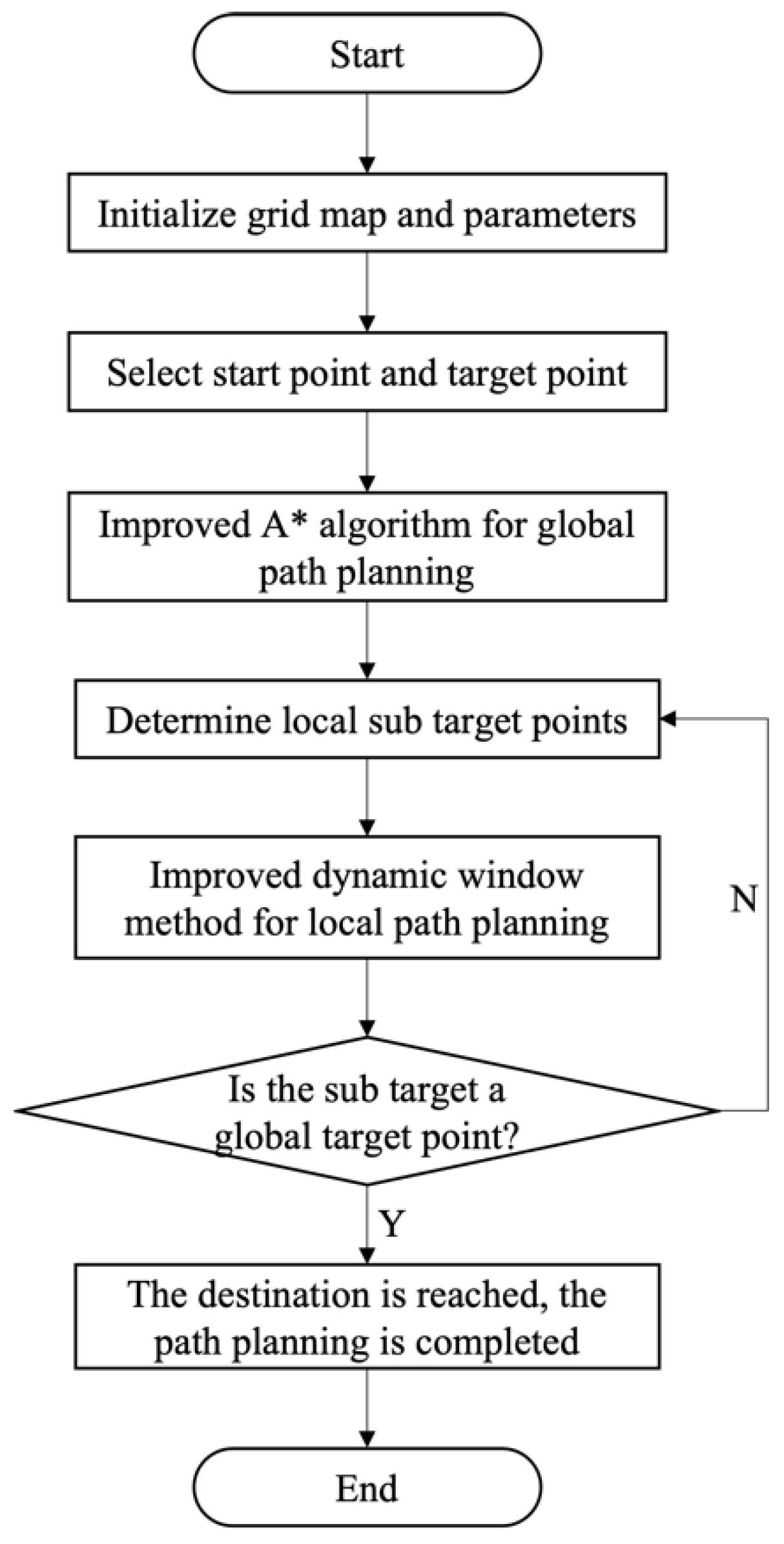
This paper incorporates the enhanced A* algorithm and the dynamic window method in order to achieve global path optimization and random obstacle avoidance. The particular steps are as follows: First, the global path is planned using the enhanced A* algorithm [50]. After determining the optimal global node sequence, the dynamic window method is utilized to plan the local path between each pair of adjacent nodes. This diagram illustrates the flow of the robot’s random obstacle avoidance algorithm based on an enhanced A* algorithm (Figure 2).
In this section, the improved algorithm will be simulated and validated to test the practicability and reliability of the A* algorithm fusion dynamic window method in a complex environment. The simulation experiments were conducted in the MATLAB 2017b software environment. The simulation results were used to test the effectiveness of the fusion algorithm.
4.1. The Experiment Analysis of an Improved A* Algorithm
The raster map was built in the form of 30 × 30 specification. During the simulation experiment, the starting position and target position of the robot in the raster map were kept constant. The starting position and the end point were, respectively, labeled as “S” and “T”. The obstacles and boundary positions in the raster map were fixed.
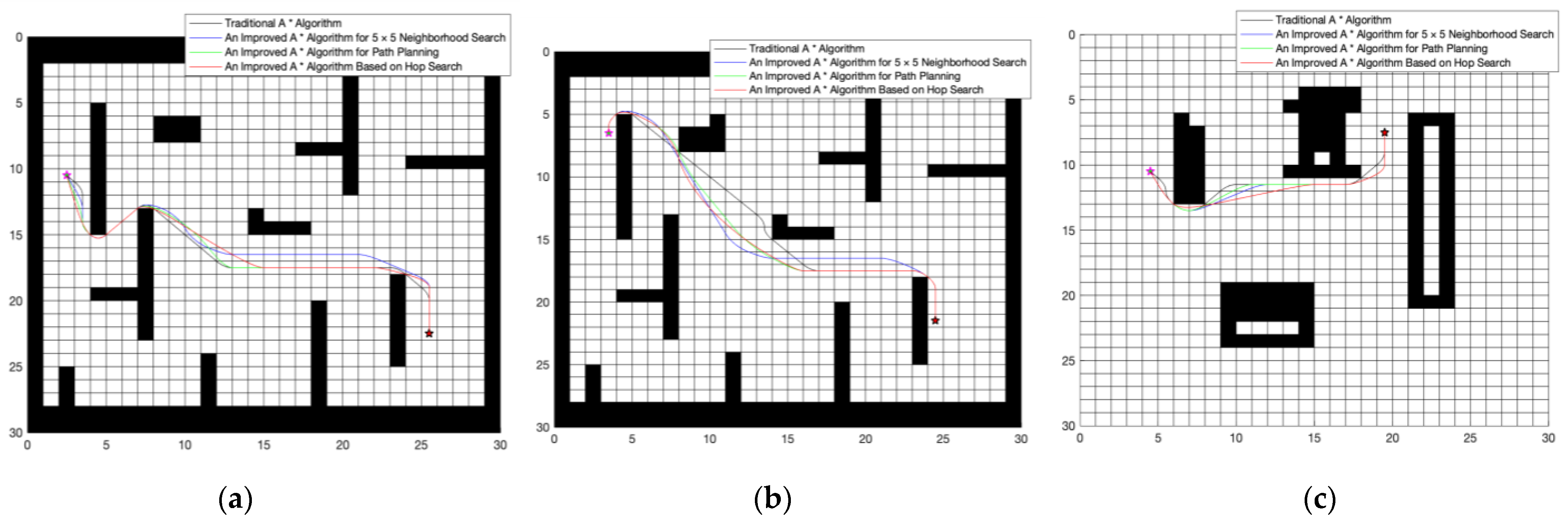
Path planning utilizes the improved A* algorithm with a 5 × 5 neighborhood, the improved A* algorithm based on the hop-point search method, and the improved A* algorithm. The optimization results are validated by altering the environmental data. Environment I is a 30 × 30 two-dimensional grid map with starting coordinates of S(3,11) and ending coordinates of T(26,23), barrier coverage of p = 20.7%, and path planning results are depicted in Figure 3a. Environment II is a 30 × 30 two-dimensional grid map with beginning coordinates of S(4,7) and ending coordinates of T(25,22), and barrier coverage of p = 21.3%. Figure 3b displays the results of path planning. Environment III is a 30 × 30 grid map with starting coordinates of S(5, 11), ending coordinates of T(20, 8), and barrier coverage of p = 10.5%. Figure 3c displays the results of path planning.
Table 2 shows the path regularization results for these four algorithms. According to the simulation experiments, the traditional A* algorithm, the improved A* algorithm with a 5 × 5 search neighborhood, the improved A* algorithm based on the hop-point search method, and the improved A* algorithm are used for global path planning in three environments. In terms of planning time, the improved A* algorithm can reduce average planning time by 21% compared to the traditional A* algorithm, whereas the improved A* algorithm based on the hop-point search is less than the improved A* algorithm based on 5 × 5 neighborhood. This is because the improved method in this paper reduces some search nodes compared to the traditional A* algorithm, the improved A* algorithm based on 5 × 5 neighborhood, and the improved method based on hop-point search. In terms of turning points, the improved A* algorithm can reduce the number of turning points in most cases. Overall, the path planned by the improved the A* algorithm in this paper has further improved and has higher search efficiency.
4.2. Analysis of Random Barrier Avoidance Effect of the Improved A* Algorithm Fusion Dynamic Window Method
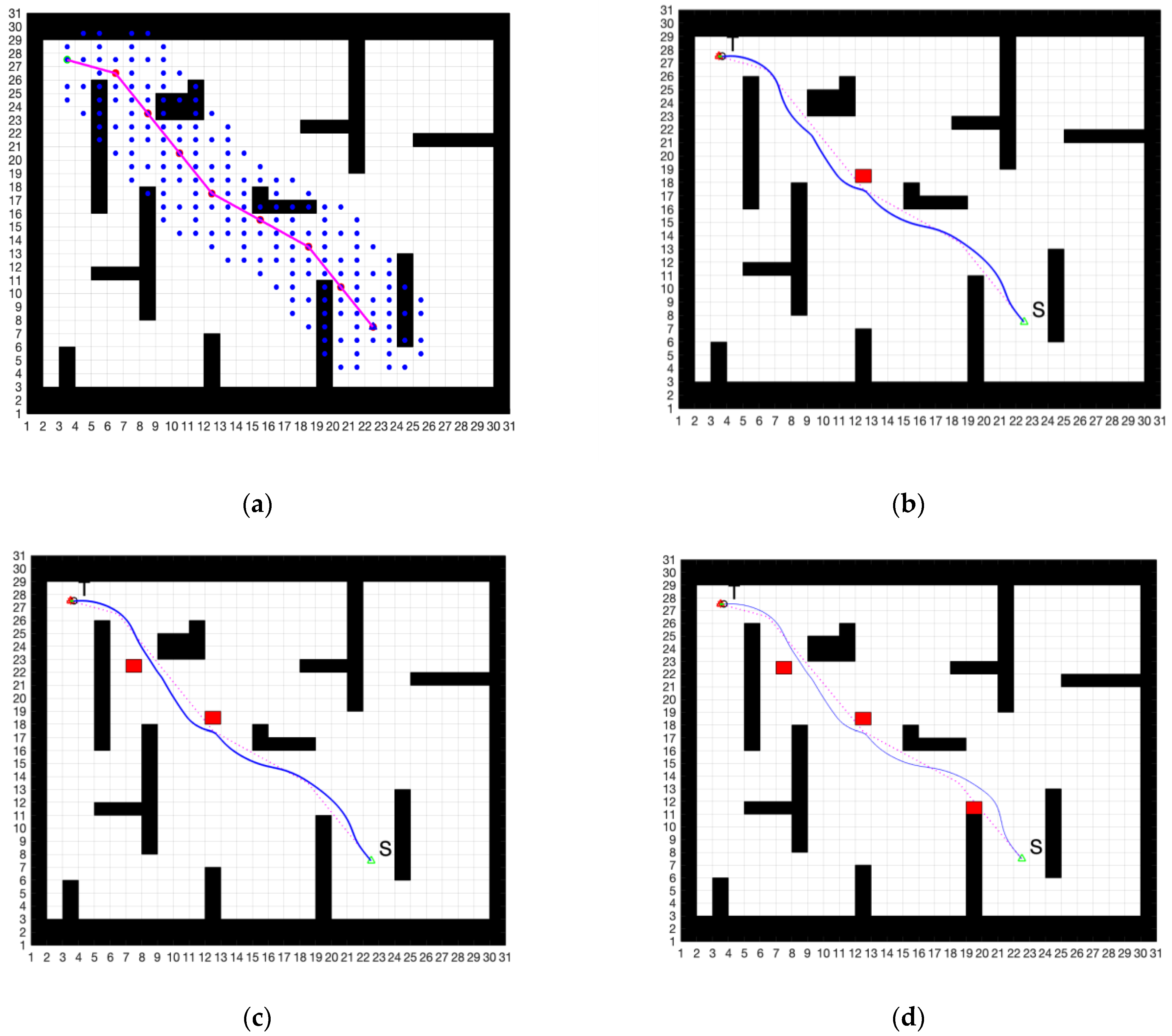
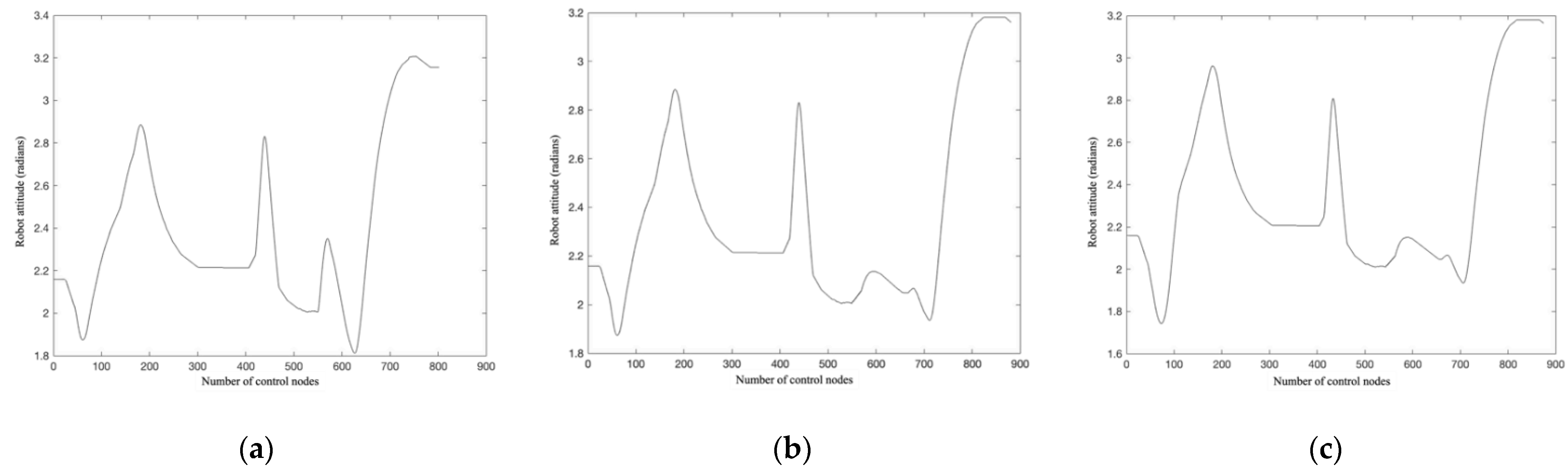
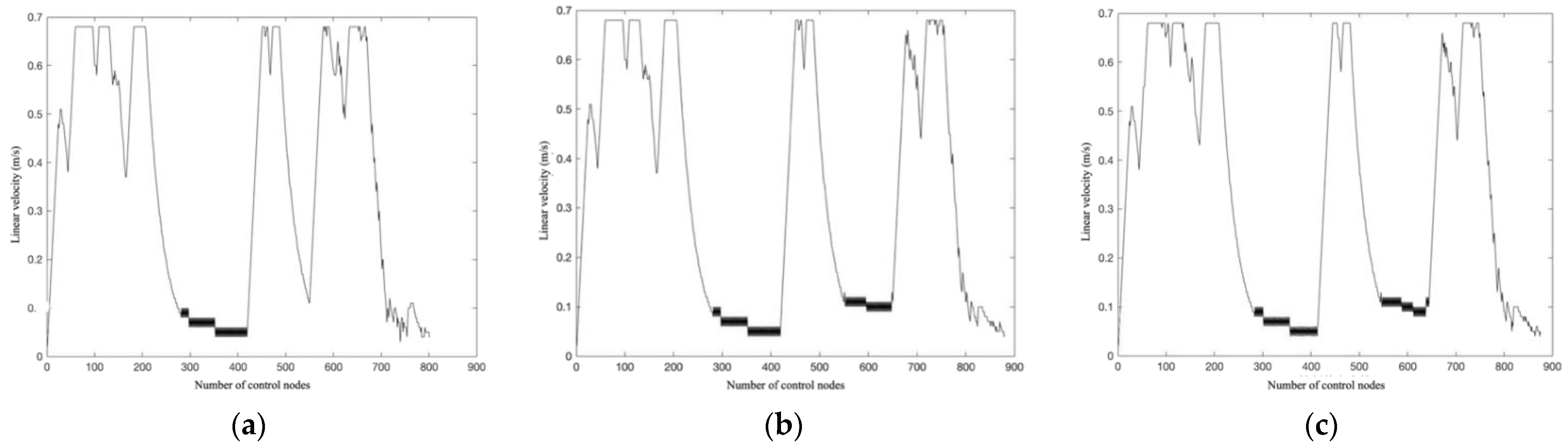
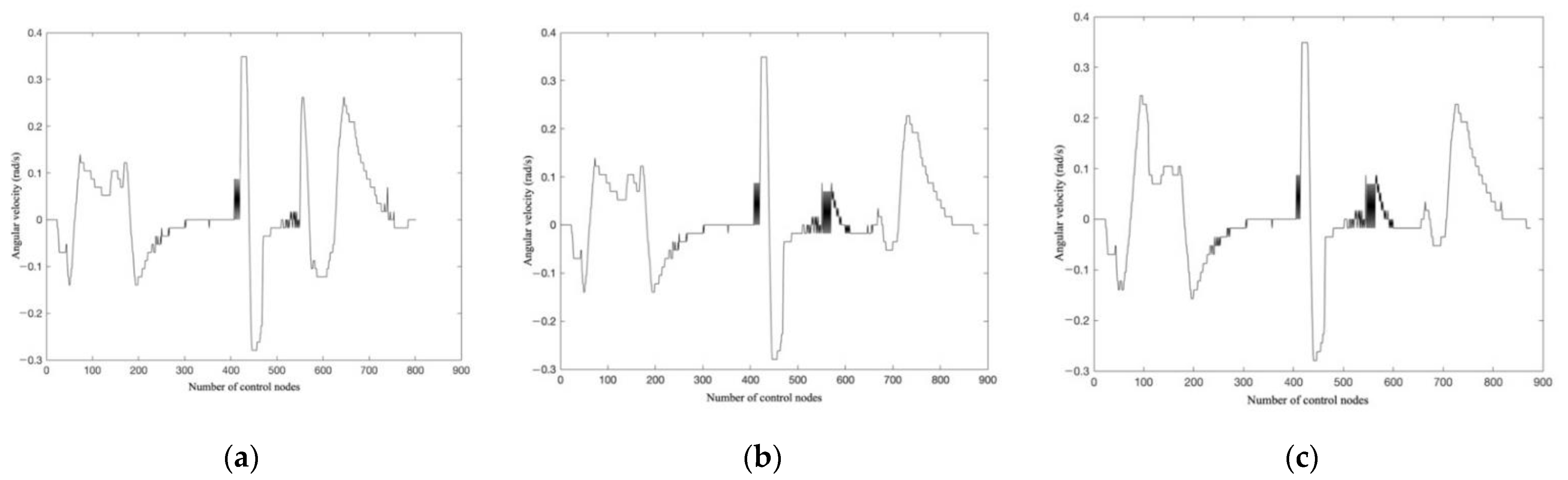
We set up three groups of simulation experiments to enhance the A* algorithm fusion dynamic window method and evaluate its ability to avoid random obstacles. A raster map with the same environment is planned using the enhanced A* algorithm and dynamic window method. The beginning coordinates are S(21,7) and the ending coordinates are T(6,25). Additionally, random obstacles are added to the map (Figure 4b). The dynamic window method has the following parameter settings: the maximum velocity is 1 m/s, the maximum angular velocity is 15°/s, and the speed resolution is 0.02 m/s with an angular velocity resolution of 1°/s, and the acceleration is 0.2 m/s2 with an angular acceleration of 50°/s2. The parameters of the evaluation function are α = 0.1, β = 0.06, and γ = 0.2. The predicted time is 4.0 s. Figure 4 depicts the outcomes of the simulation. The data for path planning is shown in Table 3, and the control parameter feedback diagram is shown in Figure 5, Figure 6 and Figure 7.
Figure 4 illustrates that when there are no random obstacles in the local diagram, the enhanced A* algorithm fusion dynamic window method plans the path from the starting point to the destination. After introducing a random obstacle, the improved A* algorithm fusion dynamic window method is able to achieve random obstacle avoidance while completing the overall path planning, and the path is smooth, preserving the globally optimal path. As can be seen in Figure 4c,d, the number of random obstacles is escalating. The path should become longer as the number of random obstacles increases, but the path between these two random obstacles is shorter than that of a random obstacle because the path planned by the dynamic window method maintains a distance from the obstacles when there is no obstacle present. Therefore, the locations of random obstacles will be added to Figure 4c so that the robot can only plan its path in close proximity to them. In conclusion, the hybrid algorithm is capable of random obstacle avoidance, and its smooth path is consistent with the globally optimal path. In contrast, the robot dynamics control requires the robot to have information regarding the continuous change in the path curvature. From Figure 5, Figure 6 and Figure 7 of the simulation results of the robot control parameters fed back by the fusion algorithm, it can be seen that the path drawn out by this fusion algorithm fully meets the requirements of the robot dynamics control.
5. Conclusions
Navigation planning a navigation path is the foundation for realizing robot navigation tracking control. Considering the robotic environment's complexity, domestic and international scholars have conducted extensive research on navigation path planning to reduce operational costs and design a better barrier-free operation path for automatic navigation in the pre-operation area. Global path planning is a mature technology widely implemented in precision operations, agricultural transportation, and machine farming across a plot schedule. Due to the complexity and spatial and temporal variability of the robotic operating environment, real-time algorithmic efficiency, robustness, and security are crucial for local path planning.
In this paper, a robot stochastic barrier avoidance method is presented that combines the improved A* algorithm and the dynamic window method. This method effectively solves the problem that the traditional A* algorithm is inefficient, has redundant nodes, and cannot randomly avoid obstacles in a complex environment. This algorithm increases the search efficiency of the A* algorithm by optimizing the A* algorithm's search point selection strategy and evaluation function. The proposed redundant node deletion strategy reduces the path length. Utilizing the dynamic window method for local planning between neighboring nodes enables the robot to avoid obstacles randomly. The following are the experimental outcomes:
First, in this paper, the path length and computation time are decreased in comparison to the traditional A* algorithm, which increases the A* algorithm's programming efficiency. There are fewer turning points and a shorter planning path in comparison to the improved A* algorithm with a 5 × 5 neighborhood and the improved A* algorithm based on hop-point search.
Second, the enhanced A* algorithm fused dynamic window method can circumvent random obstructions to reach the target point without difficulty. Based on the global path, it can correct the local path.
This research can be applied to the path planning of mobile robots in complex environments, which has some practical value. Future researchers can continue to optimize the dynamic window method's weights to enhance its environmental adaptability.
Author Contributions
Conceptualization, Y.S. and X.Z.; software, Y.S.; validation, Y.S., X.Z. and Y.Y.; investigation, Y.Y.; data curation, Y.S. and X.Z.; writing—original draft preparation, Y.S.; writing—review and editing, Y.S. and X.Z.; visualization, Y.S. and Y.Y.; supervision, X.Z.; project administration, Y.Y. All authors have read and agreed to the published version of the manuscript.
Funding
This research received no external funding.
Institutional Review Board Statement
Not applicable.
Informed Consent Statement
Not applicable.
Conflicts of Interest
The authors declare no conflict of interest.
References
- Zhang, Y.; Zhou, L. Improvement and Application of Heuristic Search in Multi-Robot Path Planning. In Proceedings of the 2017 First International Conference on Electronics Instrumentation and Information Systems, Harbin, China, 3–5 June 2017. [Google Scholar]
- Wang, H.; Li, Q.; Cheng, N. Real-Time Path Planning for Low Altitude Flight Based on A* Algorithm and TF/TA Algorithm. In Proceedings of the 2012 IEEE International Conference on Automation Science and Engineering, Seoul, Korea, 20–24 August 2012. [Google Scholar]
- Chen, R.; Xie, Y.; Yu, Y.; Zhao, H.; Lu, X.; Lu, X. Optimal path planning for obstacle avoidance of unmanned distribution vehicles based on improved A* algorithm. J. Guangdong Polytech. Norm. Univ. 2020, 41, 1–8. [Google Scholar]
- Ma, Q.; Zhang, Y.; Gong, J. Traversal path planning of agricultural robot based on memory simulated annealing and A* algorithm. J. South China Agric. Univ. 2020, 41, 127–132. [Google Scholar]
- Liu, J.; Feng, S.; Ren, J. Directed D* algorithm for dynamic path planning of mobile robots. Zhejiang Univ. J. Eng. Sci. 2020, 54, 291–300. [Google Scholar]
- Yang, X.; Cao, W.; Zhang, Y.; Fang, G.; Yan, X. Mobile Robot Path Planning in Complex Environment. In Proceedings of the 2019 IEEE International Conference on Unmanned Systems, Beijing, China, 17–19 October 2019. [Google Scholar]
- Vagale, A.; Oucheikh, R.; Bye, R.T.; Osen, O.L.; Fossen, T.I. Path planning and collision avoidance for autonomous surface vehicles I: A review. J. Mar. Sci. Technol. 2021, 26, 1292–1306. [Google Scholar] [CrossRef]
- Muthugala, M.A.V.J.; Samarakoon, S.M.B.P.; Elara, M.R. Toward energy-efficient online Complete Coverage Path Planning of a ship hull maintenance robot based on Glasius Bio-inspired Neural Network. Expert Syst. Appl. 2022, 187, 115940. [Google Scholar] [CrossRef]
- Huang, R.; Qin, C.; Li, J.L.; Lan, X. Path planning of mobile robot in unknown dynamic continuous environment using reward-modified deep Q-network. Optim. Control. Appl. Methods 2021, 1–18. [Google Scholar] [CrossRef]
- Wan, Y.; Zhong, Y.; Ma, A.; Zhang, L. An accurate UAV 3-D path planning method for disaster emergency response based on an improved multiobjective swarm intelligence algorithm. IEEE Trans. Cybern. 2022, 1–14. [Google Scholar] [CrossRef]
- Wang, Y.; Wang, L.; Chen, G.; Cai, Z.; Zhou, Y.; Xing, L. An improved ant colony optimization algorithm to the periodic vehicle routing problem with time window and service choice. Swarm Evol. Comput. 2020, 55, 100675. [Google Scholar] [CrossRef]
- Miao, C.; Chen, G.; Yan, C.; Wu, Y. Path planning optimization of indoor mobile robot based on adaptive ant colony algorithm. Comput. Ind. Eng. 2021, 156, 107230. [Google Scholar] [CrossRef]
- Sandamurthy, K.; Ramanujam, K. A hybrid weed optimized coverage path planning technique for autonomous harvesting in cashew orchards. Inf. Process. Agric. 2020, 7, 152–164. [Google Scholar] [CrossRef]
- Huang, X.; Zhang, L.; Tang, L.; Tang, C.; Li, X.; He, X. Path planning for autonomous operation of drone in fields with complex boundaries. Trans. Chin. Soc. Agric. Mach. 2020, 51, 34–42. [Google Scholar] [CrossRef]
- Zhang, D.; Zhang, Y.; Zhang, C. Data mining approach for automatic ship-route design for coastal seas using AIS trajectory clustering analysis. Ocean Eng. 2021, 236, 109535. [Google Scholar] [CrossRef]
- Xie, W.; Fang, X.; Wu, S. 2.5 D Navigation Graph and Improved A-Star Algorithm for Path Planning in Ship Inside Virtual Environment. In Proceedings of the 2020 Prognostics and Health Management Conference (PHM-Besançon), Besancon, France, 4–7 May 2020; pp. 295–299. [Google Scholar]
- Lan, X.; Lv, X.; Liu, W.; He, Y.; Zhang, X. Research on Robot Global Path Planning Based on Improved A-Star Ant Colony Algorithm. In Proceedings of the 2021 IEEE 5th Advanced Information Technology, Electronic and Automation Control Conference (IAEAC), Chongqing, China, 12–14 March 2021; pp. 613–617. [Google Scholar]
- Li, M.; Zhang, H. AUV 3D Path Planning Based on A* Algorithm. In Proceedings of the 2020 Chinese Automation Congress (CAC), Shanghai, China, 6–8 November 2020; pp. 11–16. [Google Scholar]
- Wang, J.; Chen, Z. A Novel Hybrid Map Based Global Path Planning Method. In Proceedings of the 2018 3rd Asia-Pacific Conference on Intelligent Robot Systems (ACIRS), Singapore, 21–23 July 2018; pp. 66–70. [Google Scholar]
- Liu, S.; Ma, Y.; Meng, S.; Sun, S. Improved A* algorithm for path planning of AGV. J. Comp. Appl. 2019, 39, 41–44. [Google Scholar]
- Wang, Z. Automatic robot path planning under complicit dynamic environment. Modul. Mach. Tool Autom. Manufact. Tech. 2018, 1, 64–68. [Google Scholar]
- Li, F.; Fan, X.; Hou, Z. A firefly algorithm with self-adaptive population size for global path planning of mobile robot. IEEE Access 2020, 8, 168951–168964. [Google Scholar] [CrossRef]
- Xie, Y.; Li, S.; Ying, W. A fourth-order Cartesian grid method for multiple acoustic scattering on closely packed obstacles. J. Comput. Appl. Math. 2022, 406, 113885. [Google Scholar] [CrossRef]
- Jin, Q.; Tang, C.; Cai, W. Research on dynamic path planning based on the fusion algorithm of improved ant colony optimization and rolling window method. IEEE Access 2021, 10, 28322–28332. [Google Scholar] [CrossRef]
- Chen, C.; Jiang, J.; Lv, N.; Li, S. An intelligent path planning scheme of autonomous vehicles platoon using deep reinforcement learning on network edge. IEEE Access 2020, 8, 99059–99069. [Google Scholar] [CrossRef]
- Van den Berg, J.; Lin, M.; Manocha, D. Reciprocal Velocity Obstacles for Real-Time Multi-Agent Navigation. In Proceedings of the 2008 IEEE International Conference on Robotics and Automation, Pasadena, CA, USA, 19–23 May 2008; pp. 1928–1935. [Google Scholar]
- Xu, T.; Zhang, S.; Jiang, Z.; Liu, Z.; Cheng, H. Collision avoidance of high-speed obstacles for mobile robots via maximum-speed aware velocity obstacle method. IEEE Access 2020, 8, 138493–138507. [Google Scholar] [CrossRef]
- Howard, T.M.; Kelly, A. Optimal rough terrain trajectory generation for wheeled mobile robots. Int. J. Rob. Res. 2007, 26, 141–166. [Google Scholar] [CrossRef]
- Howard, T.M.; Green, C.J.; Kelly, A.; Ferguson, D. State space sampling of feasible motions for high-performance mobile robot navigation in complex environments. J. Field Rob. 2008, 25, 325–345. [Google Scholar] [CrossRef]
- Liu, Z.; Liu, H.; Lu, Z.; Zeng, Q. A dynamic fusion pathfinding algorithm using delaunay triangulation and improved a-star for mobile robots. IEEE Access 2021, 9, 20602–20621. [Google Scholar] [CrossRef]
- Ballesteros, J.; Urdiales, C.; Velasco, A.B.M.; Ramos-Jiménez, G. A biomimetical dynamic window approach to navigation for collaborative control. IEEE Trans. Hum. Mach. Syst. 2017, 47, 1123–1133. [Google Scholar] [CrossRef]
- Hernandez, E.; Carreras, M.; Ridao, P. A comparison of homotopic path planning algorithms for robotic applications. Robot. Autonom. Syst. 2015, 64, 44–58. [Google Scholar] [CrossRef]
- Zhang, H.; Dou, L.; Fang, H.; Chen, J. Autonomous Indoor Exploration of Mobile Robots Based on Door-Guidance and Improved Dynamic Window Approach. In Proceedings of the 2009 IEEE International Conference on Robotics and Biomimetics, Guilin, China, 19–23 December 2009. [Google Scholar]
- Dobrevski, M.; Skočaj, D. Adaptive Dynamic Window Approach for Local Navigation. In Proceedings of the 2020 IEEE/RSJ International Conference on Intelligent Robots and Systems (IROS), Las Vegas, NV, USA, 24 October 2020–24 January 2021; pp. 6930–6936. [Google Scholar]
- Liu, L.; Yao, J.; He, D.; Chen, J.; Huang, J.; Xu, H.; Wang, B.; Guo, J. Global dynamic path planning fusion algorithm combining jump-A* algorithm and dynamic window approach. IEEE Access 2021, 9, 19632–19638. [Google Scholar] [CrossRef]
- Fox, D.; Burgard, W.; Thrun, S. The dynamic window approach to collision avoidance. IEEE Rob. Autom. Mag. 1997, 4, 23–33. [Google Scholar] [CrossRef]
- Li, X.; Fei, L.; Juan, L.; Liang, S. Obstacle avoidance for mobile robot based on improved dynamic window approach. Turkish J. Electr. Eng. Comput. Sci. 2017, 25, 666–676. [Google Scholar] [CrossRef]
- Vista, F.P.; Singh, A.M.; Lee, D.J.; Chong, K.T. Design convergent Dynamic Window Approach for quadrotor navigation. Int. J. Precis. Eng. Manufact. 2014, 15, 2177–2184. [Google Scholar] [CrossRef]
- Cheng, C.; Hao, X.; Li, J.; Zhang, Z.; Sun, G. Global dynamic path planning based on fusion of improved A* algorithm and dynamic window approach. J. Xi’an Jiaotong Univ. 2017, 51, 137–143. [Google Scholar] [CrossRef]
- Fan, W.; Tiejun, L.; Jinyue, L.; Haiwen, Z. Research on autonomous path planning and obstacle avoidance of building robot based on BIM. Comput. Eng. Appl. 2020, 56, 224–230. [Google Scholar] [CrossRef]
- Li, B.; Chiong, R.; Gong, L. Search-Evasion Path Planning for Submarines using the Artificial Bee Colony Algorithm. In Proceedings of the 2014 IEEE Congress on Evolutionary Computation (CEC), Beijing, China, 6–11 July 2014; pp. 528–535. [Google Scholar]
- Xu, W.; Hu, J.; Yin, J.; Li, K. Ship Automatic Collision Avoidance by Altering Course Based on Ship Dynamic Domain. In Proceedings of the 2016 IEEE Trustcom/BigDataSE/ISPA, Tianjin, China, 23–26 August 2016; pp. 2024–2030. [Google Scholar]
- Xuan, R. Research on Intelligent path Planning Based on Improved A* Algorithm and Artificial Potential Field Method. Master Thesis, Xi’an University of Electronics and Technology, Xi’an, China, 2019. [Google Scholar]
- Cheng, Y.; Xiao, H. Mobile robot dynamic path planning based on improved A* algorithm and morphin algorithm. CAAI Trans. Intell. Syst. 2020, 15, 546–552. [Google Scholar]
- Cao, Y.; Zhou, Y.; Zhang, Y.B. Path planning for obstacle avoidance of mobile robot based on optimized A* and DWA algorithm. Mach. Tool Hydraul. 2020, 48, 246–252. [Google Scholar] [CrossRef]
- Wang, Z.; Zeng, G.; Huang, B.; Fang, Z. Global optimal path planning for robots with improved A* algorithm. J. Comput. Appl. 2019, 39, 2517–2522. [Google Scholar] [CrossRef]
- Yu, W.; Zhang, Z.; Fu, X.; Wang, Z. Path planning based on map partition preprocessing and improved A* algorithm. Chin. High Technol. Lett. 2020, 30, 383–390. [Google Scholar]
- Zhang, Y.; Song, J.; Zhang, J. Local path planning of outdoor cleaning robot based on improved dynamic window method. Robot 2020, 41, 617–625. [Google Scholar] [CrossRef]
- Wang, H.; Yin, P.; Zheng, W.; Wang, H.; Zuo, J. Mobile robot path planning based on improved A* algorithm and dynamic window method. Robot 2020, 42, 346–353. [Google Scholar] [CrossRef]
- Lao, C.; Li, P.; Feng, Y. Path planning of greenhouse robot based on fusion of improved A* algorithm and dynamic window approach. Trans. Chin. Soc. Agric. Mach. 2021, 52, 14–22. [Google Scholar] [CrossRef]
Figure 1.
Schematic diagram of node moving direction.

Figure 2.
Flow of the Robot’s Random Obstacle Avoidance Algorithm Based on an Improved A* Algorithm.
Figure 2.
Flow of the Robot’s Random Obstacle Avoidance Algorithm Based on an Improved A* Algorithm.

Figure 3.
Path Planning Trajectories of Four Algorithms: (a) Path planning of four algorithms in environment I; (b) Path planning of four algorithms in environment II; (c) Path planning of four algorithms in environment III.
Figure 3.
Path Planning Trajectories of Four Algorithms: (a) Path planning of four algorithms in environment I; (b) Path planning of four algorithms in environment II; (c) Path planning of four algorithms in environment III.

Figure 4.
Path planning trajectory diagram of random obstacle avoidance: (a) Path planning without random obstacles; (b) Path planning when adding one random obstacle; (c) Path planning when adding two random obstacles; (d) Path planning when adding three random obstacles.
Figure 4.
Path planning trajectory diagram of random obstacle avoidance: (a) Path planning without random obstacles; (b) Path planning when adding one random obstacle; (c) Path planning when adding two random obstacles; (d) Path planning when adding three random obstacles.

Figure 5.
Simulation of robot attitude: (a) Path planning when adding one random obstacle; (b) Path planning when adding two random obstacles; (c) Path planning when adding three random obstacles.
Figure 5.
Simulation of robot attitude: (a) Path planning when adding one random obstacle; (b) Path planning when adding two random obstacles; (c) Path planning when adding three random obstacles.

Figure 6.
Simulation of changes in the line velocity of robots: (a) Path planning when adding one random obstacle; (b) Path planning when adding two random obstacles; (c) Path planning when adding three random obstacles.
Figure 6.
Simulation of changes in the line velocity of robots: (a) Path planning when adding one random obstacle; (b) Path planning when adding two random obstacles; (c) Path planning when adding three random obstacles.

Figure 7.
Simulation of changes in the angular velocity of robots: (a) Path planning when adding one random obstacle; (b) Path planning when adding two random obstacles; (c) Path planning when adding three random obstacles.
Figure 7.
Simulation of changes in the angular velocity of robots: (a) Path planning when adding one random obstacle; (b) Path planning when adding two random obstacles; (c) Path planning when adding three random obstacles.


Table 1.
The corresponding relationship table includes dangle and three discarding directions.
| α | Reserved Five Directions | Abandoned Three Directions |
|---|---|---|
| [337.5°, 360°) ∪ [0°, 22.5°) | n1 n2 n3 n4 n5 | n6 n7 n8 |
| [22.5°, 67.5°) | n1 n2 n3 n5 n8 | n4 n6 n7 |
| [67.5°, 112.5°) | n2 n3 n5 n7 n8 | n1 n4 n6 |
| [112.5°, 157.5°) | n3 n5 n6 n7 n8 | n1 n2 n4 |
| [157.5°, 202.5°) | n4 n5 n6 n7 n8 | n1 n2 n3 |
| [202.5°, 247.5°) | n1 n4 n6 n7 n8 | n2 n3 n5 |
| [247.5°, 292.5°) | n1 n2 n4 n6 n7 | n3 n5 n8 |
| [292.5°, 337.5°) | n1 n2 n3 n4 n6 | n5 n7 n8 |
Table 2.
Path Regularization Results of 4 Algorithms.
| Algorithms | Environment I | Environment II | Environment III | ||||||
|---|---|---|---|---|---|---|---|---|---|
| after Smoothing Length /m | Time/s | Number of Turning Points | after Smoothing Length /m | Time/s | Number of Turning Points | after Smoothing Length /m | Time/s | Number of Turning Points | |
| Traditional A* Algorithm | 33.1891 | 0.0075562 | 15 | 31.2136 | 0.01507 | 24 | 20.0765 | 0.004029 | 18 |
| An Improved A* Algorithm for a 5 × 5 Neighborhood Search | 33.2204 | 0.017705 | 14 | 32.1737 | 0.02704 | 19 | 20.0739 | 0.011244 | 15 |
| An Improved A* Algorithm for Path Planning | 33.1737 | 0.035745 | 8 | 31.7024 | 0.044917 | 12 | 20.1634 | 0.019895 | 12 |
| An Improved A* Algorithm Based on Hop Search | 32.6157 | 0.055889 | 10 | 31.7562 | 0.062665 | 13 | 19.7577 | 0.029458 | 13 |
Table 3.
Path planning performance of improved A* algorithm fusing dynamic window method.
| Number of Random Obstacles | Path Length/m | Time/s |
| One random obstacle | 28.9960 | 112.3578 |
| Two random obstacle | 28.9770 | 121.7401 |
| Three random obstacle | 29.3370 | 122.9477 |
Publisher’s Note: MDPI stays neutral with regard to jurisdictional claims in published maps and institutional affiliations. |
© 2022 by the authors. Licensee MDPI, Basel, Switzerland. This article is an open access article distributed under the terms and conditions of the Creative Commons Attribution (CC BY) license (https://creativecommons.org/licenses/by/4.0/).
Share and Cite
MDPI and ACS Style
Sun, Y.; Zhao, X.; Yu, Y. Research on a Random Route-Planning Method Based on the Fusion of the A* Algorithm and Dynamic Window Method. Electronics 2022, 11, 2683. https://doi.org/10.3390/electronics11172683
AMA Style
Sun Y, Zhao X, Yu Y. Research on a Random Route-Planning Method Based on the Fusion of the A* Algorithm and Dynamic Window Method. Electronics. 2022; 11(17):2683. https://doi.org/10.3390/electronics11172683
Chicago/Turabian StyleSun, Yicheng, Xianliang Zhao, and Yazhou Yu. 2022. "Research on a Random Route-Planning Method Based on the Fusion of the A* Algorithm and Dynamic Window Method" Electronics 11, no. 17: 2683. https://doi.org/10.3390/electronics11172683
Note that from the first issue of 2016, this journal uses article numbers instead of page numbers. See further details here.