Deep Learning Spatial-Spectral Classification of Remote Sensing Images by Applying Morphology-Based Differential Extinction Profile (DEP)

Abstract

Since the technology of remote sensing has been improved recently, the spatial resolution of satellite images is getting finer. This enables us to precisely analyze the small complex objects in a scene through remote sensing images. Thus, the need to develop new, efficient algorithms like spatial-spectral classification methods is growing. One of the most successful approaches is based on extinction profile (EP), which can extract contextual information from remote sensing data. Moreover, deep learning classifiers have drawn attention in the remote sensing community in the past few years. Recent progress has shown the effectiveness of deep learning at solving different problems, particularly segmentation tasks. This paper proposes a novel approach based on a new concept, which is differential extinction profile (DEP). DEP makes it possible to have an input feature vector with both spectral and spatial information. The input vector is then fed into a proposed straightforward deep-learning-based classifier to produce a thematic map. The approach is carried out on two different urban datasets from Pleiades and World-View 2 satellites. In order to prove the capabilities of the suggested approach, we compare the final results to the results of other classification strategies with different input vectors and various types of common classifiers, such as support vector machine (SVM) and random forests (RF). It can be concluded that the proposed approach is significantly improved in terms of three kinds of criteria, which are overall accuracy, Kappa coefficient, and total disagreement.

1. Introduction

With the increased spatial resolution of recently produced imaging sensors, a considerable amount of remote sensing satellite images, especially very high-resolution (VHR) images, are available. These images provide us with more information in greater detail about the land surface. The fine spatial optical sensors with metric or sub metric resolution, such as QuickBird, GeoEye, Pleiades, and World-View, allow detecting fine-scale objects, such as residential housing elements, commercial buildings, and transportation systems and utilities. However, the large-scale nature of these datasets introduces new challenges in image analysis.

Many applications, such as land resource management, urban planning, precise agriculture, and crisis management [1,2,3,4,5,6], rely on very high-resolution remote sensing imagery. One of the most crucial tasks for accurate information extraction from these images is classification, which classifies the scene’s objects into meaningful categories. Unfortunately, these categories are almost identical to each other in many cases, such as pastureland and agricultural farmland or trees and grass. So, we have difficulty distinguishing similar types, especially in a complex scene with many details. Accordingly, it is crucial to find a proper classification method that enables us to address this issue.

It is now proven that spatial information integration can improve accuracy, particularly with VHR images [7]. The spatial information can determine the shape and size of the objects in the image, which is very helpful to reduce the noisy appearance of classified pixels in the final result. This happens a lot when the classifier uses only spectral information without considering spatial arrangements.

There are two common strategies to extract spatial information from VHR images: the crisp neighbourhood system [8,9,10] and the adaptive neighbourhood system [11,12,13]. The former considers a predefined neighbourhood system with a static shape, while the latter is based on modifying the neighbourhood system.

Markov random field (MRF)-based approaches and artificial neural networks (ANN) are examples of the first group [9,10,13,14]. Although these methodologies can lead to an increase in final accuracy, they suffer from some shortcomings. For example, a predefined neighbourhood system cannot characterize the specifications of objects with different sizes. The smaller items may disappear in the final map, or the larger ones may turn into pieces.

The other family of methods are based on sparse representation (SR) [15,16]. These methods are primarily pixel-wise sparse models but they usually incorporate the spatial context to the joint sparse model (JSM) [17,18,19]. Using multiple-scale regions for each pixel and shaping a multiscale SR model is proposed in [20] to contain complementary spatial information. However, optimal integration of spatial information is still a big challenge in this area of study.

To address the above issues, methodologies based on adaptive neighbourhood system are suggested, such as segmentation-based [21,22], morphological profiles (MPs) [23,24], attribute profiles (APs) [13,25], and extinction profiles (EPs) [26,27]. These approaches have their own limitations too. For example, segmentation algorithms extract image objects and generate relevant results according to specific criteria. Image objects in a scene, especially in urban areas, generally show multiscale or multilevel features. Therefore, they appear at different scales of analysis. So, the procedure for choosing the best scale is very complicated and time-consuming [21].

The other contributions that use adaptive neighbourhood systems are based on morphological profiles (MPs). MPs are usually composed of applying opening or closing by reconstructions with a structuring element (SE) of different sizes. The introduction of the MP concept leads to creating the morphological spectrum for each pixel [28,29,30,31,32]. Another study in this area is based on the derivative of MP introduced in [33], which has more promising results. However, as an SE’s shape is fixed, different objects with different shapes cannot be accurately modelled. Besides, MPs are unable to extract information related to grey-level specifications of the objects in the image.

One can use the morphological attribute profile (AP) instead of morphological profile to address the shortcomings mentioned above. The concept of AP has been introduced first in [25] to generalize MPs. This new concept uses sequential morphological attribute filters (AFs). So, it can provide a multilevel characterization of the image.

APs work based on connectivity rules. Thus, they only consider connected components in the image. Compared to the MPs, APs are more flexible because they can view different attributes to model the image’s structural information. Several studies are based on the APs, which can be found in [25,34] for classification and building extraction tasks. If multiple attributes have been taken into account, an extended AP (EAP) can be created.

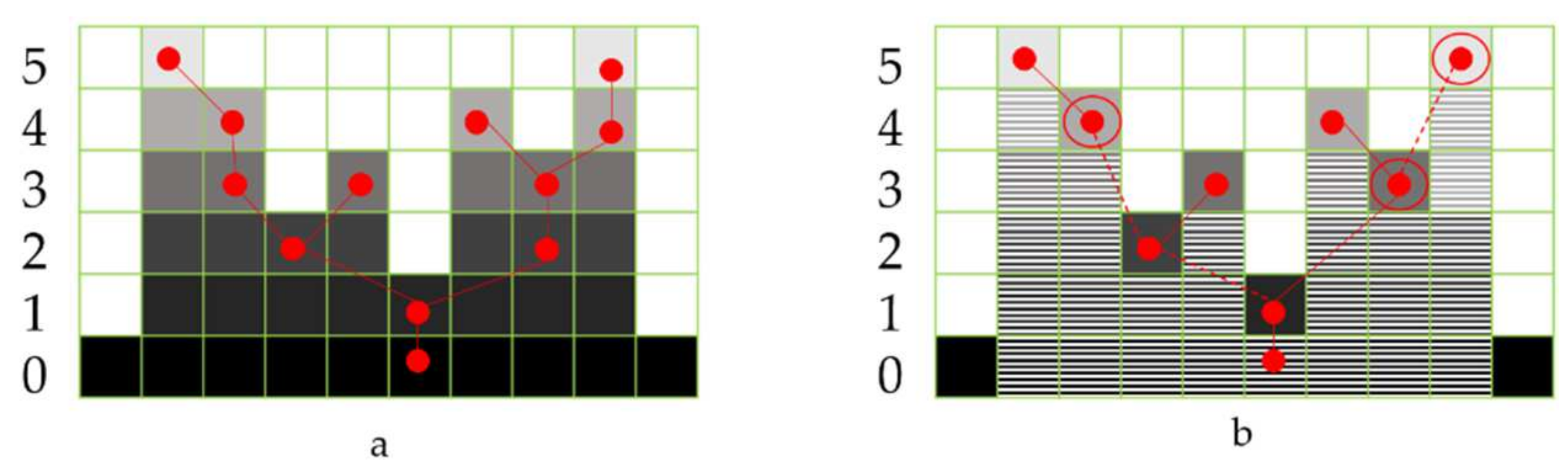
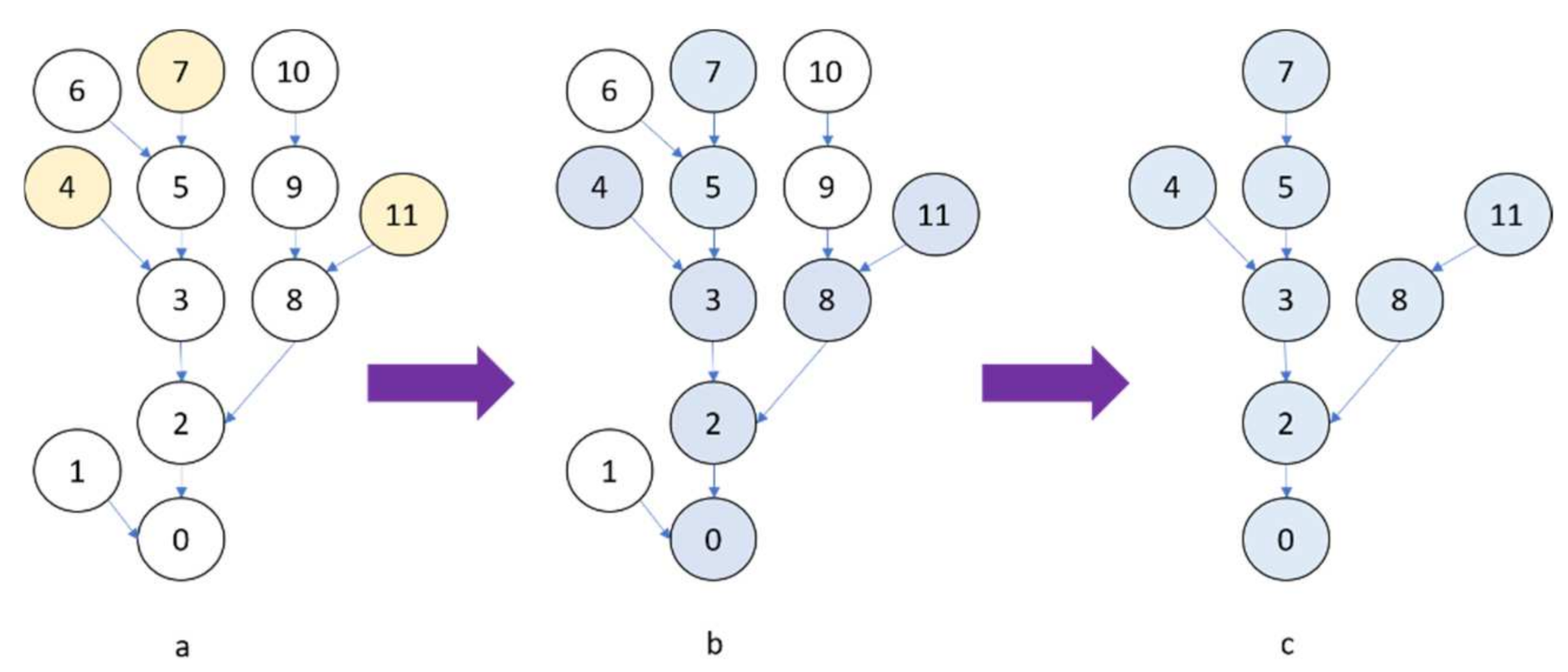
The other different variant of MPs, known as extinction profiles (EPs), is introduced in [7], and they have shown promising results. EP’s implementation is based on the tree-representation (max-tree) [35]. This concept will be thoroughly discussed in the next section.

The EP can create features for every pixel in the image with contextual information. Different methodologies have been tested to classify these features efficiently. Various studies, such as [13,36,37], have been undertaken in this area. They mostly use support vector machine (SVM), random forest (RF), or artificial neural networks (ANNs) for spatial-spectral classification purposes, but they all have some limitations. For example, advanced SVMs with kernels like Gaussian or radial basis functions (RBFs) can handle the imbalance of the size of the image and the number of training samples. However, kernel SVMs cause overfitting in the case of sparse feature space [38]. They also require several parameters to be set.

Random forest is another option for classification purposes that has been vastly used in different studies [38,39,40,41]. Although random forest-based methods are fast and yield stable results, their performance is easily influenced by the size of training samples [42].

Another classification method that has been used more recently in the remote sensing community is artificial neural networks. ANNs are biologically inspired and multilayer classes of deep learning models that use a single neural network trained end to end from input vector obtained from image to classifier outputs [43]. However, the standard ANNs are limited when dealing with multidimensional images because they need to adjust many parameters for neurons in the layer to reach satisfactory accuracy [44]. Lately, deep networks have been demonstrated to achieve significant empirical improvements in most of the remote sensing fields like spatial-spectral classification [22,45,46,47,48]. Many spatial-based techniques including semantic segmentation continuously advance. They have been employed to address remote sensing problems that are diverse and data-rich in nature [49]. Examples of these researches include environmental monitoring [50], crop cover and analysis [51,52], types of trees in forests [53], and building detection [54]. Deep learning methods automatically extract features that are tailored for the classification tasks, which makes such methods better choices for handling complicated approaches [55]. The unique structure of the deep learning network may be able to learn features in different layers and adjust the parameters, at running time, based on accuracy, giving more importance to one layer than another depending on the problem [47]. As the deep networks show great robustness and effectiveness in image classification, they have the potential to cope with the difficulties of non-linear spatial-spectral image analysis.

In this paper, a robust, precise approach is proposed to automatically extract spatial-spectral information from VHR images and classify them into thematic classes. In more detail, the main contributions of the paper are listed below:

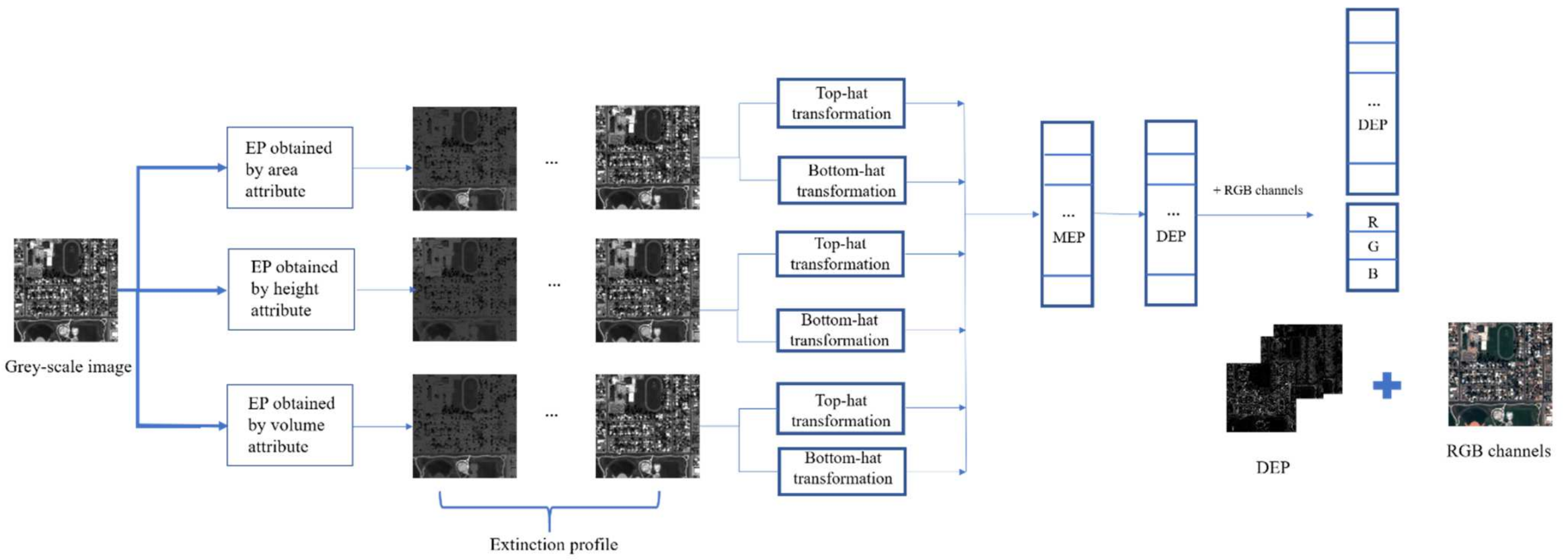
• The paper applies a morphological spectrum, including differential extinction profile (DEF) and spectral information, to address the pixel specifications for further classification.
• The differential extinction profile (DEF) used in the study is processed using morphology-based filters such as top-hat and bottom-hat filters. This leads to producing a concise, informative feature vector.
• As the extinction profile automatically used a different number of extrema to make a complete profile, there is no need to set any parameters in the proposed approach. So, it can be used for different datasets with different characteristics.
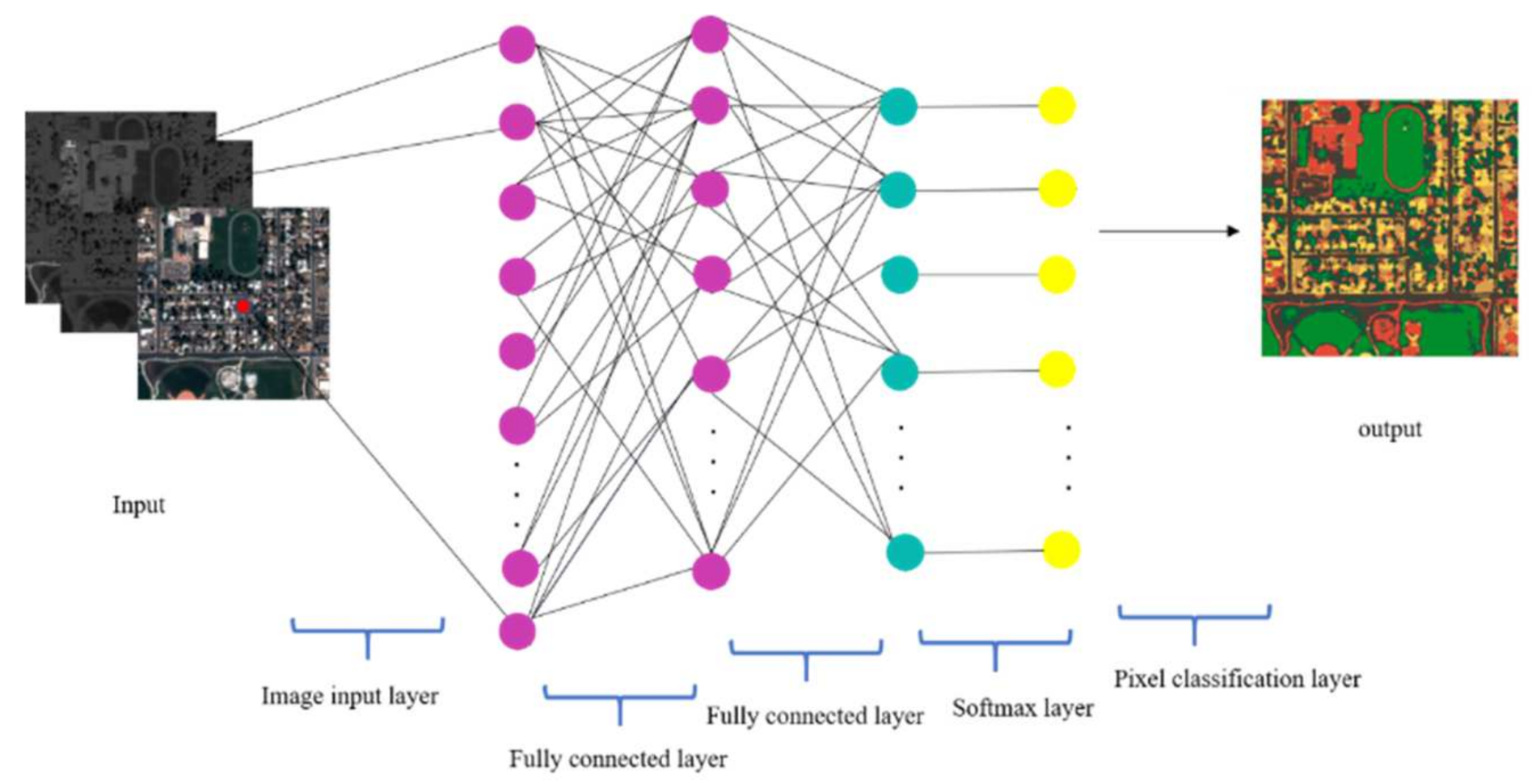
• A simple, straightforward, yet accurate deep learning-based neural network has been developed for classification purposes.
• The proposed approach is applied to different datasets. The entire process is fully automatic and speedy.

The remainder of this paper is organized as follows. The mathematical foundations of EP and deep-learning-based classifiers are addressed in the Section 2. The proposed approach is explained in detail in the Section 3. The experimental analyses, evaluations, and comparisons are presented in Section 4, and the last section is attributed to the conclusion.

2. Mathematical Background

The concept of morphological profile (MP) was introduced in [23]. It has been widely applied as a powerful approach to extract contextual information from the image by modelling structural features (e.g., size, geometry etc.). In this section, we first explain the so-called tree representation of the image (max-tree), which is essential for the implementation of the extinction profile (EP), a very recent variant of MPs. Then, we discuss EPs and their equations. The last part is dedicated to deep learning classification.

2.1. Max-Tree

Max-tree is a data structure representing a grey-scale image as a tree based on the hierarchical property of threshold decomposition [56]. It was first introduced in [57] to implement connected filters.

Informally speaking, if we have a grey-scale image, a specific threshold leads to a binary image, where each white island (with value 1) is a connected component. The higher the threshold value, the smaller the size of connected components. The component tree shows the hierarchical relationship of its connected components which are obtained through threshold decomposition, and the max-tree is a compact representation of this component tree. The max-tree nodes store only the pixels that are visible at a specific threshold (or grey level). Therefore, the connected components that remain unchanged for a sequence of thresholds are represented in a single node, called composite node [35,58].

There are four major steps in the max-tree algorithm: (1) tree creation usually using maxima, (2) marking the nodes that do not meet the criteria, (3) filtering the nodes, and (4) image recovery [25]. The underlying concept of max-tree has been displayed in Figure 1. Imagine a 1-D image with gray levels: f = {0, 5, 4, 2, 3, 1, 4, 3, 5, 0} [56]. The double circles are max-tree composite nodes, and the leaves of both component tree and max-tree are related to regional maxima. Efficient implementations of extinction filters, and thus extinction profiles, are needed to take advantage of the max-tree concept.

2.2. Extinction Profile

Extinction filters (EF) are connected filters that preserve the leaf node or the extrema of the image related to the connected component of the image. The connected filters are idempotent, i.e., they do not blur the image and only make alternations to the image the first time they applied [56,59]. If extinction filters have been implemented using max-tree structure, the number of maxima (max-tree leaves) with the highest extinction values, according to chosen attribute, are selected. All other nodes have been cut from the tree. Therefore, there are three parameters to be set in order to apply extinction filters on the image: the kind of extrema chosen to be filtered (usually the maxima of the image), the attribute filter, and the number of extrema to be kept. Imagine that $Max(X)=\{M_1,M_2,\dots ,M_N\}$ shows the regional maxima’s set in the image $X$, and $N$ represents the number of regional maxima. $M_i(i=1,\dots ,N)$ is the obtained image of the same size of $X$, with zero in all other positions except for the pixels that compose the regional maxima. Each $M_i$ has the extinction value according to the selected attribute. The extinction of $X$ set to keep the $n$ extrema that has the highest extinction values is given by [60]:

$$E{F}^n(X)=R_X^{\delta }(G)$$

(1)

where $R_X^{\delta }(G)$ is the reconstruction by dilation [61] of the mask image $X$ from the marker image $G$. The marker $G$ image can be obtained by:

$$G=\underset{i=1}{\overset{n}{Max\left\{M_i^{\prime }\right\}}}$$

(2)

where $Max$ is the pixel-wise maximum operation for the regional maxima related to the extinction value, $M_1^{\prime }$ is the regional maxima with the highest extinction value, $M_2^{\prime }$ has the second-highest extinction value, and so on. Figure 2 displays the EF concept visually.

Extinction profile (EP) can produce a precise analysis of the input image. EPs are a series of thinning and thickening transformations, i.e., EFs, applied on a grey-scale image with progressively higher threshold values. In this manner, spatial and contextual information can be extracted from image comprehensively. If $T_{w^{{\mu }_k}}$ and $T_{b^{{\mu }_k}}$ denote the thinning and thickening morphological transformations, EPs can be described as a concatenation of them, as given by:

$$EP(X)=\left\{\begin{array}{l}{T}_{w^{{\mu }_k}},k=(s-i+1),\forall i\in [1,s];\\ T_{b^{{\mu }_k}},k=(i-s),\forall i\in [s+1,2s]\end{array}\right\}$$

(3)

where ${\mu }_k$ is the criteria or threshold that will change in each iteration and s is the number of them. The set of ordered $\mu$ is ${\mu }_i,{\mu }_j\in \mu \mathrm{and}j\ge i$ $\mu =\{{\mu }_1,{\mu }_2,\dots {\mu }_s\}$. For ${\mu }_i,{\mu }_j\in \mu \mathrm{and}j\ge i$, the relation ${\mu }_i\le {\mu }_j$ holds for thickening and ${\mu }_i\ge {\mu }_j$ holds for thinning. The total number of images produced by EP will be (2s + 1), including the original grey-scale image.

EPs can be obtained using different types of attributes like area, volume, or height with a different number of extrema values. The higher number of values preserve more details, while a smaller number produces smoother results. The more the number of extrema decreases, the more unnecessary information is omitted. Please note that, for the EP, the feature produced by the higher number of extrema is placed closer to the input image in the profile. The hierarchical relationship between the images generated by the EP is $T_{w^{{\mu }_1}}\ge T_{w^{{\mu }_2}}\ge \dots \ge T_{w^{{\mu }_s}}\ge T_{b^{{\mu }_s}}\ge T_{b^{{\mu }_s-1}}\ge \dots \ge T_{b^{{\mu }_1}}$.

Unlike MPs that can only model the size and the structure of objects in the scene, EPs are flexible and have different types. Thus, multiples EPs (MEP) can be created by concatenating various kinds of EPs (i.e., area height and volume).

$$MEP=\left\{E{P}_{area},E{P}_{voulme},E{P}_{height}\right\}$$

(4)

Since MEP considers different types of attributes, it can extract more contextual information than a single EP.

2.3. Deep Learning for Classification

Deep learning or, strictly speaking, deep neural network (DNN), refers to a kind of neural network with two or more hidden layers aside from the input and output layer [56]. Like other neural networks, DNNs consist of neurons that implement mathematical functions with trainable parameters.

A typical DNN learns hierarchical image features by stacking different types of layers. The neuron including linear or nonlinear transformations is formulated as follows [62]:

$$a=f(WX+b)$$

(5)

where $a$ is the activation function of the neuron, $X$ is the input vector, W is the weight vector, $b$ is the bias term, and $f$ is the nonlinear activation function. Typically, an activation function can be a logistic sigmoid function $sigmoid(x)=1/1+e^{-x}$ or rectified linear units (ReLU) $ReLU(x)=max(0,x)$ [63]. Neural networks with at least one nonlinear activation function can represent any complex function [64]. For classification purposes, one neural network can take an image as an input and output class scores. The label of each pixel can be obtained with the class scores [65]. The goal of training is to find optimal parameters (i.e., vector weights) to predict the right labels. The loss function (i.e., cost function) aims to evaluate the performance of the system by comparing predicted class scores and the corresponding ground truth. In this study, we used the cross-entropy loss function to evaluate the performance of the neural network, which is defined as follows

$$L_{score}=-log(\frac{e^{f_j}}{{\displaystyle \sum _i{e}^{f_i}}})$$

(6)

where $f_i$ is the ith class score and $f_j$ is the score related to the ground truth label. In most cases, a regularization loss is added by penalizing a large number of parameters using $L_2$ regularization. Then, the total loss is defined as follows:

$$L=L_{score}+\lambda {\displaystyle \sum _i{W}_i^2}$$

(7)

where $W_i$ means the ith element in weight vector and $\lambda$ is a parameter which controls the importance of regularization loss. Using the regularization loss, the loss function will be strictly convex with a unique solution.

The process of network training is an optimization problem that aims at minimizing the loss function. Usually, the gradient descent methods are used for this purpose. There are two steps in the process of optimizing: (1) computation of the gradient of the loss function with respect to the weight vectors; (2) updating the parameters following the gradient. The parameters can be obtained as follows for one iteration:

$$W_i=W_{i-1}-lr\times \frac{\partial L}{\partial W_{i-1}}$$

(8)

where $W_i$ is the ith element of the weight vector, $lr$ is the learning rate, and $\partial L/\partial W_{i-1}$ is the derivative of parameters. The gradient is calculated by backpropagation which recursively computes the derivative of parameters according to the chain rule.

3. Deep-Learning-Based Approach for Spatial-Spectral Classification

3.1. The Framework of the Proposed Approach

The first step in the proposed approach is to extract contextual information. A practical concept based on EP that can enrich the input feature vector of classification is differential extinction profile (DEP), which is the difference between two subsequent images in MEP. In fact, instead of using the original pixel value of each MEP image, the derivative of them will be applied. The number of DEP feature vectors is one less than MEP and can be computed by [7]:

$$DEP(X)=\left\{\begin{array}{l}{\Delta }_{T_{w_k}(X)},k=(s-i+1),\forall i\in [1,s]\\ {\Delta }_{T_{b_k}(X)},k=(s-n),\forall i\in [n+1,2s]\end{array}\right\}$$

(9)

where ${\Delta }_{T_{w_k}(X)}$ and ${\Delta }_{T_{b_k}(X)}$ are the derivatives of thickening and thinning profile, respectively. Here, in this study, top-hat and bot-hat transformations were applied to produce a thickening and thinning profile. The attributes used for the computation of DEP are area, height, and volume.

After the computation of DEP, the spectral information, which is the information of RGB channels, is added to the contextual information. The final feature vector is created to be fed to the deep-learning-based network. Figure 3 is a thematic display of the proposed approach.

The deep network designed for the classification is straightforward. Inspired by [66], it constitutes an input layer, which, in this case, has 14 channels. The next two layers are fully connected layers. A fully connected layer is a layer in which the neurons connect to all the neurons in the next layer. The second fully connected layer combines the feature obtained by the first one to classify the image. Then, a softmax classification layer is used. The softmax activation function normalized the output of the previous layer. The outcome of this layer can be interpreted as classification probabilities by the final layer. The last layer is the classification layer that assigns each input to the mutually exclusive classes and computes the loss. The architecture of the proposed DNN is displayed in Figure 4. The final thematic map result is the output of this network.

3.2. Algorithm Setup

The number of maxima used in this study to compute DEP for each attribute is 10, which are $s=\{1,2,4,8,16,32,64,128,256,512\}$. All profiles were calculated using the 4-connectivity condition. DEP was calculated using the derivative of three consecutive images in the MEP vector instead of two sequential images to have a compressive input vector. The whole process’s implementation was done through the “siamxt” python toolbox [67] using Google Colab.

To have a fair comparison, first, the input feature vector was introduced into two different classification methods, namely SVM and RF. The SVM classifier has a one-versus-one coding design with L1QP solver. The random forest classifier has 50 trees.

Second, in addition to the input feature vector produced using the mentioned procedure in the previous section. The differential morphological profile (DMP) was applied. The DMP concept was used for different applications, such as image segmentation and classification [61,68]. Analogous to the DEP-based feature vector, the DMP-based feature vector was classified using SVM and RF besides deep learning. We test all classification methods using only spectral information (RGB) too. This part of the proposed approach was done through Matlab 2020a. The experiments were run on a system with two 2.3 GHz eight-core CPUs and 16 GB memory.

For DNN implementation, we use the stochastic gradient descent with momentum (SDGM) solver, with momentum 0.8 and gradient threshold 10. The size of the mini-batch to use for each training iteration is 128. We also shuffle the training data before each training epoch and shuffle the validation data before each network validation.

Eventually, the final classification map was modified using a 5 × 5 median filter to remove salt-and-pepper noise from the classification result.

4. Experimental Analysis

4.1. Data Description

Two VHR images were selected to illustrate the proposed approach’s operation: a Pleiades dataset and a World-View 2 dataset.

The first dataset was acquired by Pleiades image. It is a subset of a pan-sharpened product from Pleiades image over Commerce City, CO, USA. The dimension of this data is 999 × 999 and the spatial resolution is about 0.5 m. The ground reference for this image is obtained by manual photo interpretation. The reference data contain six different classes of interest: trees, grass, asphalt, soil, roof type 1 and 2. The number of test and train pixels selected for the classification step is tabulated in

Table 1. The number of test and train pixels of Pleiades image.

Name of the Class	No. Test	No. Train
Trees	94,827	2292
Grass	9124	832
Road	34,743	1242
Soil	10,478	574
Roof type 1	2957	344
Roof type 2	6339	520

. The original image, ground reference, and index of classes are displayed in Figure 5.

The second dataset was captured of the city of Riyadh, Saudi Arabia, by World-View 2. The size of the image is 1080 × 1920 at spatial resolution of 0.46 m. Similar to the Pleiades dataset, the ground reference of eight different classes was distinguished manually: Trees, grass, asphalt, roof type 1, 2, and 3, soil, and shadow. The roof classes were separated into three different types since they have different colours. The number of test and train pixels selected for the classification step has been tabulated in

Table 2. The number of test and train pixels of World-View 2 image.

Name of the Class	No. Test	No. Train
Trees	46,580	4952
Grass	6937	782
Asphalt	7874	1302
Roof type 1	3542	651
Roof type 2	8490	1032
Roof type 3	11,025	1664
Soil	11,130	2144
Shadow	7178	1506

. The original image, ground reference, and index of them are displayed in Figure 6.

4.2. Results and Discussion

In this study, three different classifiers have been used, i.e., SVM, RF, and newly proposed DNN, which were implemented using three different input vectors. Two of them have both spatial and spectral information (DEP and DMP). The third one has only spectral information (RGB).

The classification accuracies are evaluated through four measures, namely overall accuracy (OA), kappa coefficient (K), f-score (F), and total disagreement (T). the first three ones were applied widely in remote sensing applications. The last one is the sum of two new criteria named quantity and allocation disagreements introduced in [49]. It is claimed that they can provide a more precise accuracy assessment for RS images than Kappa families. Since the Kappa indices may be useless, misleading, or flawed for practical applications in remote sensing, it is recommended that instead of using the Kappa coefficient, the professionals summarize the confusion matrix with two more specific summary parameters of quantity and allocation disagreements. The allocation disagreement is described as the amount of difference between the reference map and a comparison map, which is less than an optimal match in the spatial allocation of the categories, with respect to the available classes in the reference and comparison maps. The quantity disagreement is defined as the amount of difference between the reference map and a comparison map that is less than a perfect match regarding the available categories in the reference and comparison maps. The sum of these two measures is called total disagreement (T). T is calculated for two experimental datasets.

Table 3. Kappa coefficient for Pleiades dataset.

	DEP + RGB	DMP + RGB	RGB
Deep learning	0.87928	0.7709	0.7386
SVM	0.83090	0.7945	0.7806
RF	0.82647	0.8206	0.7928

,

Table 4. Overall accuracy for Pleiades dataset.

	DEP + RGB	DMP + RGB	RGB
Deep learning	93.0505	86.2551	84.5200
SVM	89.9259	87.3406	86.3814
RF	89.4630	88.9565	87.2837

and

Table 5. Total disagreement for Pleiades dataset.

	DEP + RGB	DMP + RGB	RGB
Deep learning	0.0694	0.1374	0.1548
SVM	0.1007	0.1265	0.1361
RF	0.1053	0.1104	0.1271

represent classification accuracy measures (K, OA and T) for the Pleiades dataset. The OA for a deep-learning-based classifier with DEP + RGB input vector is about 93%, which is at least 3% better than the following best method.

As can be seen, the proposed approach outperforms other methods’ results in terms of all criteria.

DEP + RGB can produce a more accurate result regardless of the classifier type in terms of total disagreement. The overall accuracy and Kappa coefficient for DEP + RGB column confirm this fact. On the other hand, each table’s last row shows that only spectral information is not enough if high accuracy is intended. Looking at the second column, we find that the input vector constructed with DEP’s help in all cases has a better result than the input vector constructed with the help of DMP. This is due to the fact that DEP can consider different types of attributes and preserve regions suitable for distinguishing classes.

As observed in Figure 7, only the DNN classifier with DEP + RGB input vector successfully distinguishes the correct class around the sports field, soil and not the asphalt or roof. In fact, a deep learning strategy was able to make the most of spatial-spectral information to connect the training samples to their correspondence classes. The asphalt and soil are visually similar, and an amateur interpreter may make a mistake recognizing these classes. So, it is not enough to have an informative input feature vector, and it is crucial to choose a robust classifier.

Considering the information in

Table 6. The f-score measure for all classes in the Pleiades dataset.

	Trees	Grass	Asphalt	Roof Type 1	Roof Type 2	Soil
Deep learning with DEP + RGB	0.9719	0.5189	0.9443	0.9390	0.7691	0.7882
Deep learning with DMP + RGB	0.9244	0.2598	0.9191	0.9591	0.0112	0.7027
Deep learning with RGB	0.9429	0.3494	0.8789	0.9619	0.4099	0.7251
SVM with DEP + RGB	0.9559	0.5176	0.9313	0.9116	0.6664	0.6837
SVM with DMP + RGB	0.9315	0.4626	0.9325	0.9925	0.6307	0.5587
SVM with RGB	0.9150	0.4455	0.9454	0.9808	0.6009	0.5325
RF with DEP + RGB	0.9457	0.5381	0.9345	0.9078	0.7173	0.6910
RF with DMP + RGB	0.9421	0.5248	0.9197	0.9768	0.7262	0.7505
RF with RGB	0.9310	0.4475	0.9249	0.9806	0.6890	0.7141

proves that the proposed approach outperforms all other methods for three classes: trees, roof type 2, and soil. For class asphalt, the SVM method with RGB is slightly better. The difference between the two numbers is 0.0011. For class roof type 1, the SVM classifier with DMP + RGB has a more accurate result (about 0.05). However, it does not have an accurate f-score for classes grass, soil, and roof type 2. Likewise, the RF classifier with DEP + RGB has the best result for class grass. However, its performance for soil and roof type 2 is poor. Thus, they cannot be considered outstanding classifiers.

Table 7. Kappa coefficient for World-View 2 dataset.

	DEP + RGB	DMP + RGB	RGB
Deep learning	0.8594	0.8291	0.80311
SVM	0.8026	0.8415	0.8258
RF	0.8135	0.8242	0.7204

,

Table 8. Overall accuracy for World-View 2 dataset.

	DEP + RGB	DMP + RGB	RGB
Deep learning	89.5052	87.3379	85.4023
SVM	85.5959	87.9646	87.5285
RF	85.7156	86.6645	77.6898

and

Table 9. Total disagreement for World-View 2 dataset.

	DEP + RGB	DMP + RGB	RGB
Deep learning	0.1049	0.1266	0.1459
SVM	0.1440	0.1203	0.1218
RF	0.1428	0.1333	0.2231

provide information about the classification accuracy attained by different strategies for the second dataset here, World-View 2. Like the Pleiades case, the proposed approach outperforms the other methods. In this manner, the overall accuracy is about 2%, and total disagreement is about 0.02 better than the best results of other different strategies. Moreover, the classifiers fed with only spectral information show the least accurate results, expectedly.

Table 10. The f-score measure for all classes in World-View 2 dataset.

	Trees	Grass	Asphalt	Roof Type 1	Roof Type 2	Roof Type 3	Soil	Shadow
Deep learning with DEP + RGB	0.9490	0.6968	0.9619	0.8493	0.9368	0.9403	0.7701	0.7433
Deep learning with DMP + RGB	0.9507	0.8176	0.7804	0.6537	0.7610	0.8693	0.9116	0.7086
Deep learning with RGB	0.9303	0.7163	0.9878	0.9409	0.8835	0.3900	0.6995	0.6783
SVM with DEP + RGB	0.9175	0.6243	0.9999	0.9085	0.5622	0.7971	0.9137	0.6659
SVM with DMP + RGB	0.9562	0.8501	0.9979	0.4911	0.9086	0.5692	0.9674	0.8420
SVM with RGB	0.9237	0.6275	0.9997	0.5711	0.9134	0.6483	0.9497	0.7633
RF with DEP + RGB	0.8922	0.6365	0.9999	0.8729	0.7923	0.8463	0.8536	0.8431
RF with DMP + RGB	0.9396	0.8688	0.9977	0.8235	0.7191	0.6677	0.8723	0.7503
RF with RGB	0.8064	0.5358	0.9999	0.5457	0.8990	0.6935	0.8593	0.7496

shows the f-score measure for the World-View2 dataset. The proposed approach’s superiority can be found when considering the roof classes type 1, 2, and 3. Although these three classes are similar to each other, the deep learning classifier with DEP + RGB input vector can have promising outcomes: about 84, 94, and 94 in terms of f-score. The other strategies may have a precise result for one of the classes, but they perform poorly in distinguishing the other ones. For example, SVM with the DMP + RGB method distinguishes the grass class successfully, but it performs poorly in distinguishing class roof types 1 and 3. It can be said that inadequate training samples can reduce accuracy when the image classes are made up of small, similar objects. For this reason, a classifier that can extract all classes with high accuracy is of particular importance. With its spatial information, the proposed approach compensates for the lack of training data and allocates spatial-spectral information to the correct class with DNN. Figure 8 displays all thematic maps yielded from different classifiers.

Finally, considering all the classes in the image, the proposed method is superior to the competing methods.

5. Conclusions

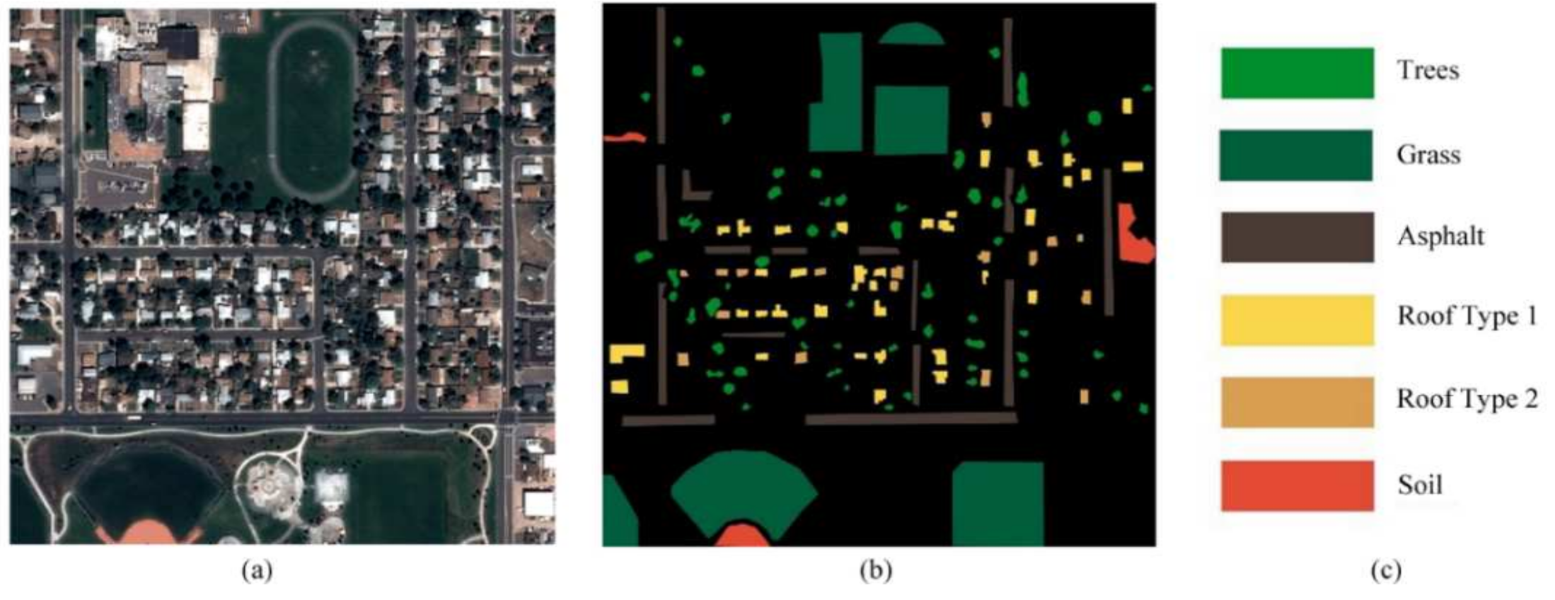
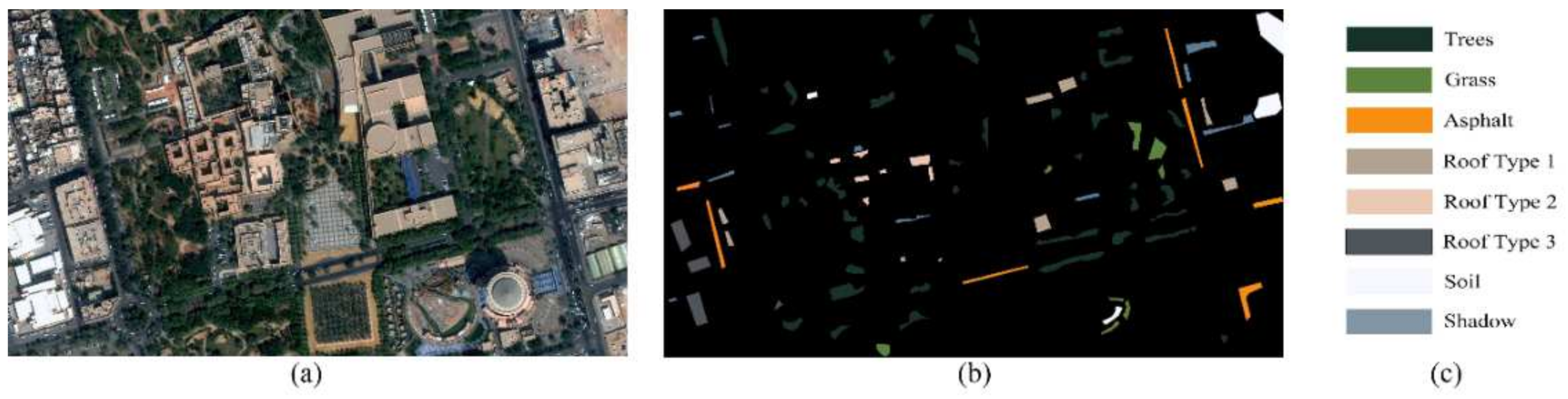
This paper proposes a novel approach for the spatial-spectral classification of very high-resolution remote sensing data. The proposed approach is based on the differential extinction profile (DEP) concept. The DEP is the derivative of extinction profile (EP) that can be made by applying top-hat and bottom-hat transformation on a grey-scale image. The DEP extracts geometrical information from an image with different kinds of attributes such as area, height, and volume. The spectral information, which is the RGB channels, have been added to DEP to build an input feature vector. This vector is incorporated in a straightforward deep learning classifier that does not contain complicated architecture with so many parameters.

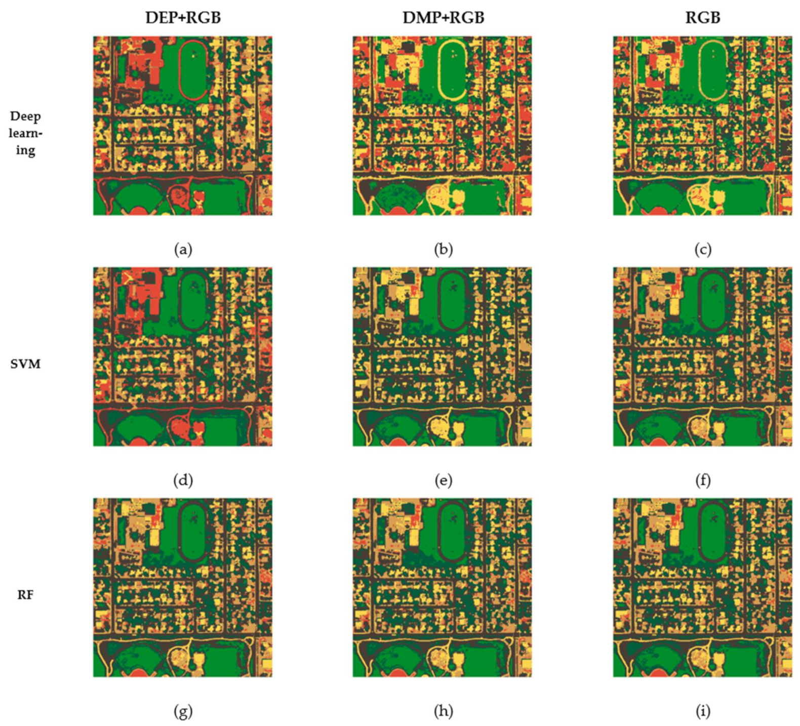
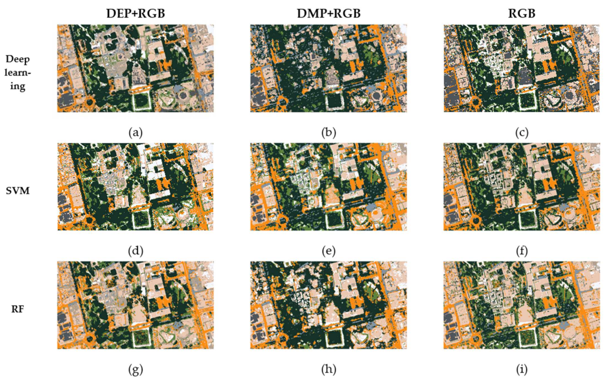
The proposed approach has been performed on two VHR datasets: the Pleiades and the World-View 2 urban images. The obtained results have been compared with two of the most robust methods in the literature, i.e., support vector machine (SVM) and random forest (RF). We have also tested all mentioned classifiers through different types of the input vector, which are DMP + RGB and only RGB bands. To have a fair comparison, four types of criteria have been applied in this study, which are: overall accuracy (OA), Kappa coefficient (K), f-score (F), and total disagreement (T).

With respect to the experiments, it can be concluded that the newly proposed approach yields a more accurate final classification map than other methods. All four measures verified this claim. According to this research, the following points can be noted: (1) DEPs are capable of extracting contextual information so they can improve the classification accuracies due to their ability to preserve more correspondences in the image. (2) Our method includes different types of image attributes, like area, height, and volume, so it provides more promising results than other types of morphological profiles like MPs. (3) Incorporating spatial and spectral information in a robust, straightforward deep neural network makes the whole approach easy-to-use and implement. (4) The proposed approach is fully automatic and there is no need to set additional parameters.

In the future, it will be helpful to add an edge detection algorithm to the proposed approach to exclude edge pixels from the classification process. In this way, the final thematic map will be finer for practical use.

References

1. Rohith, G.; Kumar, L.S. Paradigm shifts in super-resolution techniques for remote sensing applications. Vis. Comput. 2021, 37, 1965–2008. [Google Scholar] [CrossRef]
2. Wang, B.; Lu, X.; Zheng, X.; Li, X. Semantic Descriptions of High-Resolution Remote Sensing Images. IEEE Geosci. Remote Sens. Lett. 2019, 16, 1274–1278. [Google Scholar] [CrossRef]
3. Li, Z.; Shen, H.; Cheng, Q.; Liu, Y.; You, S.; He, Z. Deep learning based cloud detection for medium and high resolution remote sensing images of different sensors. ISPRS J. Photogramm. Remote Sens. 2019, 150, 197–212. [Google Scholar] [CrossRef] [Green Version]
4. Zhang, C.; Wei, S.; Ji, S.; Lu, M. Detecting Large-Scale Urban Land Cover Changes from Very High Resolution Remote Sensing Images Using CNN-Based Classification. ISPRS Int. J. Geo-Inf. 2019, 8, 189. [Google Scholar] [CrossRef] [Green Version]
5. Gao, L.; Song, W.; Dai, J.; Chen, Y. Road Extraction from High-Resolution Remote Sensing Imagery Using Refined Deep Residual Convolutional Neural Network. Remote Sens. 2019, 11, 552. [Google Scholar] [CrossRef] [Green Version]
6. Li, Y.; Xu, L.; Rao, J.; Guo, L.; Yan, Z.; Jin, S. A Y-Net deep learning method for road segmentation using high-resolution visible remote sensing images. Remote Sens. Lett. 2019, 10, 381–390. [Google Scholar] [CrossRef]
7. Ghamisi, P.; Souza, R.; Benediktsson, J.A.; Zhu, X.X.; Rittner, L.; Lotufo, R. Extinction Profiles for the Classification of Remote Sensing Data. IEEE Trans. Geosci. Remote Sens. 2016, 54, 5631–5645. [Google Scholar] [CrossRef]
8. Ghamisi, P.; Benediktsson, J.A.; Ulfarsson, M.O. Spectral–Spatial Classification of Hyperspectral Images Based on Hidden Markov Random Fields. IEEE Trans. Geosci. Remote Sens. 2013, 52, 2565–2574. [Google Scholar] [CrossRef] [Green Version]
9. Chen, Y.; Jiang, H.; Li, C.; Jia, X.; Ghamisi, P. Deep Feature Extraction and Classification of Hyperspectral Images Based on Convolutional Neural Networks. IEEE Trans. Geosci. Remote Sens. 2016, 54, 6232–6251. [Google Scholar] [CrossRef] [Green Version]
10. Moser, G.; Serpico, S.B.; Benediktsson, J.A. Land-Cover Mapping by Markov Modeling of Spatial–Contextual Information in Very-High-Resolution Remote Sensing Images. Proc. IEEE 2012, 101, 631–651. [Google Scholar] [CrossRef]
11. Acquarelli, J.; Marchiori, E.; Buydens, L.M.; Tran, T.; Van Laarhoven, T. Spectral-Spatial Classification of Hyperspectral Images: Three Tricks and a New Learning Setting. Remote Sens. 2018, 10, 1156. [Google Scholar] [CrossRef] [Green Version]
12. Benediktsson, J.A.; Ghamisi, P. Spectral-Spatial Classification of Hyperspectral Remote Sensing Images; Artech House: London, UK, 2015. [Google Scholar]
13. Ghamisi, P.; Mura, M.D.; Benediktsson, J.A. A Survey on Spectral–Spatial Classification Techniques Based on Attribute Profiles. IEEE Trans. Geosci. Remote Sens. 2014, 53, 2335–2353. [Google Scholar] [CrossRef]
14. Zhong, Y.; Lin, X.; Zhang, L. A Support Vector Conditional Random Fields Classifier With a Mahalanobis Distance Boundary Constraint for High Spatial Resolution Remote Sensing Imagery. IEEE J. Sel. Top. Appl. Earth Obs. Remote Sens. 2014, 7, 1314–1330. [Google Scholar] [CrossRef]
15. Chen, Y.; Nasrabadi, N.M.; Tran, T.D. Hyperspectral Image Classification via Kernel Sparse Representation. IEEE Trans. Geosci. Remote Sens. 2012, 51, 217–231. [Google Scholar] [CrossRef] [Green Version]
16. Srinivas, U.; Chen, Y.; Monga, V.; Nasrabadi, N.M.; Tran, T.D. Exploiting Sparsity in Hyperspectral Image Classification via Graphical Models. IEEE Geosci. Remote Sens. Lett. 2012, 10, 505–509. [Google Scholar] [CrossRef] [Green Version]
17. Fu, W.; Li, S.; Fang, L.; Kang, X.; Benediktsson, J.A. Hyperspectral Image Classification Via Shape-Adaptive Joint Sparse Representation. IEEE J. Sel. Top. Appl. Earth Obs. Remote Sens. 2016, 9, 556–567. [Google Scholar] [CrossRef]
18. Fang, L.; Wang, C.; Li, S.; Benediktsson, J.A. Hyperspectral Image Classification via Multiple-Feature-Based Adaptive Sparse Representation. IEEE Trans. Instrum. Meas. 2017, 66, 1646–1657. [Google Scholar] [CrossRef]
19. Li, J.; Zhang, H.; Zhang, L. Efficient Superpixel-Level Multitask Joint Sparse Representation for Hyperspectral Image Classification. IEEE Trans. Geosci. Remote Sens. 2015, 53, 5338–5351. [Google Scholar] [CrossRef]
20. Fang, L.; Li, S.; Kang, X.; Benediktsson, J.A. Spectral–Spatial Hyperspectral Image Classification via Multiscale Adaptive Sparse Representation. IEEE Trans. Geosci. Remote Sens. 2014, 52, 7738–7749. [Google Scholar] [CrossRef]
21. Kakhani, N.; Mokhtarzade, M.; Zouj, M.J.V. Classification of very high-resolution remote sensing images by applying a new edge-based marker-controlled watershed segmentation method. Signal Image Video Process. 2019, 13, 1319–1327. [Google Scholar] [CrossRef]
22. Zhao, H.; Qi, X.; Shen, X.; Shi, J.; Jia, J. ICNet for Real-Time Semantic Segmentation on High-Resolution Images. In Proceedings of the Transactions on Petri Nets and Other Models of Concurrency XV; Springer Science and Business Media LLC: Berlin, Germany, 2018; pp. 418–434. [Google Scholar]
23. Pesaresi, M.; Benediktsson, J.A. A new approach for the morphological segmentation of high-resolution satellite imagery. IEEE Trans. Geosci. Remote Sens. 2001, 39, 309–320. [Google Scholar] [CrossRef] [Green Version]
24. Fauvel, M.; Chanussot, J.; Benediktsson, J.A.; Sveinsson, J.R. Spectral and spatial classification of hyperspectral data using SVMs and morphological profiles. IEEE Trans. Geosci. Remote Sens. 2007, 46, 4834–4837. [Google Scholar] [CrossRef] [Green Version]
25. Mura, M.D.; Benediktsson, J.A.; Waske, B.; Bruzzone, L. Morphological Attribute Profiles for the Analysis of Very High Resolution Images. IEEE Trans. Geosci. Remote Sens. 2010, 48, 3747–3762. [Google Scholar] [CrossRef]
26. Fang, L.; He, N.; Li, S.; Ghamisi, P.; Benediktsson, J.A. Extinction Profiles Fusion for Hyperspectral Images Classification. IEEE Trans. Geosci. Remote Sens. 2017, 56, 1803–1815. [Google Scholar] [CrossRef]
27. Ghamisi, P.; Hofle, B.; Zhu, X.X. Hyperspectral and LiDAR Data Fusion Using Extinction Profiles and Deep Convolutional Neural Network. IEEE J. Sel. Top. Appl. Earth Obs. Remote Sens. 2016, 10, 3011–3024. [Google Scholar] [CrossRef]
28. Tamminga, A.D.; Hugenholtz, C.H.; Eaton, B.C.; Lapointe, M. Hyperspatial Remote Sensing of Channel Reach Morphology and Hydraulic Fish Habitat Using an Unmanned Aerial Vehicle (UAV): A First Assessment in the Context of River Research and Management. River Res. Appl. 2015, 31, 379–391. [Google Scholar] [CrossRef]
29. Kaur, B.; Garg, A. Mathematical morphological edge detection for remote sensing images. In Proceedings of the 2011 3rd International Conference on Electronics Computer Technology, Kanyakumari, India, 8–10 April 2011; Volume 5, pp. 324–327. [Google Scholar]
30. Soille, P.; Pesaresi, M. Advances in mathematical morphology applied to geoscience and remote sensing. IEEE Trans. Geosci. Remote Sens. 2002, 40, 2042–2055. [Google Scholar] [CrossRef]
31. Benediktsson, J.A.; Pesaresi, M.; Arnason, K. Classification and feature extraction for remote sensing images from urban areas based on morphological transformations. IEEE Trans. Geosci. Remote Sens. 2003, 41, 1940–1949. [Google Scholar] [CrossRef] [Green Version]
32. Valero, S.; Chanussot, J.; Benediktsson, J.; Talbot, H.; Waske, B. Advanced directional mathematical morphology for the detection of the road network in very high resolution remote sensing images. Pattern Recognit. Lett. 2010, 31, 1120–1127. [Google Scholar] [CrossRef] [Green Version]
33. Chanussot, J.; Benediktsson, J.A.; Fauvel, M. Classification of Remote Sensing Images From Urban Areas Using a Fuzzy Possibilistic Model. IEEE Geosci. Remote Sens. Lett. 2006, 3, 40–44. [Google Scholar] [CrossRef] [Green Version]
34. Mura, M.D.; Benediktsson, J.A.; Waske, B.; Bruzzone, L. Modeling structural information for building extraction with morphological attribute filters. In Image and Signal Processing for Remote Sensing XV; International Society for Optics and Photonics: Bellingham, WA, USA, 2009; p. 747703. [Google Scholar]
35. Souza, R.; Tavares, L.; Rittner, L.; Lotufo, R. An Overview of Max-Tree Principles, Algorithms and Applications. In Proceedings of the 2016 29th SIBGRAPI Conference on Graphics, Patterns and Images Tutorials (SIBGRAPI-T), Sao Paulo, Brazil, 4–7 October 2016; pp. 15–23. [Google Scholar]
36. Huang, X.; Guan, X.; Benediktsson, J.A.; Zhang, L.; Li, J.; Plaza, A.; Mura, M.D. Multiple Morphological Profiles From Multicomponent-Base Images for Hyperspectral Image Classification. IEEE J. Sel. Top. Appl. Earth Obs. Remote Sens. 2014, 7, 4653–4669. [Google Scholar] [CrossRef]
37. Marpu, P.R.; Pedergnana, M.; Mura, M.D.; Peeters, S.; Benediktsson, J.A.; Bruzzone, L. Classification of hyperspectral data using extended attribute profiles based on supervised and unsupervised feature extraction techniques. Int. J. Image Data Fusion 2012, 3, 269–298. [Google Scholar] [CrossRef]
38. Belgiu, M.; Drăguţ, L. Random forest in remote sensing: A review of applications and future directions. ISPRS J. Photogramm. Remote Sens. 2016, 114, 24–31. [Google Scholar] [CrossRef]
39. Chutia, D.; Bhattacharyya, D.K.; Sarma, K.; Kalita, R.; Sudhakar, S. Hyperspectral Remote Sensing Classifications: A Perspective Survey. Trans. GIS 2015, 20, 463–490. [Google Scholar] [CrossRef]
40. Colditz, R.R. An Evaluation of Different Training Sample Allocation Schemes for Discrete and Continuous Land Cover Classification Using Decision Tree-Based Algorithms. Remote Sens. 2015, 7, 9655–9681. [Google Scholar] [CrossRef] [Green Version]
41. Karlson, M.; Ostwald, M.; Reese, H.; Sanou, J.; Tankoano, B.; Mattsson, E. Mapping Tree Canopy Cover and Aboveground Biomass in Sudano-Sahelian Woodlands Using Landsat 8 and Random Forest. Remote Sens. 2015, 7, 10017–10041. [Google Scholar] [CrossRef] [Green Version]
42. Du, P.; Samat, A.; Waske, B.; Liu, S.; Li, Z. Random Forest and Rotation Forest for fully polarized SAR image classification using polarimetric and spatial features. ISPRS J. Photogramm. Remote Sens. 2015, 105, 38–53. [Google Scholar] [CrossRef]
43. Hu, W.; Huang, Y.; Wei, L.; Zhang, F.; Li, H.-C. Deep Convolutional Neural Networks for Hyperspectral Image Classification. J. Sens. 2015, 2015, 1–12. [Google Scholar] [CrossRef] [Green Version]
44. Sharma, A.; Liu, X.; Yang, X.; Shi, D. A patch-based convolutional neural network for remote sensing image classification. Neural Networks 2017, 95, 19–28. [Google Scholar] [CrossRef] [PubMed]
45. Liang, J.; Xu, J.; Shen, H.; Fang, L. Land-use classification via constrained extreme learning classifier based on cascaded deep convolutional neural networks. Eur. J. Remote Sens. 2020, 53, 219–232. [Google Scholar] [CrossRef]
46. Heipke, C.; Rottensteiner, F. Deep learning for geometric and semantic tasks in photogrammetry and remote sensing. Geo-Spat. Inf. Sci. 2020, 23, 10–19. [Google Scholar] [CrossRef]
47. Nogueira, K.; Penatti, O.A.; dos Santos, J.A. Towards better exploiting convolutional neural networks for remote sensing scene classification. Pattern Recognit. 2017, 61, 539–556. [Google Scholar] [CrossRef] [Green Version]
48. Romero, A.; Gatta, C.; Camps-Valls, G. Unsupervised Deep Feature Extraction for Remote Sensing Image Classification. IEEE Trans. Geosci. Remote Sens. 2015, 54, 1349–1362. [Google Scholar] [CrossRef] [Green Version]
49. Ball, J.E.; Anderson, D.T.; Chan Sr, C.S. Comprehensive survey of deep learning in remote sensing: Theories, tools, and challenges for the community. J. Appl. Remote Sens. 2017, 11, 042609. [Google Scholar] [CrossRef] [Green Version]
50. Yuan, X.; Sarma, V. Automatic Urban Water-Body Detection and Segmentation From Sparse ALSM Data via Spatially Constrained Model-Driven Clustering. IEEE Geosci. Remote Sens. Lett. 2010, 8, 73–77. [Google Scholar] [CrossRef]
51. Yang, S.; Chen, Q.; Yuan, X.; Liu, X. Adaptive Coherency Matrix Estimation for Polarimetric SAR Imagery Based on Local Heterogeneity Coefficients. IEEE Trans. Geosci. Remote Sens. 2016, 54, 6732–6745. [Google Scholar] [CrossRef]
52. Jadhav, J.; Singh, R.P. Automatic semantic segmentation and classification of remote sensing data for agriculture. Math. Model. Eng. 2018, 4, 112–137. [Google Scholar] [CrossRef]
53. Dechesne, C.; Mallet, C.; Le Bris, A.; Gouet-Brunet, V. Semantic Segmentation of Forest Stands of Pure Species as a Global Optimization Problem. ISPRS Ann. Photogramm. Remote Sens. Spat. Inf. Sci. 2017, IV-1/W1, 141–148. [Google Scholar] [CrossRef] [Green Version]
54. Fang, F.; Yuan, X.; Wang, L.; Liu, Y.; Luo, Z. Urban Land-Use Classification From Photographs. IEEE Geosci. Remote Sens. Lett. 2018, 15, 1927–1931. [Google Scholar] [CrossRef]
55. Yuan, X.; Shi, J.; Gu, L. A review of deep learning methods for semantic segmentation of remote sensing imagery. Expert Syst. Appl. 2021, 169, 114417. [Google Scholar] [CrossRef]
56. Ghamisi, P.; Maggiori, E.; Li, S.; Souza, R.; Tarablaka, Y.; Moser, G.; De Giorgi, A.; Fang, L.; Chen, Y.; Chi, M.; et al. New Frontiers in Spectral-Spatial Hyperspectral Image Classification: The Latest Advances Based on Mathematical Morphology, Markov Random Fields, Segmentation, Sparse Representation, and Deep Learning. IEEE Geosci. Remote Sens. Mag. 2018, 6, 10–43. [Google Scholar] [CrossRef]
57. Salembier, P.; Oliveras-Vergés, A.; Garrido, L. Antiextensive connected operators for image and sequence processing. IEEE Trans. Image Process. 1998, 7, 555–570. [Google Scholar] [CrossRef] [Green Version]
58. Souza, R.; Rittner, L.; Machado, R.; Lotufo, R. Maximal Max-Tree Simplification. In Proceedings of the 2014 22nd International Conference on Pattern Recognition, Stockholm, Sweden, 24–28 August 2014; pp. 3132–3137. [Google Scholar]
59. Li, W.; Wang, Z.; Li, L.; Du, Q. Modified Extinction Profiles for Hyperspectral Image Classification. In Proceedings of the 2018 10th IAPR Workshop on Pattern Recognition in Remote Sensing (PRRS), Beijing, China, 19–20 August 2018; pp. 1–5. [Google Scholar] [CrossRef]
60. Vachier, C.; Meyer, F. Extinction value: A new measurement of persistence. In IEEE Workshop on Nonlinear Signal and Image Processing; IEEE: Halkidiki, Greece, 1995; Volume 1, pp. 254–257. [Google Scholar]
61. Soille, P. Morphological Image Analysis; Springer Science and Business Media LLC: Berlin, Germany, 2004. [Google Scholar]
62. Sun, W.; Wang, R. Fully Convolutional Networks for Semantic Segmentation of Very High Resolution Remotely Sensed Images Combined With DSM. IEEE Geosci. Remote Sens. Lett. 2018, 15, 474–478. [Google Scholar] [CrossRef]
63. Krizhevsky, A.; Sutskever, I.; Hinton, G.E. Imagenet classification with deep convolutional neural networks. Adv. Neural Inf. Process. Syst. 2012, 25, 1097–1105. [Google Scholar] [CrossRef]
64. Haykin, S.S. Neural Networks and Learning Machines/Simon Haykin; Prentice Hall: New York, NY, USA, 2009. [Google Scholar]
65. Maggiori, E.; Tarabalka, Y.; Charpiat, G.; Alliez, P. Convolutional Neural Networks for Large-Scale Remote-Sensing Image Classification. IEEE Trans. Geosci. Remote Sens. 2017, 55, 645–657. [Google Scholar] [CrossRef] [Green Version]
66. Isikdogan, L.F.; Bovik, A.; Passalacqua, P. Seeing Through the Clouds with DeepWaterMap. IEEE Geosci. Remote Sens. Lett. 2020, 17, 1662–1666. [Google Scholar] [CrossRef]
67. Souza, R.; Rittner, L.; Machado, R.; Lotufo, R. iamxt: Max-tree toolbox for image processing and analysis. SoftwareX 2017, 6, 81–84. [Google Scholar] [CrossRef]
68. Akçay, H.G.; Aksoy, S. Automatic Detection of Geospatial Objects Using Multiple Hierarchical Segmentations. IEEE Trans. Geosci. Remote Sens. 2008, 46, 2097–2111. [Google Scholar] [CrossRef]
Figure 1. (a) Component tree and (b) Max-tree of sample image f = {0, 5, 4, 2, 3, 1, 4, 3, 5, 0}. The composite nodes are depicted by double circles and the filled pixels in each horizontal connected component represent the pixels each node stores.
Electronics 10 02893 g001
Figure 2. (a) The original tree; the yellow nodes show the nodes with the highest extinction values (b) Blue nodes represent the path from the three leaf nodes with the highest extinction values to the root (c) Results of the modification of nodes is not marked in blue.
Electronics 10 02893 g002
Figure 3. The framework of computation of input feature vector.
Electronics 10 02893 g003
Figure 4. The architecture of the proposed DNN.
Electronics 10 02893 g004
Figure 5. (a) Pleiades subset (b) Ground reference (c) Index.
Electronics 10 02893 g005
Figure 6. (a) World-View 2 subset (b) Ground reference and (c) Index.
Electronics 10 02893 g006
Figure 7. The classification results of (a) Deep learning with DEP + RGB (b) Deep learning with DMP + RGB (c) Deep learning with RGB (d) SVM with DEP + RGB (e) SVM with DMP + RGB (f) SVM with RGB (g) RF with DEP + RGB (h) RF with DMP + RGB (i) RF with RGB for Pleiades dataset.
Electronics 10 02893 g007
Figure 8. The classification results of (a) Deep learning with DEP + RGB (b) Deep learning with DMP + RGB (c) Deep learning with RGB (d) SVM with DEP + RGB (e) SVM with DMP + RGB (f) SVM with RGB (g) RF with DEP + RGB (h) RF with DMP + RGB (i) RF with RGB for World-View 2 dataset.
Electronics 10 02893 g008