
CA-CRE: Classification Algorithm-Based Controller Area Network Payload Format Reverse-Engineering Method


1
Department of Computer Engineering, Ajou University, Suwon 16499, Korea
2
Department of Cyber Security, Ajou University, Suwon 16499, Korea
*
Author to whom correspondence should be addressed.
Electronics 2021, 10(19), 2442; https://doi.org/10.3390/electronics10192442
Submission received: 9 September 2021
/
Revised: 30 September 2021
/
Accepted: 4 October 2021
/
Published: 8 October 2021
(This article belongs to the Special Issue Data-Driven Security)
Abstract
:In vehicles, dozens of electronic control units are connected to one or more controller area network (CAN) buses to exchange information and send commands related to the physical system of the vehicles. Furthermore, modern vehicles are connected to the Internet via telematics control units (TCUs). This leads to an attack vector in which attackers can control vehicles remotely once they gain access to in-vehicle networks (IVNs) and can discover the formats of important messages. Although the format information is kept secret by car manufacturers, CAN is vulnerable, since payloads are transmitted in plain text. In contrast, the secrecy of message formats inhibits IVN security research by third-party researchers. It also hinders effective security tests for in-vehicle networks as performed by evaluation authorities. To mitigate this problem, a method of reverse-engineering CAN payload formats is proposed. The method utilizes classification algorithms to predict signal boundaries from CAN payloads. Several features were uniquely chosen and devised to quantify the type-specific characteristics of signals. The method is evaluated on real-world and synthetic CAN traces, and the results show that our method can predict at least 10% more signal boundaries than the existing methods.
1. Introduction
Modern vehicles are increasingly connected to the outside world through various channels, such as cellular networks, Wi-Fi, Bluetooth, and DSRC. Due to this connectivity, substantial offensive security research on vehicles [1,2,3,4,5,6] has shown that vehicles are susceptible to attacks intended to gain remote access and control. Most of the attacks aim to obtain write-access to in-vehicle networks (IVNs) and eventually send control commands to manipulate the vehicles. Thus, vehicles are required to have in-depth security that can secure not only external interfaces such as telematics control units (TCUs) but also IVNs such as the CAN bus itself.
IVNs are bus networks that support information exchange among dozens of electronic control units (ECUs). Communication protocols, such as controller area networks (CAN), CAN-FD, FlexRay, MOST, and Ethernet, are used for IVNs. Although CAN has the lowest bandwidth among these, it is widely used since it has advantages in terms of cost and robustness [7,8,9]. However, security was not considered when it was initially designed, and it has a limited maximum data size of eight bytes per frame. The characteristics of CAN make it difficult to use signature schemes such as message authentication code (MAC) and elliptic curve digital signature algorithm (ECDSA) for distinguishing between valid messages from ECUs and malicious messages from external attackers.
CAN protocol defines the data link layer and part of the physical layer [10]. In the upper layer of CAN, car manufacturers define their own proprietary protocols, which vary by car model. The format information of an upper-layer proprietary protocol is stored in a file called database for CAN (DBC), which is kept secret by car manufacturers. An attacker who wants to gain write-access to a CAN bus of a specific vehicle is required to find out this information to control the vehicle. However, securing the format information itself can be regarded as the security through obscurity paradigm [11,12]. It may add additional reverse-engineering burden to attackers, but it cannot prevent the attacks. The study of C. Miller and C. Valasek [1] demonstrated that one can discover important CAN messages (kill engine, steering, etc.) from an off-the-shelf vehicle, including how checksums are generated. Moreover, dozens of reverse-engineered DBC files already exist on the internet [13]. However, the secrecy of the message format inhibits IVN security research (e.g., intrusion detection systems) by third-party researchers.
The secrecy of format information also hinders effective security tests for in-vehicle networks as performed by third-party evaluation organizations. ISO/SAE 21434 [14] states that component cybersecurity testing for vehicles should be performed to search for unidentified vulnerabilities; this includes a penetration test, vulnerability scanning and fuzz testing. Thus, evaluation authorities such as the Korea Transport Safety Authority are required to evaluate not only the physical safety but also cyber security aspects of vehicles to be released. However, authorities cannot force car manufacturers to reveal their proprietary format information, which leads to less effective evaluation in the security of in-vehicle networks of the vehicles under test.
To mitigate the problem, a classification algorithm-based CAN reverse-engineering method (CA-CRE) is proposed in this paper to identify CAN message formats using a classifier. CA-CRE is composed mainly of two phases: the learning phase and prediction phase. In the first phase, a dataset to train a classifier is extracted from CAN traces, whose format information is already revealed. The dataset is a table, where each row represents nine feature values and a label of a signal (a field defined in DBC). The features are statistical values that can be extracted from CAN traces. They are chosen and devised to quantify the characteristics of signals. Then, the dataset is given to one of the machine-learning classification models as training data. In the second phase, prediction of signal boundaries for a CAN trace is performed. First, preliminary signal boundaries are extracted from the CAN trace. Then, the final signal boundaries are predicted within the preliminary boundaries using the classifier trained earlier.
CA-CRE and the previous works, READ [11] and LibreCAN [12], are evaluated on a real-world CAN trace and synthetic CAN traces. The synthetic traces are used to test the methods on a large amount of data, which is difficult to obtain in the real world. Based on the evaluation, the proposed method predicts 12% more boundaries than previous works on the real-world CAN trace [15]. The method also outperforms previous works on the synthetic CAN traces by predicting 15.9% more signals.
Contributions of the proposed method reside in two aspects. In terms of defensive security, the method minimizes the manual efforts required for IVN security research as studied by third-party researchers. In terms of offensive security, the proposed work increases the effectiveness of security tests on the CAN bus of an arbitrary vehicle, so that the test can be operated as a gray-box test instead of black-box test. One can perform penetration testing or fuzz testing on arbitrary vehicles and discover new vulnerabilities more effectively if more signal information is provided.
This paper is organized as follows. Section 2 describes the background and related work. Section 3 describes the proposed signal boundary reverse-engineering method. The performance measurements and a comparison of the results of the proposed method and existing studies are provided in Section 4. Section 5 includes a discussion of the proposed method. Lastly, our work is concluded in Section 6.
2. Background and Related Work
Controller Area Network is a communication protocol developed by Bosch in 1983, and it has been widely used in the automotive industry. In CANs, each node represents an ECU, an embedded device with sensors and actuators attached. The ECU reads information from its surroundings by using sensors and performs appropriate actions through actuators. The IVN of a vehicle is composed of a bus network or multiple bus networks with tens of ECUs connected to the networks. The data line of the CAN bus uses a twisted pair line consisting of CAN_H and CAN_L, and all nodes on the network are connected to the two lines so that all messages transmitted on the bus can be received. Each CAN message contains a unique identifier, which is 11 bits in the CAN standard format and 29 bits in the extended format. The identifier is also known as an arbitration ID (AID), which determines message priority. When two nodes attempt to broadcast a message to the CAN bus simultaneously, the message with the smaller ID value gains access first. A CAN message is composed of one or more signals that have their own fixed starting bit position and size. Each signal carries one type of information, such as RPM, speed of front-left wheel, counter value, and checksum. Receiving nodes only receive messages with the specific IDs they require and ignore the rest of the messages.
While the data link layer is defined in the CAN standard, upper-layer protocols are proprietary and vary by car manufacturer and model. The specifications of a vehicle’s CAN payload format information are stored in a proprietary format [16] called DBC. For each arbitration ID, size of payload, receiving nodes, and signals are defined in DBC. Descriptions of each signal, such as name, bit position, size, scale, offset, min/max, unit, and endian, are also contained in DBC.
The first attempt to reverse-engineer message formats of CAN payloads was the study of Markovitz et al. [17]. The study aimed to design a domain-aware anomaly detection system that identifies malicious packets that do not comply with the reverse-engineered format. To infer payload format, the method categorizes signals into four types (const, multi-value, counter, and sensor) by observing real-world CAN traces and proposes a greedy algorithm that outputs signal boundaries and types for each CAN ID from input CAN traces. The greedy algorithm calculates the number of unique values for all possible candidate fields, selects fields using a predetermined priority, and discards overlapping candidates until no candidate fields are left to derive. As mentioned in the literature, the accuracy of reverse engineering is not high enough, while the anomaly detection technique using the algorithm shows a low false positive rate.
READ [11] is a reverse-engineering algorithm that extracts signal boundaries and types for each ID by observing the data field of the CAN trace. The study uses the characteristic in which the differences of two adjacent messages’ physical values are small, because the time interval between two consecutive messages is short (usually 10–100 ms). Observing the successive values of a particular signal reveals that the difference between the bit-flip rates of two adjacent bits located at the boundary of two signals is large because the LSB of the left signal changes frequently and the MSB of the right signal changes less frequently. READ utilizes the characteristic to find out the preliminary signal boundaries and then identifies three types of fields (counter, CRC, and physical) using heuristics. READ shows higher accuracy than the previous work [17].
ACTT [18] proposes a method of parsing CAN data into meaningful messages using diagnostic information. Diagnostic communication protocols, such as unified diagnostic service (UDS), allows us to obtain specific vehicle sensor values, such as RPM and wheel rotation speed. Therefore, signals showing high correlation with the diagnostic data can be identified by linear regression. The method can be used in the pre/postprocessing steps for other studies, such as READ. For preprocessing, it can reduce false positives and false negatives by extracting signals containing diagnostic values, such as RPM and wheel speed, in advance. For postprocessing, it can be used to find out the exact meaning of signals already identified.
LibreCAN [12] proposes a reverse-engineering system consisting of three phases. In Phase 0, signal information is extracted from a CAN trace in a similar manner as READ. LibreCAN Phase 0 detects signal boundaries more aggressively by adjusting some of the conditions that determine signal boundaries in READ. In addition, LibreCAN defines three more signal types (UNUSED, CONST, and MULTI) than READ. In Phase 1, kinematic-related data are identified among the previously extracted signals in a similar manner as ACTT [18]. First, sensor data from the mobile device and diagnostic data from the OBD-II protocol are collected while collecting CAN traces. Then, signals that have high correlations are identified by calculating normalized cross-correlation values between the data, e.g., between a list of vehicle speed values from diagnostic data and a list of values from a signal identified in Phase 0. The signals identified in this phase reveal the actual meaning of the data. In Phase 2, body-related events are generated intentionally, and signals related to the events are additionally identified by observing the CAN traffic at the moment. Although LibreCAN does not provide any comparative results, it proposes a comprehensive CAN reverse-engineering system.
3. Proposed Method
3.1. Overview
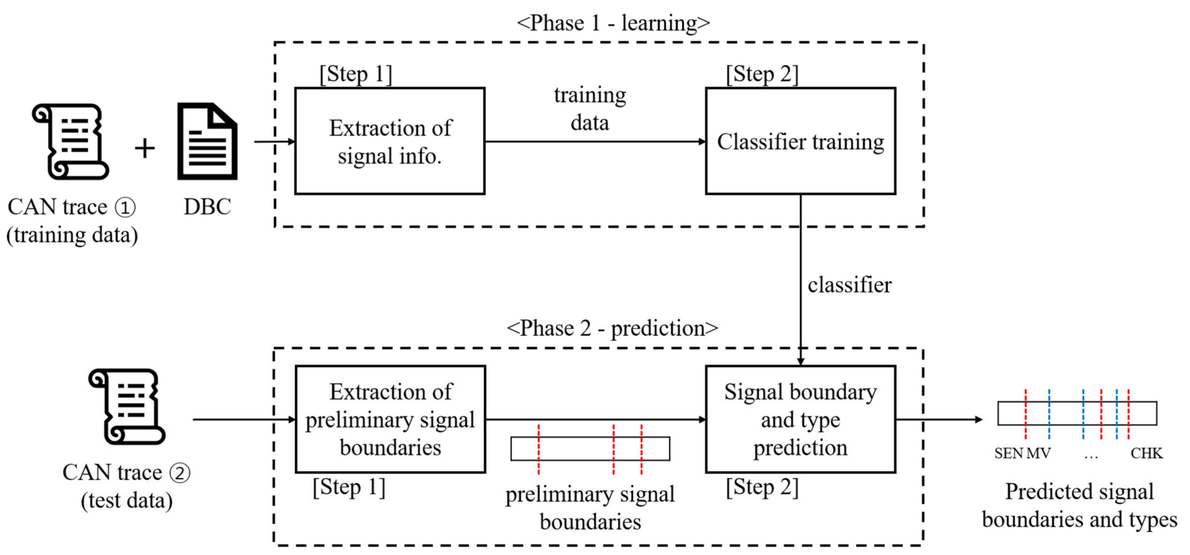
CA-CRE is based on the characteristics of signals, which can be divided into several distinguishable types. Time-series data extracted from a signal in chronological order have specific features, depending on the type of signal. For example, values of COUNTER signals commonly increase by one in chronological order. MULTI-VALUE signals, such as gear signals, have the same values in two consecutive frames in most cases, and they have relatively few unique values. CA-CRE learns these signal features in advance through machine-learning algorithms and uses the model to predict the signal boundaries and types of target CAN traces. The overall process of CA-CRE is shown in Figure 1. In Phase 1, it extracts feature values from a CAN trace and a relevant DBC to generate training data, which results in a dataset where each row represents nine feature values of a signal and a label of signal type. Then, the training data are provided to a classification model to train a classifier. In Phase 2, actual reverse-engineering is performed on a target CAN trace. First, preliminary signal boundaries are extracted from the trace. This process is the same as Phase 1 of the READ algorithm. Then, the classifier derived in Phase 1 is used to predict the boundaries and types of signals that reside between the preliminary signal boundaries. Details of each phase are described in the subsequent sections.
3.2. Phase 1—Training a Classifier
3.2.1. Signal Types
CA-CRE categorizes signals into six types: CONST, SENSOR, COUNTER, MULTI-VALUE, CHECKSUM, and WRONG. The signal types are inspired mainly by previous works [11,12,17], except the WRONG type. They aim to categorize most of the signals observed in real-world CAN data. Each signal type shows distinguishable characteristics. A description of the signal types is as follows:
- CONST signals refer to signals whose values are fixed in the entire trace. Ranges classified as CONST in CAN payloads are either undefined areas or signals that are rarely used, and they are both categorized as CONST since they are undistinguishable solely by observing traces.
- SENSOR signals contain physical data generated by ECUs, which show small differences between consecutive values (e.g., vehicle speed and RPM). Given that CAN messages of an arbitration ID generally have short inter-frame intervals (10–100 ms), differences between values of SENSOR signals such as RPM and vehicle speed are physically limited [11]. Thus, bit-flip rates of a SENSOR signal are likely to increase from MSB to LSB. The bit-flip rate of a specific bit-position is calculated by the number of bit-flips (0 to 1 and vice versa) of the bit-position between consecutive messages, divided by the number of the entire messages.
- COUNTER signals contain values that increase by a fixed value. The values generally increase by one, but sometimes they increase by a non-one value, depending on car manufacturers and models. There also exist COUNTER signals, which skip one or more values, and signals that enumerate random sequences of numbers repeatedly.
- MULTI-VALUE signals have values that change occasionally. They also have a relatively smaller number of unique values in the entire CAN trace. Signals containing information about the gear and the locking status of vehicle doors can be classified as the MULTI-VALUE type.
- CHECKSUM signals refer to signals that include checksum values for validating the integrity of a frame. Two consecutive values of a CHECKSUM signal generally have little correlation.
- WRONG signals denote signals that are not defined in DBC. This special type provides information on incorrect signals to classifiers so that they can distinguish between one of the five “RIGHT” signals above and incorrect signals.
The signal types are class labels of the samples in the dataset to train a classifier. While the feature values of a sample can be extracted automatically, the signal type of each sample is labeled manually by considering the name and observing the pattern of the time-series values of a corresponding signal.
3.2.2. Features
CA-CRE leverages nine features to quantify the characteristics of signals. Given that signals show distinct characteristics that can be classified as their types, the feature values extracted from real-world CAN traces are used to form a dataset to train a classifier. Details of the features are as follows:
- Size (bits): Each signal type has its own distribution of signal sizes. For example, 16-bit SENSOR signals are common, whereas the same size of CHECKSUM, COUNTER, and MULTI-VALUE signals are rarely found. Although it is difficult to predict types of given candidate fields based solely on their size, a combination of size and the other features can improve the accuracy of prediction.
- Minimum and maximum value: The maximum and minimum values are the largest and smallest values that a signal has shown in the entire trace. Patterns of minimum and maximum values of signals vary by their types. For example, the sizes of SENSOR signals are generally set larger than the exact size that contains the sensor values, whereas n-bit COUNTER signals generally have a minimum of 0 and maximum value of 2n − 1. WRONG signals also have different patterns concerning minimum and maximum values. For an 8-bit candidate field, where the first four bits are COUNTER signals and the remaining bits are the four most significant bits of another SENSOR signal that are not used, its minimum value is 0 and maximum value is 240, which are not common for 8-bit signals.
- Number of unique values: This self-explanatory feature also implies the type information of signals. SENSOR, COUNTER, and CHECKSUM signals have a relatively large number of unique values compared to MULTI-VALUE signals.
- Mean of differences and standard deviation of differences: For the entire sequence of values of a signal, the differences between adjacent values are calculated, and the mean and standard deviation of the differences are derived. Specifically, for the values vi obtained by interpreting the bitstring of signal s as an integer in the entire trace, the sequence of differences Ds of the signal is as follows: Ds = (v2 − v1, v3 − v2, …, vn − vn−1). These features aim to quantify patterns of fluctuation of signal values.
- Entropy/size: The minimum number of bits required to represent values included in a signal can be calculated with Shannon’s entropy [19]. Dividing the entropy value by the size (bits) of the signal yields a value between 0 and 1. If this indicator is close to 1, then all values that a signal can represent appear evenly. If it is close to 0, then values tend to be biased toward only part of the values that a signal can represent. For example, if a 4-bit signal is observed 1600 times in the entire trace, and all values from 0 to 15 appear equally 100 times, then the entropy/size of the corresponding signal is 1. This indicator is expected to be high in the order of MULTI-VALUE, SENSOR, CHECKSUM, and COUNTER. The formula for Shannon’s entropy is shown in Equation (1):For a sequence Vs = (v1, v2, …, vN) (0 < N) of all the values appearing in a signal s in chronological order, xi is calculated as Equation (2):xi = (the number of occurrences of vi)/N
- Fluctuation rate: Fluctuation rate (FR) is an index defined to quantify fluctuation of the values of a signal. The calculation formula of FR for a signal s is shown in Equation (3), where V is the sequence of values appearing in a signal, vi is the i-th value of the sequence, and N is length of V.FR is a normalized index of mean of differences by length of signals. FR is between 0 and 1, where an FR close to 0 means signal values are continuous throughout the trace and an FR close to 1 means the differences between adjacent values of a signal are large. If FR is exactly 1, then the corresponding l-bit signal’s values repeat 0 and 2l − 1.
- Flip-rate index: Flip-rate index (FRI) aims to quantify the frequency of signal-flip. Signal-flip means all the bits of a signal change from 1 to 0. Given that k is the number of signal-flip and l is the length of the corresponding signal, the formula for the flip-rate index is shown in Equation (4).The FRI is intended to differentiate between typical COUNTER and the other signal types. The FRI of a COUNTER signal that repeatedly increases by 1 from 0 to 2l − 1 is 1, or at least close to 1, if an adequate number of messages are given. By contrast, the FRI of SENSOR and MULTI-VALUE signals is inevitably close to 0. The FRI of CHECKSUM signals tend to be higher than that of SENSOR and MULTI-VALUE signals.
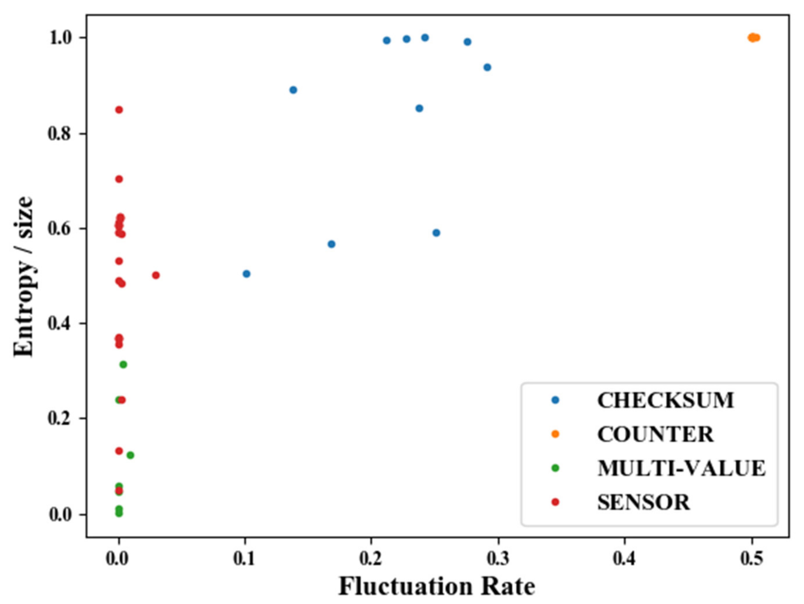
A combination of the features defined above can be used to differentiate between signal types. Figure 2 illustrates the FR‒entropy/size distribution of four types of signals from a real-world vehicle. FRs of the CHECKSUM signals are between 0.1 and 0.3. SENSOR and MULTI-VALUE signals exhibit low FR values, where the entropy/size values of SENSOR signals are generally larger than those of MULTI-VALUE signals. COUNTER signals show FRs of 0.5 or higher, because all COUNTER signals in the vehicle are 2-bit long. Intuitively, COUNTER signals seem to have lower FR values than CHECKSUM signals, but small-sized COUNTER signals have high FR values since the FR of an n-bit counter is 1/2n−1. Although there exist SENSOR signals that have lower entropy/size values than some of MULTI-VALUE signals, all four signal types are grouped together by the two features. Using the data above, the types of some unknown signals can be predicted. For example, if the FR of a signal is 0.001 and the entropy/size is 0.5, then the signal can be predicted to be a SENSOR signal. If a signal’s FR is 0.3 and the entropy/size is 0.99, the signal is highly likely to be CHECKSUM signal.
3.2.3. Classifier
CA-CRE leverages a supervised multiclass classification algorithm to predict the type of a given signal automatically upon its feature values. Supervised multiclass classification algorithms aim at assigning a class label for each input sample. Given training data of the form (xi, yi), where xi is the ith sample and yi ∈ {l1, …, lk} (k > 2) is the ith class label, the algorithms aim at finding a learning model M, such that M(xi) = yi for new unseen samples [20]. There exist various types of multiclass classification algorithms, such as neural networks, decision trees, k-nearest neighbor, naive Bayes, and support vector machines. Appropriate algorithms for CAN signal prediction can vary depending on the features chosen, the number of class labels, and the size of training data. In this work, the most appropriate algorithm is proposed by experiments on the datasets from a real-world CAN trace and synthetic CAN traces. Details on the selection of the classification algorithm used in this work are described in Section 4.3.
3.2.4. Training Data
The training data are included in a table, where each row contains the feature values of a signal as defined in Section 3.2.2 and a label that represents the type of the signal. Specifically, feature values for each signal defined in a DBC are calculated from a corresponding CAN trace to form X = (x1, …, xN), and a signal type that corresponds to each xi is assigned to form Y = (y1, …, yN). X and Y establish training data, where each xi contains nine feature values of a signal and yi ∈ {SENSOR, MULTI-VALUE, COUNTER, CRC, WRONG}. CONST signals are not included in the training data because they can be identified without a classifier.
In the training data, not only normal signals existing in the DBC but also WRONG-type signals that are intentionally misidentified signals are collected. They are intended for a classifier to learn misidentified signals. WRONG-type signals are generated in two ways, as follows:
- Signals that are 1 or 2 bits larger to the right-hand side than the existing signals:
- For each existing signal s whose range is (pos_ls, pos_rs), where pos_l (0 ≤ pos_ls< 64) is the leftmost bit position of signal s and pos_r (0 ≤ pos_rs < 64) is the rightmost bit position of signal s, two WRONG signals with positions of (pos_ls, pos_rs + 1) and (pos_ls, pos_rs + 2) are added to the training data if the signals are within the range of their payload.
- Signals that are a concatenation of two or three consecutive existing signals:
- For all signals s1 and s2, such that pos_rs1 + 1 = pos_ls2, WRONG signals with positions of (pos_ls1, pos_rs2) are newly added to the training data.
- For all signals s1, s2, and s3, such that pos_rs1 = pos_ls2 and pos_rs2 = pos_ls3, WRONG type signals with positions of (pos_ls1, pos_rs3) are added to the training data.
Generating WRONG-type signals as above is related to the manner in which the classifier is used in the signal boundary prediction described in Section 3.3.2. In Step 2 of Phase 2, a candidate field is given to a classifier, asking whether it is a RIGHT signal or not. If the classifier’s answer is WRONG, then the size of the candidate field decreases by 1 from the right-hand side, until the classifier predicts a RIGHT signal. Thus, adding WRONG signals that are 1 or 2 bits larger to the right-hand side than the existing signals is expected to provide effective information to a classifier for more accurate prediction.
3.3. Phase 2—Signal Boundary and Type Prediction
In Phase 2, boundaries and types of signals are predicted by utilizing the previously derived classifier. Phase 2 is composed of two steps: extraction of preliminary signal boundaries and prediction of signal boundary and type.
3.3.1. Extraction of Preliminary Signal Boundaries
In the first step of Phase 2, CA-CRE first extracts preliminary signal boundaries in the data field for each ID in a target CAN trace. This process is identical to the preprocessing phase and Phase 1 of READ [11]. CA-CRE first computes bit-flip rates for each TIDi (0 < i ≤ n) of the entire CAN trace T = {TID1, …, TIDn} and derives the magnitude array based on the bit-flip rates. The formula for the j-th bit-flip rate of IDi is shown in Equation (5), where Fj is the number of times the j-th bit is flipped in TIDi, and |TIDi| is the total number of messages of IDi.
Calculating the magnitude array using the bit-flip rate is performed as shown in Equation (6), where Mi is the i-th element of the magnitude array and Bi is the bit-flip rate of the i-th bit.
After the magnitude array is derived, the magnitude array of each IDi is observed to derive the preliminary signal boundaries PIDi for TIDi. The algorithm observes the magnitude values Mj and Mj+1 of two consecutive bits, and if Mj is greater than Mj+1, then the boundary between the two bits is added to PIDi.
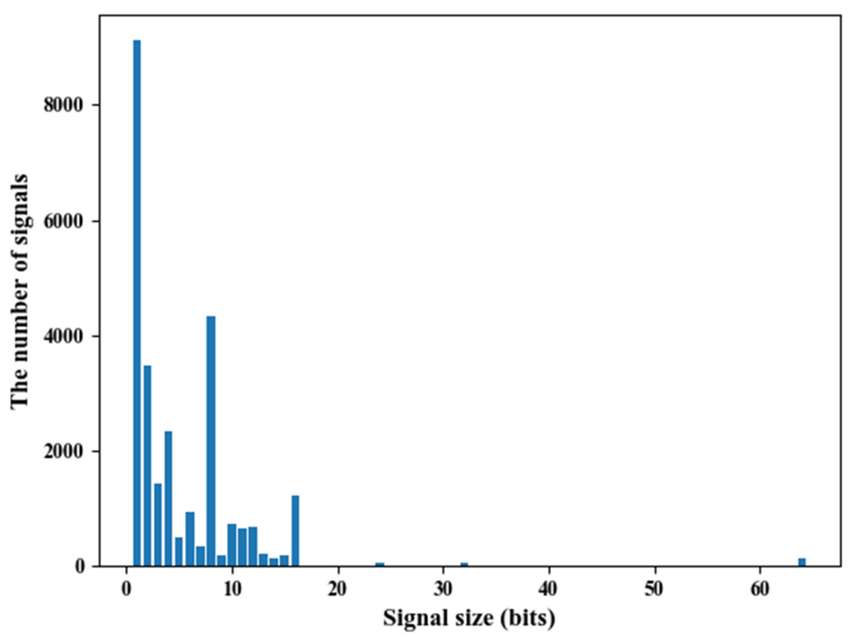
CA-CRE has two motivations to establish a preliminary signal boundary before using a classifier. First, the preliminary signal boundaries show a relatively higher precision than the signal boundaries predicted by other reverse-engineering algorithms. Table 1 shows the precision and recall values of the three algorithms (READ Phase 1, READ, and LibreCAN Phase 1). True positive (TP) means that a boundary identified by a reverse-engineering algorithm is a signal boundary. A false positive (FP) is a case when a boundary identified by an algorithm is not an actual signal boundary. A false negative (FN) is a case where a boundary not identified by an algorithm is an actual signal boundary. READ Phase 1 has lower TP than READ and LibreCAN but also has lower FP, resulting in high precision. That is, READ Phase 1 finds fewer points that are actual boundaries, whereas the probability that the boundaries it identified are actual boundaries is relatively high. In the real-world CAN trace, READ Phase 1 shows slightly lower precision than READ. However, the number of FPs in both is the same, and this is attributed to the fact that no FP occurs when READ identifies seven more boundaries in the result of READ Phase 1. Structurally, READ and LibreCAN include READ Phase 1 (LibreCAN uses a slightly different version); thus, the FP of READ Phase 1 is lower than or equal to that of the other two algorithms. Second, given that signals larger than 16 bits are rarely found (as shown in Figure 3), using a classifier for a small range is more efficient and accurate than using a classifier to find signals from scratch because READ phase 1 separates the entire payload into a few sections in a reliable manner.
3.3.2. Signal Boundary and Type Prediction
In the second step of Phase 2, CA-CRE uses preliminary boundaries and classifiers to determine the final signal boundaries and types. First, the algorithm divides the entire data field into smaller detailed fields based on the preliminary boundaries of PIDi. For example, if ID1’s DLC is 2 and the preliminary boundaries are found between the 4th and 5th bits and between the 12th and 13th bits, the subfields of PID1 are {(0, 4), (5, 12), (13, 15)}. The algorithm then repeatedly asks the classifier for the signal type of the current range until RIGHT signals are predicted, thereby decreasing pos_r by 1 for each subfield (pos_l, pos_r). If no RIGHT signals are found until the last two bits, the entire subfield is determined as a WRONG signal. If the classifier predicts a specific range as a RIGHT signal, then the corresponding range is finally determined as a signal, and the process is repeated for the remaining part. The pseudocode for the signal determination algorithm used in Step 2 is shown in Algorithm 1.
| Algorithm 1. Predict_subfields |
| function predict_subfields(start, end, bfrs, clf) res ← list() length ← end − start + 1 if length < 2 then return [(start, end, ‘one-bit’)] for size in range(length..1) do pos_l ← start pos_r ← pos_l + size − 1 # case 1: const if all BFRs are 0 in the range of (pos_l..pos_r) then res.append ((start, pos_r, ‘const’)) if pos_r < end then res.extend(predict_subfields(pos_r+1, end, bfrs, clf)) return res # case 2: match X ← get_features(pos_l, pos_r) y ← clf.predict(X) if y ≠ ‘wrong’ then res.append((pos_l, pos_r, y)) if pos_r < end then res.extend(predict_subfields(pos_r+1, end, bfrs, clf)) return res # case 3: no match res.append((start, end, ‘wrong’)) return res |
4. Performance Evaluation
4.1. Datasets
CA-CRE is evaluated on two datasets. The first dataset contains synthetic signal information of CAN traces generated on a simulated CAN bus, and the second dataset has signal information extracted from a real-world vehicle’s CAN trace [15] and DBC [13], which can be obtained through the internet. The synthetic CAN dataset is used for experiments on a large amount of data with reliable signal information. The synthetic CAN traces are generated through a CAN trace generator written in Python. Table 2 shows a detailed composition of the traces. Seven different traces are generated, five of which are for training data, and two for test data. Each CAN trace has approximately three million CAN frames collected for 500 s on a CAN bus that 60 ECUs have transmitted with different arbitration IDs at 10 ms intervals. Each message has 8 bytes of DLC, and the format of its data field is randomly determined. A total of 3786 signals is included in the five traces, and the final training data consist of 11,735 records by adding the information of 7946 WRONG signals. The remaining two traces contain 1552 signals, and the final test data consist of 4782 records by adding the information of 3230 WRONG signals.
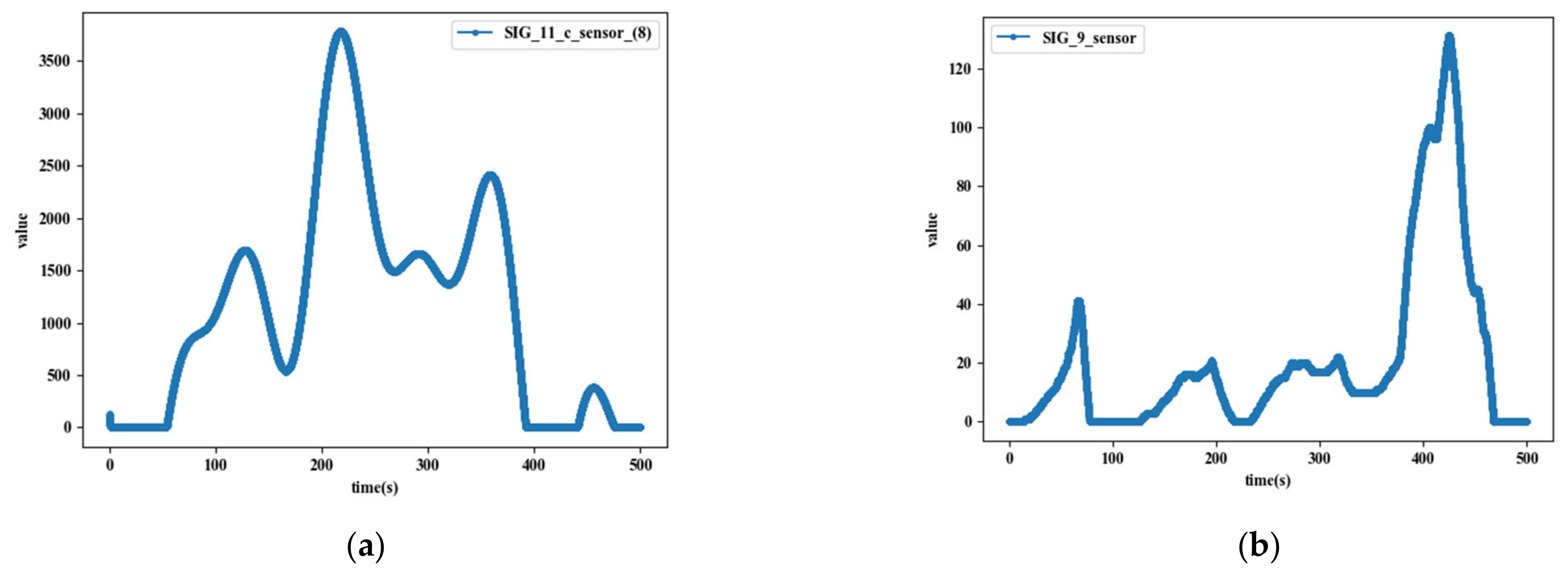
Table 3 outlines how the signals in the synthetic CAN dataset are generated. A CONST signal has a fixed value throughout the entire trace. A MULTI-VALUE signal has a value of 0 in most cases and shows a value greater than 0 with a small probability. A COUNTER signal has a pattern that starts from an arbitrary value and increases by 1, and when the value reaches a certain number, it returns to 0 and increases again by 1. A CRC signal always has arbitrary values. SENSOR signals have two types. A Type-1 SENSOR signal simulates SENSOR values based on a composite sine function. The individual sine function of the composite sine is arbitrarily selected within a certain range of amplitude, period, phase, and base, and the final value of the signal is created by adding these multiple sine values. Type-2 is intended to produce a sequence of values different from the composite sine function, which is assumed to add more diversity to the synthetic CAN traces. The (i + 1)th value of a Type-2 SENSOR signal is determined by adding delta to the i-th value. The delta changes continuously through the product of a random sample of standard normal distribution and a factor (a parameter to adjust the degree of change). Given that signal values may increase or decrease excessively when the delta is too biased, the delta is adjusted with a certain probability if the increase or decrease of the values continues over a certain number of times (for example, 1000 times). Figure 4 illustrates examples of synthetic SENSOR Type-1 and Type-2: (a) shows the values of an 8-bit SENSOR Type-1 signal and (b) shows the values of an 11-bit SENSOR Type-2 signal over time.
The real-world CAN trace contains approximately 1.8 million CAN frames generated from a CAN bus of a sedan released in 2016. The corresponding DBC contains signal information of 56 IDs, and only 27 of them appear on the trace. Among the signals included in the 27 IDs, 52 signals are used for training, excluding CONST and 1-bit signals. Table 4 shows an example of signals defined in a single CAN ID. Among the 11 signals, two SENSOR signals, one COUNTER signal, and one CHECKSUM signal are included in the dataset. The rest are not defined in the DBC, are too small to learn (ONE-BIT), or are not needed for training because they always show a fixed value. Table 5 shows the number of signals included in the dataset in terms of their signal type and the number of CAN IDs containing those signals. Given that only four IDs contain MULTIVALUE signals, the entire dataset is divided into four folds, so that each fold contains at least one sample of a MULTI-VALUE signal.
4.2. Performance Metrics
In previous works [11,12], the performance of READ is measured through comparison with FBCA [17] in terms of the number of extracted signals, and the performance of LibreCAN Phase 0 is presented by the ratio of correctly extracted signals to all signals in DBC. Performance measurements from these previous studies mainly consider exactly extracted signals. However, performance on strict metrics is not always the only meaningful result because the purpose of reverse engineering may vary depending on how the results are utilized. For example, reverse-engineered signal information can be used for intrusion detection, as shown in [17], or it can be used for security testing through the penetration test or fuzzing on the vehicle’s internal network. In these cases, not only perfectly matched results but also mismatched results that are close to ground truth are more useful than completely incorrect results.
In this work, the performance of CAN signal reverse-engineering methods is measured by mapping their results into several match types. Table 6 describes detailed match conditions for each match type. Each signal is expressed in the form of (l, r, t), where l, r, and t mean the position of the left bit, the position of the right bit, and the signal type of the corresponding signal, respectively (0 ≤ l < DLC ∙ 8, 0 ≤ r < DLC ∙ 8, t ∈ {‘CONST’, ‘MULTI-VALUE’, ‘COUNTER’, ‘SENSOR’, ‘CHECKSUM’}). The match types consist of best match, effective match, and partial match. Examples of match types are also depicted in Table 7. Best match means both boundaries of a predicted signal are identical to those defined in DBC, which is the same metric as used in the existing studies. Effective match is intended to cover the cases that are mismatched because of adjacent CONST signals. For example, if the left signal of a SENSOR signal has a fixed value only, it is difficult to find out the exact length of the SENSOR signal due to lack of information. The partial match is intended to quantify the tendency of incorrect prediction results. Algorithms that show relatively large numbers of match type 2.1 tend to split signals into pieces smaller than the ground truth. Conversely, a large number of type 2.2 implies a tendency for the algorithm to predict signals larger than ground truth. Type 2.3 is assigned to signals that do not correspond to all match types from type 0 to type 2.2. All match types are counted based on the signals in DBC. For a match of type 1.2, for instance, a single signal is predicted, but it is counted as two T1,2 matches because it corresponds to two signals in DBC. Lastly, some DBC signals may not belong to any match type, although this does not occur when the DBC information is complete. It happens when undefined areas exist. The number of signals that do not belong to any type is expressed as T’ or no_match.
To measure the performance of CAN reverse-engineering algorithms, two metrics are defined based on the match types, as follows:
- P1 = |T0|/(|T0|+|T1|+|T2|+|T’|)
- P2 = (|T0|+|T1|)/(|T0|+|T1|+|T2|+|T’|)
The sum of |T0|, |T1|, |T2|, and |T’| is the number of all signals of the corresponding CAN ID. P1 means the ratio of correctly identified signals to the total signals. P2 refers to the ratio of correctly identified signals and effectively identified signals to the total signals. In addition to P1 and P2, two other indicators are defined as follows to indicate the tendency of signals predicted by a reverse-engineering algorithm.
- P3 = |T2,1|/|T2|
- P4 = |T2,2|/|T2|
P3 represents the proportion of signals predicted as smaller pieces than the ground truth among all the signals that the algorithm incorrectly predicted. Conversely, P4 represents the proportion of the signals predicted to be larger than the actual signal to the signals incorrectly predicted. Algorithms with a higher P3 tend to show relatively high recall by predicting signal boundaries aggressively at the expense of lower precision, whereas algorithms with a higher P4 tend to show higher precision and lower recall by determining, only relatively, certain boundaries as final signal boundaries.
4.3. Comparison of Classification Algorithms
A classification algorithm is used to predict the final signal boundary and type within predetermined preliminary signal boundaries. To find the most suitable algorithm among various classification algorithms, auto-sklearn [21,22], a tool to help select an appropriate algorithm and parameter tuning, is utilized first. Then, the results of auto-sklearn are further refined via cross-validation to select the best algorithm. A script for comparison is written in Python, and all the implemented machine-learning algorithms are based on scikit-learn [23]. Cross-validation (CV) is performed separately on the synthetic CAN dataset and the real-world CAN dataset. For the synthetic dataset, five-fold CV is applied to the training data, and the final performance result is measured by the test data. In the real CAN dataset, four-fold CV is applied to distribute each signal type to every fold, as mentioned in Section 4.1. The final performance result is determined by averaging the CV results.
Table 8 shows the performance results of algorithms with 0.9 or higher accuracy among a total of 278 parameter settings of 15 different algorithms tested by auto-sklearn. Although each algorithm has multiple parameter settings, only the highest score of each algorithm is tested. The algorithms listed in Table 8 are also cross-validated on both the synthetic dataset and real-world dataset. The third and the fourth column of Table 8 show cross-validation results for the synthetic and real-world datasets, respectively. As shown in the table, the algorithm that shows the best performance for both datasets is random forest, whose accuracy scores are 0.971 for the synthetic dataset and 0.869 for the real-world dataset. Based on this result, CA-CRE leverages random forest as its classification algorithm. The parameters used in the algorithm are shown in Table 9.
4.4. Comparison of CAN Reverse—Engineering Algorithms
A comparative experiment is performed on READ phase 0, READ, LibreCAN (Phase 0), and CA-CRE on the synthetic CAN traces and the real-world CAN trace. READ phase 0 is included in this experiment since it is used as a preprocessing step of READ, LiberCAN, and CA-CRE. LibreCAN consists of three phases (Phase 0 to Phase 2), and Phases 1 and 2 improve the results from Phase 0 through additional channels other than CAN trace; hence, it is difficult to compare between LibreCAN Phase 1/2 and the other algorithms. Therefore, only LibreCAN Phase 0 is used for comparison. READ and LibreCAN are implemented as described in the pseudocode of each literature, and scripts of the algorithms are written in Python. Experiments are performed on a laptop with a Windows 10 (64 bits) operating system, Intel Core i7 1.8 GHz CPU, and 16 GB RAM.
4.4.1. Performance on Synthetic CAN Dataset
As mentioned in Section 4.1, the synthetic CAN trace consists of a total of seven CAN traces, where five of them are used as training data and two of them are used as test data. Each trace contains approximately 3 million CAN frames. READ and LibreCAN are performed on the test data. CA-CRE first generates a random forest classifier using signal information extracted from the training data and then is performed on the test data.
Table 10 shows the experiment results of the four algorithms on the synthetic CAN dataset. n_signal represents the number of signals predicted by each algorithm, and the number of signals in DBC is 1552. no_match denotes the number of DBC signals that do not correspond to any match type. Table 10 also includes the number of match types extracted by the algorithms and the performance results derived using them. Given that match types are counted by signals defined in DBC, the sum of all the match types and no_match of each algorithm are always identical to the number of signals defined in DBC. Based on P1 and P2, the performance of the reverse-engineering algorithms on the synthetic CAN dataset is high, in the order of CA-CRE, READ, LibreCAN, and READ Phase 1. READ outperforms LibreCAN in this dataset. LibreCAN Phase 0 works almost the same as READ, but by altering conditions of signal boundary decision, it tends to determine signal boundaries more aggressively than READ. Therefore, the number of signals extracted by LibreCAN is larger than that of others. In addition, P3 of LibreCAN is relatively higher, and P4 is lower than others, indicating that LibreCAN predicts signals as multiple smaller signals than READ due to the relaxed boundary identification conditions.
Both CA-CRE and READ first identify preliminary signal boundaries through READ Phase 1 and then predict the detailed signals existing between the preliminary boundaries. However, the two algorithms show different results from the intermediate result (713 signals of READ Phase 1 match type 2.2 are further divided into smaller signals by the two algorithms). READ reduces the number of match type 2.2 from 713 to 401, whereas CA-CRE reduces them to 222. After the post-process, CA-CRE achieves higher P1 and P2 at the cost of a slightly larger number of match type 2.1 and 2.3 compared to READ.
4.4.2. Performance on Real-World CAN Dataset
Table 11 shows the performance results of the four algorithms on the real CAN dataset. The result indicates that CA-CRE also outperforms the other algorithms on the real-world dataset. P1 of CA-CRE is 0.460, which is at least 0.12 higher than that of LibreCAN and 0.17 higher than that of READ. P2 of CA-CRE is slightly higher than that of the others, and it is assumed that the result is due to the size of the training data. The total number of samples in the real-world dataset is 52, and a classifier is trained with only 39 samples in each fold during cross-validation (The total number of signals defined in the real-world DBC is 127, and 52 of them are contained in the dataset, excluding CONST and 1-bit signals).
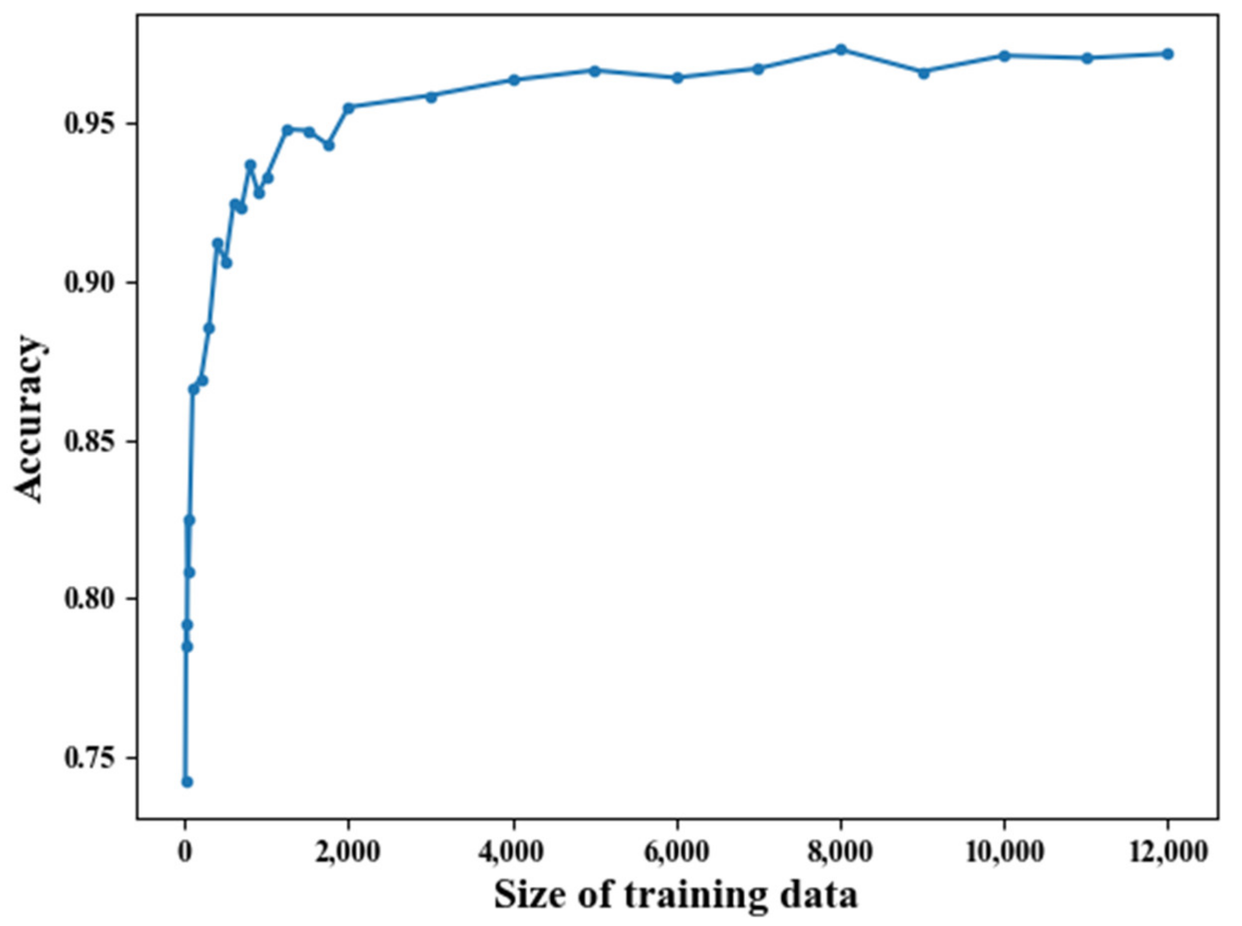
To estimate how sufficient the real-world dataset is, an additional experiment is performed by measuring accuracies of a classifier with different sizes of training data. Figure 5 shows the accuracies of a random forest classifier with different sizes of training data. The parameters of the classifier are identical to Table 9. For each size, training data are provided to the classifier by random sampling. Accuracy is measured on all the 4782 test data, regardless of the size of the training data. When the data size is 30 or less, accuracies are 0.8 or less. When the data size is approximately 2000 or more, accuracies are more than 0.95. This result suggests that at least 2000 samples of data should be provided to obtain the best performance from a classifier. Therefore, it can be interpreted that CA-CRE outperforms the previous works with only a limited number of samples (39 samples in this experiment) of training data.
5. Discussion
As the experimental results suggest, CA-CRE shows better reverse-engineering performance than the existing methods. However, the proposed method also has a limitation; an adequate amount of training data must be provided. To overcome this limitation, one can utilize the DBCs that are already reverse-engineered by researchers and accessible through the internet [13]. In addition, if a large amount of training data from various types of real-world vehicles is accumulated with additional features (manufacturers, vehicle models, vehicle types, etc.), the method can be improved to reverse-engineer for unseen vehicles’ CAN payload format. Once signal data from various types of vehicles are gathered, a classifier that is trained with the data is expected to predict signals of an unseen vehicle because DBC has strict rules that each signal must have min, max, scale, offset, etc. These characteristics ensure that different vehicle models have similar signals even though they have different formats. CA-CRE can also be improved by considering sign and endianness in future works. Currently, the method requires users to select endianness in advance, and if an input trace is in little-endian format, it is read after payloads are converted into big-endian. The values of signals are also interpreted as unsigned integers and thus could lead to misidentification of signed signals. To summarize, larger datasets that are collected from various types of vehicles will be used, with additional features and endian-awareness in future work.
The CAN reverse-engineering method itself could be considered as a threat to in-vehicle network security since it also provides format information to attackers. However, securing the format information is regarded as the security through obscurity paradigm. It may delay attacks, but the format information can be revealed by the attackers eventually. Automatic reverse-engineering methods may disclose format information, but can strengthen network security tests performed by evaluation authorities and third-party researchers.
6. Conclusions
In this paper, we proposed CA-CRE, a reverse-engineering method that predicts signal boundaries from CAN traces. CA-CRE utilizes a classification algorithm to find similar signals on the basis of previously learned signal information. Training data include information on previously known signals as well as intentionally misclassified signal information based on ground truth.
The reverse-engineering performance of the algorithms, including CA-CRE and previous works [11,12], was evaluated on a synthetic CAN dataset and a real-world CAN dataset. Several new metrics were defined to measure practical performance of the algorithms. The experimental results showed that the proposed method can predict signal boundaries more accurately than existing algorithms on both datasets.
Given that the machine-learning technique used in CA-CRE is a supervised learning method, there exists a precondition that some ground truth must be acquired in advance of reverse-engineering. Nevertheless, this limitation can be overcome in several ways. Once enough training data are obtained, CA-CRE can contribute to reducing the manual reverse-engineering effort by researchers who study CAN security technology and improving the performance of automated security testing for IVN.
Author Contributions
All authors contributed to this work. Conceptualization, C.J.; methodology, C.J.; software, C.J.; validation, C.J., T.K. and M.H.; writing—original draft preparation, C.J.; writing—review and editing, T.K.; visualization, C.J.; supervision, M.H.; project administration, M.H. All authors have read and agreed to the published version of the manuscript.
Funding
This research received no external funding.
Acknowledgments
This research was supported by the Korea Ministry of Land, Infrastructure and Transport. It was also supported by the Korea Agency for Infrastructure Technology Advancement (Project No.: 21PQOW-B152473-03).
Conflicts of Interest
The authors declare no conflict of interest.
References
- Miller, C.; Valasek, C. Remote Exploitation of an Unaltered Passenger vehicle. Black Hat USA, Las Vegas, NV, USA, 1–6 August 2015. Available online: https://www.academia.edu/download/53311546/Remote_Car_Hacking.pdf (accessed on 17 September 2021).
- Kamkar, S. Drive It Like You Hacked It: New Attacks and Tools to Wirelessly Steal Cars. DEF CON 23, Las Vegas, NV, USA, 6–9 August 2015. Available online: https://samy.pl/defcon2015/ (accessed on 17 September 2021).
- Miller, C.; Valasek, C. Advanced CAN Injection Techniques for Vehicle Networks. Black Hat USA, Las Vegas, NV, USA, 4 August 2016. Available online: http://illmatics.com/can%20message%20injection.pdf (accessed on 17 September 2021).
- Garcia, F.D.; Oswald, D.; Kasper, T.; Pavlidès, P. Lock it and still lose it–on the (in) security of automotive remote keyless entry systems. In Proceedings of the 25th USENIX Security Symposium (USENIX Security 16), Austin, TX, USA, 10–12 August 2016; pp. 929–944. [Google Scholar]
- Nie, S.; Liu, L.; Du, Y. Free-Fall: Hacking Tesla from Wireless to Can Bus. Black Hat USA, Las Vegas, NV, USA, 22–27 June 2017. Available online: https://www.blackhat.com/docs/us-17/thursday/us-17-Nie-Free-Fall-Hacking-Tesla-From-Wireless-To-CAN-Bus-wp.pdf (accessed on 17 September 2021).
- Milburn, A.; Timmers, N.; Wiersma, N.; Pareja, R.; Cordoba, S. There Will Be Glitches: Extracting and Analyzing Automotive Firmware Efficiently. Black Hat USA, Las Vegas, NV, USA, 4–9 August 2018. Available online: https://www.riscure.com/uploads/2018/11/Riscure_Whitepaper_Analyzing_Automotive_Firmware.pdf (accessed on 17 September 2021).
- Lynch, K.M.; Marchuk, N.; Elwin, M. Embedded Computing and Mechatronics with the PIC32 Microcontroller, 1st ed.; Newnes: Waltham, MA, USA, 2015; Chapter 19; pp. 249–266. ISBN 978-012-420-235-1. [Google Scholar]
- 5 Advantages of CAN Bus Protocol. Available online: https://www.totalphase.com/blog/2019/08/5-advantages-of-can-bus-protocol/ (accessed on 8 September 2021).
- Comparison of CAN Bus and Ethernet Features for Automotive Networking Applications. Available online: https://copperhilltech.com/blog/comparison-of-can-bus-and-ethernet-features-for-automotive-networking-applications/ (accessed on 8 September 2021).
- Richards, P.A. CAN Physical Layer Discussion. Available online: http://ww1.microchip.com/downloads/en/AppNotes/00228a.pdf (accessed on 8 September 2021).
- Marchetti, M.; Stabili, D. READ: Reverse engineering of automotive data frames. IEEE Trans. Inf. Forensics Secur. 2018, 14, 1083–1097. [Google Scholar] [CrossRef]
- Pesé, M.D.; Stacer, T.; Campos, C.A.; Newberry, E.; Chen, D.; Shin, K.G. LibreCAN: Automated CAN message translator. In Proceedings of the 2019 ACM SIGSAC Conference on Computer and Communications Security, London, UK, 11–15 November 2019; pp. 2283–2300. [Google Scholar]
- Opendbc. Available online: https://github.com/commaai/opendbc (accessed on 8 September 2021).
- ISO/SAE 21434:2021 Road vehicles—Cybersecurity Engineering. Available online: https://www.iso.org/standard/70918.html (accessed on 8 September 2021).
- Comma Cabana. Available online: https://my.comma.ai/cabana/?demo=1 (accessed on 8 September 2021).
- DBC Format. Available online: http://socialledge.com/sjsu/index.php/DBC_Format (accessed on 8 September 2021).
- Markovitz, M.; Wool, A. Field classification, modeling and anomaly detection in unknown CAN bus networks. Veh. Commun. 2017, 9, 43–52. [Google Scholar] [CrossRef]
- Verma, M.E.; Bridges, R.A.; Hollifield, S.C. ACTT: Automotive CAN tokenization and translation. In Proceedings of the IEEE International Conference on Computational Science and Computational Intelligence (CSCI), Las Vegas, NV, USA, 12–14 December 2018; pp. 278–283. [Google Scholar]
- Shannon, C.E. A mathematical theory of communication. Bell Syst. Tech. 1948, 27, 379–423. [Google Scholar] [CrossRef] [Green Version]
- Aly, M. Survey on multiclass classification methods. Neural Netw. 2005, 19, 1–9. [Google Scholar]
- Feurer, M.; Klein, A.; Eggensperger, K. Efficient and robust automated machine learning. Adv. Neural Inf. Process Syst. 2015, 28, 2962–2970. [Google Scholar]
- Feurer, M.; Eggensperger, K.; Falkner, S.; Lindauer, M.; Hutter, F. Auto-Sklearn 2.0: The Next Generation. Available online: https://arxiv.org/abs/2007.04074 (accessed on 8 September 2021).
- Pedregosa, F.; Varoquaux, G.; Gramfort, A.; Michel, V.; Thirion, B.; Grisel, O.; Blondel, M.; Prettenhofer, P.; Weiss, R.; Dubourg, V.; et al. Scikit-learn: Machine learning in python. J. Mach. Learn. Res. 2011, 12, 2825–2830. [Google Scholar]
Figure 1.
Overall process of CA-CRE.

Figure 2.
Distribution of FR and entropy/size values by signal type.

Figure 3.
Distribution of sizes of all signals defined in the DBCs of OpenDBC [13].
Figure 3.
Distribution of sizes of all signals defined in the DBCs of OpenDBC [13].

Figure 4.
Examples of synthetic SENSOR Type-1 (a) and Type-2 (b).

Figure 5.
Accuracy of a classifier by the size of training data.


Table 1.
TP, FP, FN, precision, and recall of the three CAN reverse-engineering algorithms on a real car’s CAN trace and a synthetic CAN trace (both 1M messages).
Table 1.
TP, FP, FN, precision, and recall of the three CAN reverse-engineering algorithms on a real car’s CAN trace and a synthetic CAN trace (both 1M messages).
| CAN Trace | Metrics | READ Phase 1 | READ | LibreCAN |
|---|---|---|---|---|
| Real-world CAN trace | True Positive | 42 | 49 | 66 |
| False Positive | 4 | 4 | 31 | |
| False Negative | 75 | 68 | 51 | |
| Precision | 0.913 | 0.925 | 0.680 | |
| Recall | 0.359 | 0.419 | 0.564 | |
| Simulated CAN trace | True Positive | 395 | 485 | 508 |
| False Positive | 0 | 4 | 270 | |
| False Negative | 295 | 205 | 182 | |
| Precision | 1.0 | 0.992 | 0.653 | |
| Recall | 0.572 | 0.703 | 0.736 |
Table 2.
Composition of the synthetic CAN dataset.
| Data Type | Trace | Extracted Signal | ||||
|---|---|---|---|---|---|---|
| Trace Number | Frames | Total Frames | RIGHT Signals | WRONG Signals | Total Records | |
| Training data | 0 | 3,017,987 | 15,090,068 | 3789 | 7946 | 11,735 |
| 1 | 3,018,062 | |||||
| 2 | 3,018,136 | |||||
| 3 | 3,017,893 | |||||
| 4 | 3,017,990 | |||||
| Test data | 5 | 3,023,712 | 6,047,746 | 1552 | 3230 | 4782 |
| 6 | 3,024,034 | |||||
Table 3.
Signal types, range of signal size, and description of how they are generated on the synthetic CAN bus.
Table 3.
Signal types, range of signal size, and description of how they are generated on the synthetic CAN bus.
| Signal Type | Signal Size | Signal Value Description (n = Signal Size, 0 ≤ i < N) |
|---|---|---|
| CONST | 1 … 8 | |
| MULTIVALUE | 1 … 4 | |
| COUNTER | 4 … 6 | |
| CRC | 4 … 6 | |
| SENSOR (Type-1) | 6 … 8 | |
| SENSOR (Type-2) | 6 … 18 |
Table 4.
Example of signals included in a CAN ID of the real CAN trace.
| Signal Name | Signal Type | Length (Bits) |
|---|---|---|
| PEDAL_GAS | SENSOR | 8 |
| empty | NOT DEFINED | 8 |
| ENGINE_RPM | SENSOR | 16 |
| GAS_PRESSED | ONE-BIT | 1 |
| ACC_STATUS | ONT-BIT | 1 |
| BOH_17C | CONST | 5 |
| BREAK_SWITCH | ONE-BIT | 1 |
| BOH2_17C | CONST | 10 |
| BREAK_PRESSED | ONE-BIT | 1 |
| BOH3_17C | CONST | 5 |
| empty | NOT DEFINED | 2 |
| COUNTER | COUNTER | 2 |
| CHECKSUM | CHECKSUM | 4 |
Table 5.
Example of signals included in a CAN ID of the real CAN trace.
| Signal Type | Signals | IDs Containing the Signal Type |
|---|---|---|
| MULTI-VALUE | 7 | 4 |
| SENSOR | 26 | 12 |
| COUNTER | 9 | 9 |
| CHECKSUM | 10 | 10 |
Table 6.
Match conditions of match types.
| Match Type | Type Number | Mnemonic | DBC | Predicted Result | Match Conditions (Common Condition: l ≤ r for all (l, r, t)) |
|---|---|---|---|---|---|
| Best match | Type 0 | T0 | (l, r, t) | (l, r, t’) | |
| Effective match | Type 1.1 | T1,1 | (l, r, t) | (l, x, t1′), (x+1, r, t2′) | l < x < r, t1′ = CONST, t2′ ≠ CONST |
| Type 1.2 | T1,2 | (l, x, t1), (x+1, r, t2) | (l, r, t’) | l < x < r, t1 = CONST, t2 ≠ CONST | |
| Type 1.3 | T1,3 | (l, x, t1), (x+1, r, t2) | (l, y, t1′), (y+1, r, t2′) | l < x < r, l < y < r, x ≠ y, t1 = CONST, t2 ≠ CONST, t1′ = CONST, t2′ ≠ CONST | |
| Partial match | Type 2.1 | T2,1 | (l, r, t) | (l, x1, t1), (x1+1, x2, t2), … (xn+1, r, tn+1) | l < x1 < … < xn < r |
| Type 2.2 | T2,2 | (l, x1, t1), (x1+1, x2, t2), … (xn+1, r, tn+1) | (l, r, t) | l < x1 < … < xn < r | |
| Type 2.3 | T2,3 | (l, x1, t1), (x1+1, x2, t2), … (xn+1, r, tn+1) | (l, y1, t1), (y1+1, y2, t2), … (yn+1, r, tn+1) | l < x1 < … < yn < r, l < y1 < … < yn < r, {x1, …, xn} ∩ {y1, …, yn} = Ø |
Table 7.
Examples of match types.
| Match Type | Type Number | Examples |
|---|---|---|
| Best match | Type 0 |  |
| Effective match | Type 1.1 |  |
| Type 1.2 |  | |
| Type 1.3 |  | |
| Partial match | Type 2.1 |  |
| Type 2.2 |  | |
| Type 2.3 |  |
Table 8.
Performance results of auto-sklearn and cross-validation scores of classification algorithms on synthetic and real-world datasets.
Table 8.
Performance results of auto-sklearn and cross-validation scores of classification algorithms on synthetic and real-world datasets.
| Algorithm | Mean Test Score by Auto-Sklearn | Mean 5-Fold CV Score on the Synthetic Dataset | Mean 4-Fold CV Score on the Real Car Dataset |
|---|---|---|---|
| gradient boosting | 0.975 | 0.961 | 0.701 |
| random forest | 0.967 | 0.971 | 0.869 |
| adaboost | 0.966 | 0.781 | 0.734 |
| extra_trees | 0.963 | 0.961 | 0.701 |
| liblinear_svc | 0.961 | 0.895 | 0.701 |
| k_nearest_neighbors | 0.959 | 0.919 | 0.834 |
| passive_aggressive | 0.949 | 0.797 | 0.576 |
| lda | 0.944 | 0.734 | 0.762 |
| decision_tree | 0.929 | 0.950 | 0.711 |
| libsvm_svc | 0.926 | 0.655 | 0.607 |
Table 9.
Parameters used for the random forest classification algorithm.
| Parameters | Values |
|---|---|
| bootstrap | True |
| criterion | Entropy |
| max_depth | None |
| max_features | 0.6799215694343422 |
| max_leaf_nodes | None |
| min_impurity_decrease | 0 |
| min_samples_leaf | 1 |
| min_samples_split | 5 |
| min_weight_fraction_leaf | 0 |
Table 10.
Comparison of the four algorithms on the simulated CAN dataset.
| Algorithm | n_signal | no_match (|T’|) | Number of Signals for Each Match Type | Performance | |||||||||
|---|---|---|---|---|---|---|---|---|---|---|---|---|---|
| 0 | 1.1 | 1.2 | 1.3 | 2.1 | 2.2 | 2.3 | P1 | P2 | P3 | P4 | |||
| READ (Phase 1) | 950 | 0 | 499 | 0 | 338 | 0 | 0 | 713 | 2 | 0.322 | 0.539 | 0.000 | 0.997 |
| READ | 1156 | 0 | 786 | 0 | 320 | 2 | 2 | 401 | 41 | 0.506 | 0.714 | 0.005 | 0.903 |
| LibreCAN (Phase 0) | 1548 | 0 | 740 | 96 | 46 | 148 | 52 | 227 | 243 | 0.477 | 0.664 | 0.100 | 0.435 |
| CA-CRE | 1337 | 0 | 987 | 0 | 176 | 72 | 6 | 222 | 89 | 0.636 | 0.796 | 0.019 | 0.700 |
| DBC | 1552 | – | – | – | – | – | – | – | – | – | – | – | – |
Table 11.
Comparison of the four algorithms on the real CAN dataset.
| Algorithm | n_signal | no_match (|T’|) | Number of Signals for Each Match Type | Performance | |||||||||
|---|---|---|---|---|---|---|---|---|---|---|---|---|---|
| 0 | 1.1 | 1.2 | 1.3 | 2.1 | 2.2 | 2.3 | P1 | P2 | P3 | P4 | |||
| READ (Phase 1) | 80 | 15 | 29 | 0 | 22 | 0 | 0 | 6 | 28 | 0.290 | 0.510 | 0.000 | 0.176 |
| READ | 92 | 7 | 29 | 0 | 24 | 0 | 0 | 14 | 26 | 0.290 | 0.530 | 0.000 | 0.350 |
| LibreCAN (Phase 0) | 158 | 7 | 34 | 9 | 20 | 0 | 8 | 0 | 22 | 0.340 | 0.630 | 0.267 | 0.000 |
| CA-CRE | 140 | 5 | 46 | 3 | 18 | 0 | 4 | 0 | 24 | 0.460 | 0.670 | 0.143 | 0.000 |
| DBC | 127 | – | – | – | – | – | – | – | – | – | – | – | – |
Publisher’s Note: MDPI stays neutral with regard to jurisdictional claims in published maps and institutional affiliations. |
© 2021 by the authors. Licensee MDPI, Basel, Switzerland. This article is an open access article distributed under the terms and conditions of the Creative Commons Attribution (CC BY) license (https://creativecommons.org/licenses/by/4.0/).
Share and Cite
MDPI and ACS Style
Ji, C.; Ko, T.; Hong, M. CA-CRE: Classification Algorithm-Based Controller Area Network Payload Format Reverse-Engineering Method. Electronics 2021, 10, 2442. https://doi.org/10.3390/electronics10192442
AMA Style
Ji C, Ko T, Hong M. CA-CRE: Classification Algorithm-Based Controller Area Network Payload Format Reverse-Engineering Method. Electronics. 2021; 10(19):2442. https://doi.org/10.3390/electronics10192442
Chicago/Turabian StyleJi, Cheongmin, Taehyoung Ko, and Manpyo Hong. 2021. "CA-CRE: Classification Algorithm-Based Controller Area Network Payload Format Reverse-Engineering Method" Electronics 10, no. 19: 2442. https://doi.org/10.3390/electronics10192442
Note that from the first issue of 2016, this journal uses article numbers instead of page numbers. See further details here.