Interval-Based Hypothesis Testing and Its Applications to Economics and Finance

Abstract

This paper presents a brief review of interval-based hypothesis testing, widely used in bio-statistics, medical science, and psychology, namely, tests for minimum-effect, equivalence, and non-inferiority. We present the methods in the contexts of a one-sample t-test and a test for linear restrictions in a regression. We present applications in testing for market efficiency, validity of asset-pricing models, and persistence of economic time series. We argue that, from the point of view of economics and finance, interval-based hypothesis testing provides more sensible inferential outcomes than those based on point-null hypothesis. We propose that interval-based tests be routinely employed in empirical research in business, as an alternative to point null hypothesis testing, especially in the new era of big data.

Genuinely interesting hypotheses are neighbourhoods, not points. No parameter is exactly equal to zero; many may be so close that we can act as if they were zero.

Edward Leamer (1988)

1. Introduction

The paradigm of point null hypothesis testing has been almost exclusively adopted in all areas of empirical research in business, including accounting, economics, finance, management, and marketing. The procedure involves forming a sharp null hypothesis (typically the value of a parameter equal to zero, to represent no effect) and using the “p-value less than $\alpha$” criterion to reject or fail to reject the null hypothesis, or in the Neyman–Pearson tradition, determining whether the test statistic lies in a region defined by $\alpha$, the test size. Although the alternative hypothesis is often unspecified, the rejection of a null hypothesis of no effect is frequently taken as evidence for the existence of a non-zero effect.

As a hybrid of Fisher’s approach to significance testing and Neyman–Pearson decision-theoretic approach, the procedure is often conducted in an automatic manner without considering the key factors of statistical research, such as effect size, statistical power, relative loss, and prior beliefs (see, for example, Kim and Choi 2019). This practice has been criticized by many authors, for example, Gigerenzer (2004) calls it the “null ritual”; while McCloskey and Ziliak (1996) warn against widespread practice of “asterisk econometrics” and “sign econometrics”. Despite numerous calls for change for years, little improvement has been made in the practice of “mindless statistics” (Gigerenzer 2004). The consequences include serious distortion of scientific process (Wasserstein and Lazar 2016), an embarrassing number of false positives (Kim and Ji 2015; Harvey 2017; Kim et al. 2018) replication crises in many fields of science (see, for example, Open Science Collaboration 2015), and publication bias (Basu and Park 2014; Kim and Ji 2015).

With increasing availability of large or massive data sets in the business disciplines in recent years, the current paradigm has become even more problematic, and arguably deficient. This is because, in reality, any null hypothesis is violated even when it is (practically or economically) true (see, for example, De Long and Lang 1992). Rao and Lovric (2016) call this phenomenon the zero-probability paradox, providing a mathematical proof for a simple case. Its consequence is that the p-value is a decreasing function of sample size, even when the null hypothesis is violated by an economically or scientifically negligible margin (see Kim and Ji 2015). As a result, the probability of a false positive increases with sample size, as also noted by Ohlson (2018). As Spanos (2017) points out, there is nothing paradoxical about this, since it is a reflection of the consistency property of a test. As Kim and Ji (2015) and Kim et al. (2018) report from their respective meta-analytic surveys, many empirical researchers routinely adopt large or massive samples under the current paradigm, with a high chance that their scientific findings represent false positives. It is also problematic in the context of model specification testing, since any model may be judged to be mis-specified when the sample size is large enough (Spanos 2017).

In view of the above points, Rao and Lovric (2016) argue that “in the 21st century, statisticians will deal with large data sets and complex questions, it is clear that the current point-null paradigm is inadequate” and that “next generation of statisticians must construct new tools for massive data sets since the current ones are severely limited” (see also van der Laan and Rose 2010). They call for a paradigm shift in statistical hypothesis testing and suggest the Hodges and Lehmann (1954) paradigm as a possible alternative, arguing that this will substantially improve the credibility of scientific research based on statistical testing. Under the Hodges and Lehmann (1954) paradigm, the null and alternative hypotheses are formulated as intervals. The focus of testing is whether the parameter value belongs to an interval of no practical (or economic) significance, with its limits set by the researcher based on substantive importance. In this way, the researcher’s economic reasoning or judgment can be incorporated into hypothesis testing.

In fact, the tests for interval-based hypotheses have been in existence and being used in biostatistics and psychology under the name of equivalence tests, non-inferiority tests, and minimum tests: see, for comprehensive and in-depth reviews, Wellek (2010), Murphy et al. (2014), and Lehmann and Romano (2005, sct. 13.5.2). However, the researchers in the business disciplines have little knowledge about these tests, especially those who are engaged in empirical or applied research. The purpose of this paper is to present a brief review of these tests to the researchers in business, discussing their merits and otherwise. The tests are also presented for parameter restrictions and model specification in the linear regression context, incorporating the bootstrap method. The tests are presented with three empirical applications in economics and finance. We propose that these tests be routinely employed in business research as an alternative to point null hypothesis testing. We hope that this will contribute to a paradigm shift in statistical inference, which will restore credibility and integrity in statistical research in business disciplines.

In the next section, we briefly discuss the current paradigm of point null hypothesis and its problems and consequences. In Section 3, we present a review of equivalence, non-inferiority, and minimum-effect tests for the simple t-test and regression F-test. Section 4 provides empirical applications, and Section 5 concludes the paper.

2. Current Paradigm and Its Deficiencies

We begin by presenting the current (frequentist) paradigm of hypothesis testing, which is widely adopted in many areas of statistical research, in the context of a simple t-test for a point null hypothesis. This is followed by a review of its deficiencies as a criterion of statistical evidence. We also review the problems and malpractices such as p-hacking and data-mining and how they are related with the current paradigm of statistical inference.

2.1. A Simple t-Test for a Point Null Hypothesis

Consider the case of a simple one-sample t-test for the population mean $\theta$, where $X_i$ $(i=1,\dots ,n)$ is independently generated from a normal distribution with mean $\theta$ and standard deviation $\sigma$. Applying the point null hypothesis paradigm, we test (assuming two-tailed alternative) for

$$H_0:\theta =0;H_1:\theta \ne 0.$$

The null hypothesis most often represents the claim of “no effect”. When $H_0$ is true (hereafter, under $H_0$), the t-statistic follows a t-distribution; while under $H_1$, it follows a non-central t-distribution with the non-centrality parameter $\sqrt{n}\theta /\sigma$. The decision to reject or fail to reject depends on the “p-value less than $\alpha$” criterion where p-value $\equiv Prob(|t|>t_{c,1-0.5\alpha }|H_0)$ and $t_{c,1-0.5\alpha }$ is the critical value from a central t-distribution at the $\alpha$ level of significance. The value of $\alpha$ conventionally adopted is 0.05, although values such as 0.01 or 0.10 are often used. When the p-value satisfies the criterion, the effect is said to be statistically significant at the $\alpha$ level of significance. This is what Gigerenzer (2004) calls the “null ritual”, which is a hybrid of the proposal of Fisher and that of Neyman and Pearson. In practical applications, a small p-value is often interpreted as a strong evidence against $H_0$ and its strength is marked with the number of asterisks indicating the significance at a 0.10, 0.05, or 0.01 level of significance. More seriously, many researchers do not pay attention to the magnitude of the $\theta$ estimate, making their decisions based only on its sign and statistical significance. This practice has been branded as “asterisk econometrics” and “sign econometrics” by Ziliak and McCloskey (2008), who correctly argue that it only shows whether the effect exists or not, but nothing about economic significance or substantive importance of the effect (see also Kleijnen 1995).

2.2. Shortcomings of the p-Value Criterion

It is well-known that the p-value is not a good measure of evidence for a hypothesis. For example, Berger and Sellke (1987) shows that the p-value provides a measure of evidence against $H_0$ that can differ from the actual value by an order of magnitude. Johnstone and Lindley (1995) demonstrates that a p-value less than 0.05 may represent evidence in favor of the null, not against it, especially when the sample size is large (see, also, Kim et al. 2018). It is largely because the p-value does not take account of the probability under $H_1$; nor does it represent the probability that null is true given data. On this basis, the American Statistical Association expressed grave concerns against the misuse or abuse of the p-value criterion in empirical research, stating that this practice has led to a considerable distortion of the scientific process (Wasserstein and Lazar 2016).

Another problem of the p-value criterion is that the choice of its threshold $\alpha$ is arbitrary (Keuzenkamp and Magnus 1995; Lehmann and Romano 2005, p. 57). As Arrow (1960) and Leamer (1978) argue, it should be chosen in consideration of the key factors such as sample size, statistical power, and relative loss from Type I and II errors. For example, the level of significance should be set at a range of 0.3 to 0.4 when the power is low (Winer 1962); while is should be set at a small a value (such as 0.001) when the sample size is large (McCloskey and Ziliak 1996, p. 102). This is to balance the probabilities of Type I and II errors when the losses from Type I and II errors are (almost) equal. Kim and Choi (2017, 2019) provided a review of a decision-theoretic approach to the optimal level of significance with applications.

2.3. Zero-Probability Paradox

In practice, the null hypothesis cannot hold exactly, as shown by Rao and Lovric (2016). As Leamer (1988), De Long and Lang (1992), and Startz (2014) point out, an economic hypothesis should not be formulated as a point, but as a neighborhood or an interval since an economic effect (or parameter) cannot take a numerically exact value such as 0. The consequence is that, with observational data, the distribution under a point $H_0$ is never observed nor realized; but the t-statistic is always generated from the distribution under $H_1$, which is a non-central t-distribution. This is another reason that makes the p-value criterion deficient because the critical value $t_{c,\alpha }$ is obtained from a central t-distribution which is never observed in practice.

The problem is exacerbated as the sample size increases, because the non-centrality of the t-distribution ($\sqrt{n}\theta /\sigma$) also sharply increases, meaning that the p-value approaches 0. This occurs even when the true value of $\theta$ is practically or economically no different from 0. When the sample size is large, this distribution is so far away from the central t-distribution. Hence, when $H_0$ is numerically violated but it holds practically, rejection of $H_0$ occurs with certainty in large samples, as long as the level of significance $\alpha$ is maintained at a conventional value such as 0.05. In practice, many empirical researchers often take an economically negligible violation of $H_0$ as evidence for particular alternative hypothesis, committing what is called the “fallacy of rejection” (Spanos 2017). A natural solution in this context is to obtain the critical value from a non-central distribution under $H_1$, which increases with sample size. In fact, this is a proposal of interval-based hypothesis testing, as we shall see in the next section.

2.4. Problems and Consequences

The deficiency and weakness of the p-value criterion discussed above have created a number of problems and malpractices, namely p-hacking (Harvey 2017), data mining (Black 1993) or data snooping (Lo and MacKinlay 1990). They generally refer to the practice of cherry-picking the results in order to achieve statistically significant outcome. Black (1993, p. 75) provides a good description of data mining:

When a researcher tries many ways to do a study, including various combinations of explanatory factors, various periods, and various models, we often say, he is “data mining.” If he reports only the more successful runs, we have a hard time interpreting any statistical analysis he does. We worry that he selected, from the many models tried, only the ones that seem to support his conclusions. With enough data mining, all the results that seem significant could be just accidental.

A consequence is an embarrassing number of false positives, as Harvey (2017) puts it. As Kim and Ji (2015), Kim et al. (2018) and Kim (2019) report, the use of alternative criteria for statistical significance (such as Bayes factors, adaptive or optimal levels of significance, or posterior probabilities for null hypotheses) gives different inferential outcomes from the p-value criterion in a large number of published results. This may have led to accumulation of many false stylized facts in empirical studies. For example, Black (1993) argues that most of investment anomalies identified in finance are likely to be the result of data-mining; while Kandel and Stambaugh (1996) argue that the p-value as measure of evidence often conflicts with economic significance in asset-allocation decisions. Kim and Choi (2017) report that many economically puzzling research outcomes (such as empirical invalidity of the purchasing power parity) based on unit root testing may be the result of incorrectly maintaining the conventional level of significance, despite extremely low power of the test. In behavioral finance, it is a stylized fact that the weather affects stock market (see, for example, Saunders 1993; Hirshleifer and Shumway 2003). However, as Kim (2017) argues, this statistical significance is the result of having power of practically one due to massive sample size. In a similar context, Kamstra et al. (2003) report the statistically significant effect of winter blues on stock market (as discussed in Section 4.1 as an application), while they find statistically insignificant effect of weather variables in the same equation. This conflicting result may be the outcome of data-mining, where statistical significance is purely accidental.

Abuse and misuse of the p-value criterion for statistical significance also have contributed to other serious problems which undermines the research integrity and credibility in science: namely, publication bias and replication crisis. The practice of p-hacking and data-mining is closely related with publication bias where statistically significant results are favored in the publication process. The meta-analytic evaluation of Kim and Ji (2015) and Kim et al. (2018) reveal unreasonably high proportions of studies published in accounting and finance journals are statistically significant. Harvey (2017) also recognizes the practice of p-hacking can contribute to publication bias. This is partly because many journal editors and referees favor statistically significant results, and often judge statistically insignificant studies with skepticism and suspicion. As a consequence, many studies with statistically insignificant results (at a conventional significance level) may not have been published, even though they are economically important and statistically sound. This practice can push many researchers to the malpractice of p-hacking or data-mining to gain higher chance of publication. “Replication crisis” refers to the problem that a high proportion of published results are not reproducible by replication exercises (Peng 2015). For example, in psychology, only 36% of the replications are found to be statistically significant, compared to 97% of the original studies that reported significance (Open Science Collaboration 2015).

As discussed in this section, the current paradigm of statistical inference has a number of problems, and has contributed to a range of serious issues that undermine research integrity and credibility. On this basis, Rao and Lovric (2016) call for a new paradigm for statistical inference, especially needed in the big data era where the p-value fails as a measure of statistical evidence and the conventional level of significance is inappropriate. They suggest an interval-based test as a possible alternative, which will be discussed in the next section.

3. Tests for Minimum-Effect, Equivalence, and Non-Inferiority

We now present the three types of interval tests, namely the equivalence, minimum-effect, and non-inferiority tests, based on the well known one-sample t-test or test for linear restrictions in the linear regression. Loosely speaking, the difference between the equivalence and minimum-effect tests comes down to the condition for which proof is being sought. If the status quo conjecture is characterized by equality, that is, the conjecture against which we wish to assess evidence is that one thing equals another, then we falsify the conjecture by the minimum-effect test. On the other hand, if the status quo conjecture is characterized by inequality, so the conjecture against which we wish to assess evidence is that things are unequal, then we falsify using an equivalence test. A non-inferiority test may be used when the hypothesis formulated as an open interval.

3.1. Test for Minimum Effect

The minimum-effect test, originally put forward by Hodges and Lehmann (1954), has the null and alternative hypotheses of the following form:

$$H_0:{\theta }_l\le \theta \le {\theta }_u;H_1:(\theta <{\theta }_l)\cup ({\theta }_u<\theta ),$$

(1)

where ${\theta }_l$ and ${\theta }_u$ denote the limits of practical or economic importance. Hodges and Lehmann (1954, p. 254) propose conducting separate one-tailed t-tests of the two one-sided hypotheses. That is,

• $H_{01}:\theta \le {\theta }_u$ against alternative $H_{11}:\theta >{\theta }_u$ and
• $H_{02}:\theta \ge {\theta }_l$ against alternative $H_{12}:\theta <{\theta }_l$.

According to Hodges and Lehmann (1954, p. 254), we then reject $H_0$ given in (1) if either of these separate tests rejects. The size of this composite t-test is the sum of their separate sizes. The power of the test should depend on the power of the individual one-tailed tests associated. The decision can also be made by using the confidence interval: the null hypothesis of minimum-effect given in (1) cannot be rejected at the $\alpha$ level of significance if a two-sided $(1-2\alpha )$ confidence interval for $\theta$ lies entirely within the interval $[{\theta }_l,{\theta }_u]$.

Even though the interval test extends the simple t-test, the intention is the same: to detect a statistically significant and important difference. Rejection of the test is interpreted as a failure to detect such a difference—a failure to split. We now review tests that have the opposite effect: to detect a statistically significant and important similarity. These tests are equivalence tests. Rejection of these tests is interpreted as a failure to detect such a similarity—a failure to lump.

3.2. Test for Equivalence

If we switch the null and alternative hypotheses, we have what is called an equivalence test (e.g., Wellek 2010). That is,

$$H_0:(\theta \le {\theta }_l)\cup ({\theta }_u\le \theta );H_1:{\theta }_l<\theta <{\theta }_u.$$

(2)

The decision rule for the equivalence test can be developed by conducting two one-sided test procedures similarly to the above, which is referred to as TOST:

• $H_{01}:\theta \le {\theta }_l$ against alternative $H_{11}:\theta >{\theta }_l$ and
• $H_{02}:\theta \ge {\theta }_u$ against alternative $H_{12}:\theta <{\theta }_u$.

Let $p_1$ be the one-sided p-value for the test of $H_{01}$ against $H_{11}$; and $p_2$ be the same for for the test of $H_{02}$ against $H_{12}$. For the equivalence test, the null hypothesis of no equivalence given in (2) is rejected at the $\alpha$ level of significance if $max(p_1,p_2)<\alpha$. Equivalently, it is rejected at the $\alpha$ level of significance if a two-sided $(1-2\alpha )$ confidence interval for $\theta$ lies entirely within the interval $[{\theta }_l,{\theta }_u]$. The power of the test should depend on the power of the individual one-tailed tests associated.

Note that the researcher should choose between the minimum-effect test and equivalence test by considering whether the evidence being sought is against similarity (minimum effect test) or difference (equivalence test). It is worth mentioning that, as the sample size increases, the confidence interval shrinks but the limits of economic significance do not change. For interval-based tests, this can be interpreted as the critical values increasing with sample size, relative to the test statistic, which is a feature not shared by point-null hypothesis testing. It is also worth mentioning that the minimum effect and equivalence tests give mutually exclusive results in that one always rejects and the other always does not, as long as the two tests share the same limits of economic importance.

3.3. Test for Non-Inferiority

It is often the case that testing for a one-sided (open) interval may be appropriate. The test is called the non-inferiority test or superiority test, whose null and alternative hypotheses can be written as

$$H_0:\theta \ge {\theta }_l;H_1:\theta <{\theta }_l,$$

(3)

where ${\theta }_l$ denotes the smallest effect size of economics importance. The non-inferiority test tests whether the null hypothesis that an effect is at least as large as ${\theta }_l$ can be rejected. The actual direction of the hypothesis depends on whether a higher value of the response is desirable or not. The above test can be conducted as a usual one-tailed test.

3.4. Interval Tests in the Linear Regression Model

Following Hodges and Lehmann (1954), Murphy and Myors (1999) approach the minimum-effect using the F-test, which can be presented in a regression context. In this subsection, we review their proposal and extend it to a more general setting.

Consider a regression model of the form

$$Y={\gamma }_0+{\gamma }_1{X}_1+\dots +{\gamma }_K{X}_K+u,$$

(4)

where Y is a dependent variable and X’s are independent variables. Suppose the researcher tests for a linear restriction such as $H_0:{\gamma }_1=\dots ={\gamma }_J=0$, where $J\le K$. The F-statistic can be written as

$$F=\frac{(R_1^2-R_0^2)/J}{(1-R_1^2)/(T-K-1)},$$

(5)

where $R_j^2$ represents the coefficient of determination under $H_j$ (j = 0, 1). Under $H_0$, the F-statistic follows the F-distribution with J and $T-K-1$ degrees of freedom, denoted as $F\left(J,T-K-1\right)$. Under $H_1$, the F-statistic follows $F(J,T-K-1;\lambda )$, which denotes the non-central F-distribution with the degrees of freedom $(J,T-K-1)$ and the non-centrality parameter $\lambda$. Note that

$$\lambda =T\frac{R_{p1}^2-R_{p0}^2}{1-R_{p1}^2}\equiv T\eta ,$$

(6)

where $R_{pj}^2$ denotes the population or desired coefficient of determination under $H_j$, following from Peracchi (2001, Theorem 9.2). Note that $\eta \equiv (R_{p1}^2-R_{p0}^2)/(1-R_{p1}^2)$ may be called the population signal-to-noise ratio, measuring the incremental contribution of ($X_1,\dots ,X_J$) relative to the noise to the model. The degree of non-centrality is determined as a product of sample size and signal-to-noise ratio, with the former playing a dominant role.

Hodges and Lehmann (1954, p. 253) and Murphy and Myors (1999) propose that the above non-central distribution be used to test for the minimum-effect test. As an example, consider a simple regression model $Y={\gamma }_0+{\gamma }_1{X}_1+u$ with $H_0:{\gamma }_1=0$. Here, $R_{p1}^2$ measures the incremental contribution of $X_1$ for Y (note that $R_{p0}^2=0$). The researcher wishes to test for $H_0:0\le {\gamma }_1\le {\gamma }_u$, where ${\gamma }_u$ represents the limit for the minimum-effect. The researcher can also specify the value of $R_{p1}^2$ corresponding to the value of ${\gamma }_u$, which is the minimum desired value of $R^2$ for $X_1$ to be economically significant (see Section 3.8 for the details as to how this value may be chosen with applications in Section 4.1). Alternatively to $H_0:0\le {\gamma }_1\le {\gamma }_u$, one can formulate the null hypothesis in terms of $R_{p1}^2$, namely $H_0:0\le R_{p1}^2\le R_{max}^2$, where $R_{max}^2$ is the maximum of $R_{p1}^2$ value for $0\le {\gamma }_1\le {\gamma }_u$, given $(Y,X_1)$; and also $0<\lambda \le {\lambda }_{max}$ corresponding to $0\le R_{p1}^2\le R_{max}^2$.

If the F-statistic is greater than $F_{\alpha ,{\lambda }_{max}}$, the $\alpha$-level critical value from $F(J,T-K-1;{\lambda }_{max})$, then the null hypothesis of the minimum-effect is rejected at the $\alpha$-level of significance. An interesting feature of the decision rule for the minimum-effect test is that its critical value and sampling distribution change with sample size. This is in stark contrast with those of the point-null hypothesis, which do not change with sample size. The latter property is the root cause of the “large-n problem” associated with the point-null hypothesis, as Rao and Lovric (2016) point out.

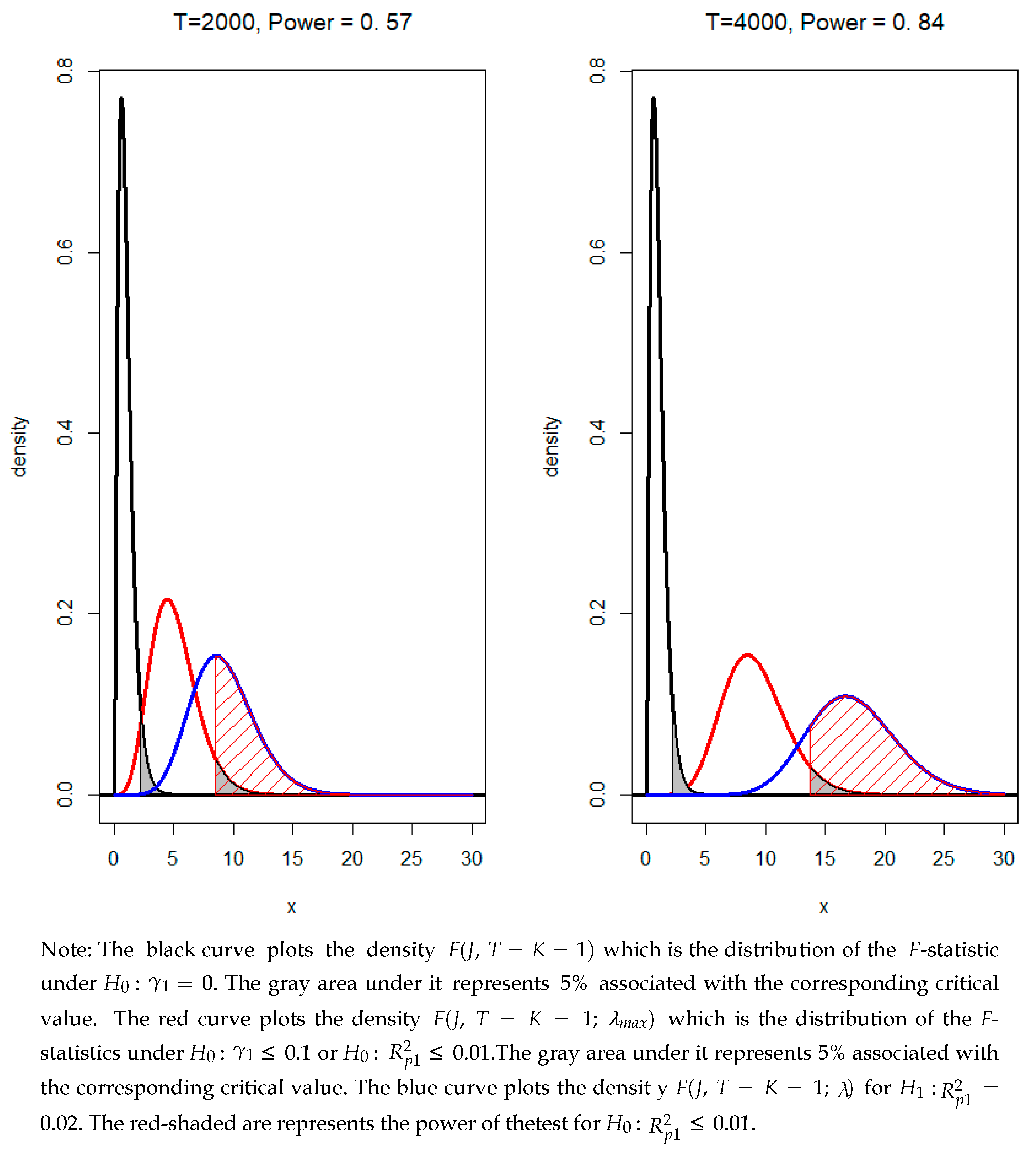
As an illustration, consider a regression where $K=1$. For simplicity, we assume that $Var(X_1)=Var(Y)$, when the sample size T takes values 2000 and 4000. Consider first the case of point-null hypothesis where $H_0:{\gamma }_1=0$. The black curves in Figure 1 plot the density $F(J,T-K-1)$, which is the distribution of the F-statistic under $H_0:{\gamma }_1=0$, for each sample size of 2000 and 4000. It is clear that the 5% critical value does not change with increasing sample size. Since F-statistic is an increasing function of sample size, rejection of $H_0:{\gamma }_1=0$ will eventually occur (except of course for the rare case that the true value of ${\gamma }_1$ is really numerically identical to zero).

Suppose the researcher tests for a minimum effect: $H_0:0\le {\gamma }_1\le 0.1$ against $H_1:{\gamma }_1>0.1$. Since $R_{p1}^2={\gamma }_1^{2}Var(X_1)/Var(Y)$ and $R_{p0}^2=0$, the null and alternative hypotheses can be formulated as $H_0:R_{p1}^2\le 0.01$ against $H_1:R_{p1}^2>0.01$. The red curves in Figure 1 plot the density $F(J,T-K-1;{\lambda }_{max})$ associated with $R_{p1}^2=0.01$ for each sample size. The gray under area under represents 5%, indicated by the critical value which is the 95th percentile of the red curve. It appears that this critical value increases with sample size. The blue curve plots the density $F(J,T-K-1;\lambda )$ associated with $H_1:R_{p1}^2=0.02$ and the red shaded area represents the power of the test for $H_0:R_{p1}^2\le 0.01$. It shows that the power increases with sample size.

It is often the case in economics and finance that a test for linear restrictions is conducted involving a number of regression parameters. For example, under the point-null paradigm, the null hypothesis can be formulated as $H_0:{\gamma }_1={\gamma }_2=0$ for a regression of Y on $X_1$ and $X_2$. In the context of minimum-effect test, the null hypothesis can be written as

$$H_0:({\gamma }_{1l}\le {\gamma }_1\le {\gamma }_{1u})\cup ({\gamma }_{2l}\le {\gamma }_2\le {\gamma }_{2u}),$$

where ${\gamma }_{il}$ and ${\gamma }_{iu}$ for ($i=1,2$) denote the boundaries of economic significance. In this case, the null hypothesis can be formulated in terms of $R_{pj}^2$. That is,

$$H_0:\eta \le {\eta }_{max},$$

where ${\eta }_{max}$ is the maximum population signal-to-noise ratio implied by $R_{pj}^2$. The researcher can formulate the value of $R_{p1}^2-R_{p0}^2$ as the economically significant incremental contribution of ($X_1$, $X_2$) to Y, where the value of $R_{p0}^2$ can be estimated from the regression with restriction ${\gamma }_1={\gamma }_2=0$. Let ${\lambda }_{max}=T{\eta }_{max}$, then if the F-statistic is greater than $F_{\alpha ,{\lambda }_{max}}$, the $\alpha$-level critical value from $F(J,T-K-1;{\lambda }_{max})$, the null hypothesis of the minimum-effect is rejected at the $\alpha$-level of significance. An example in a more general setting can be found in Section 4.1.2.

3.5. Bootstrap Implementation

The tests introduced so far are valid under the assumption of normality. When the assumption of normality is questionable, the one-tailed tests, confidence intervals and the distribution $F(J,T-K-1;\lambda )$ can be implemented using the bootstrap (Efron and Tibshirani 1994). Since there are extensive references available for bootstrapping the p-value and confidence intervals for a one-sample t-test, the details are not given here.

For the minimum-effect test in the linear regression model, the researcher may want to obtain the bootstrap counterpart of the red curve in Figure 1, when the underlying normality is questionable. Consider a simple case of $H_0:0\le {\gamma }_1\le 0.1$ against $H_1:{\gamma }_1>0.1$. Since ${\gamma }_1=0.1$ is associated with the maximum value of $R_{p1}^2$ of 0.01, we consider the regression model under the restriction ${\gamma }_1=0.1$. That is,

$$Y={\widehat{\gamma }}_0+0.1X_1+e,$$

where ${\widehat{\gamma }}_0$ is the estimator for ${\gamma }_0$ under the restriction ${\gamma }_1=0.1$ and e represents the associated residuals. Generate the artificial data $Y^{\ast }$ given $X_1$ as

$$Y^{\ast }={\widehat{\gamma }}_0+0.1X_1+e^{\ast },$$

where $e^{\ast }$ is a random resample of e with replacement. Calculate the F-statistic from $\{Y^{\ast },X_1\}$, denoted as $F^{\ast }$. Repeat the above process sufficiently many times, say B, to obtain ${\{F^{\ast }(i)\}}_{i=1}^B$, which represents the bootstrap distribution for $F(J,T-K-1;\lambda )$.

When a number of parameters are involved with the linear restrictions being tested, the bootstrap can be conducted at the parameter values which maximize the value $\lambda$. As an example, consider the minimum-effect test

$$H_0:({\gamma }_{1l}\le {\gamma }_1\le {\gamma }_{1u})\cup ({\gamma }_{2l}\le {\gamma }_2\le {\gamma }_{2u}).$$

Let ${\widehat{\gamma }}_1$ and ${\widehat{\gamma }}_2$ denote the values under the above $H_0$ which jointly imply the largest economic impact on Y. The bootstrap is conducted with the restrictions ${\gamma }_1={\widehat{\gamma }}_1$ and ${\gamma }_2={\widehat{\gamma }}_2$.

3.6. Model Equivalence Test

Lavergne (2014) proposes a general framework based on the Kullback-Leibler information to assess the approximate validity of multivariate restrictions in parametric models, which is labeled as model equivalence testing. Consider a random sample $X_t$ ($t=1,\dots T$) whose probability density function is denoted as $f(X|{\theta }_0)$ where ${\theta }_0\in \mathsf{\Theta }$ the parameter space. Let $g({\theta }_0)=0$ denote multivariate restrictions on ${\theta }_0$ with r number of restrictions. As a measure of closeness to the true distribution, Lavergne (2014) adopts the Kullback-Leibler information criterion, which is defined as

$$KLIC=E_{{\theta }_0}\left[log\frac{f(X|{\theta }_0)}{f(X|{\theta }_0^c)}\right],$$

where $E_{{\theta }_0}$ denotes the expectation when ${\theta }_0$ is the parameter value and ${\theta }_0^c$ is the value which maximizes $E_{{\theta }_0}logf(X|{\theta }_0)$ under $g({\theta }_0^c)=0$. Noting that $KLIC\ge 0$ and it is 0 when the restriction $g({\theta }_0)=0$ holds exactly, Lavergne (2014) considers the null and alternative hypotheses of the form

$$H_0:2KLIC\ge {\delta }^2/T;H_1:2KLIC<{\delta }^2/T,$$

(7)

where ${\delta }^2\equiv T{\Delta }^2$ while ${\Delta }^2$ being the tolerance of substantive importance. Rejection of $H_0$ implies that the restriction $g({\theta }_0)=0$ is close to be valid.

According to Lavergne (2014), the above model equivalence test can be conducted using the log-likelihood ratio (LR) test, which can be written as

$$LR=2\left[L(\widehat{\theta })-L({\widehat{\theta }}^c)\right],$$

(8)

where $\widehat{\theta }$ denotes the unrestricted (quasi) maximum likelihood estimator for $\theta$ and ${\widehat{\theta }}^c$ the restricted (quasi) maximum likelihood estimator. The LR statistic follows a non-central chi-squared distribution with r degrees of freedom with the non-centrality parameter ${\delta }^2$, denoted as ${\chi }_{r,{\delta }^2}^2$. The null hypothesis is rejected in favor of model equivalence if the LR statistic is less than ${\chi }_{r,{\delta }^2}^2(\alpha )$, which is the $\alpha$th percentile of ${\chi }_{r,{\delta }^2}^2$.

Note that the vanishing tolerance ${\delta }^2/T$ is based on a theoretical consideration, as Lavergne (2014, p. 416) points out. In practical applications, a fixed tolerance ${\Delta }^2$ is chosen so that ${\delta }^2=T{\Delta }^2$. This means that the degree of non-centrality of ${\chi }_{r,{\delta }^2}^2$ increases with sample size, so does the critical value of the test. This is a feature different from the point-null hypothesis testing where the critical value is obtained from a central distribution regardless of sample size. Lavergne (2014) has shown that, in the regression context, $2KLIC$ measures the loss in explanatory power coming from imposing the constraint relative to the error’s variance. Hence, if the researcher sets ${\Delta }^2=0.1$, the models under $H_0$ and $H_1$ are considered to be equivalent if the loss of explanatory power due to imposing the restriction is no more than 10%. Lavergne (2014) provides further asymptotic theories of the test, along with empirical applications.

3.7. Equivalence Test for Model Validation

Model validation or specification tests are often performed based on the paradigm of point null hypothesis testing, for which the null hypothesis is that the model is valid, and the alternative hypothesis is that the model is not valid. Such tests inherit the problems associated with the conventional statistical testing. As Box (1976) points out, all models are wrong, they are approximations to the true data-generation process; consequently a test based on a sharp null hypothesis is not suitable. It is possible that, in small samples, the tests may commit Type II errors due to low power, whereas in large samples all models are found to be rejected due to extreme power (see, for example, Spanos 2017).

As a consequence, Robinson and Froese (2004) recommended the use of equivalence tests for model validation, arguing that using traditional point-null hypothesis testing, as commonly done, enabled the rejection of good models when the data were too many and the failure to reject poor models when the data were too few. Furthermore, equivalence tests permit the expression of a ‘region of equivalence’, within which model predictions could be close enough to reality to be useful, without necessarily being exactly identical (see, e.g., Kleijnen 1995; Robinson 2019). The principle was further extended by Robinson et al. (2005), who produced an equivalence-based variant of a regression-style test originally proposed by Cohen and Cyert (1961). We now summarize Robinson et al.’s (2005) approach.

Assume that we have computer simulation results $x_i$, $i=i,\dots ,n$ that are intended to represent process observations $y_i$. For example, y could be the heights of a sample of trees selected from a forest, and x the predicted heights for the same trees having been computed using the tree diameter and some mathematical function that we wish to validate; $\widehat{y}=x=f(d;\beta )$. Centre the predictions: $x_i^{\ast }=x_i-\overline{x}$. Fit the linear regression model $y_i={\beta }_0+{\beta }_1{x}_i^{\ast }+{ϵ}_i;{ϵ}_i\stackrel{d}{=}N(0,{\sigma }^2)$. Then, perform a TOST on the null hypothesis that ${\beta }_0\ne 0$ as a test of model bias and a TOST on the null hypothesis that ${\beta }_1\ne 1$ as a test of the model fidelity, where fidelity is taken to mean both the spread of the predictions compared to the observations and the order of the predictions compared to the observations. The estimate of the slope will reflect how well the predictions match the spread of the observations—close to 1 is good, and the standard error of the slope will reflect how well the quantiles of the predictions match the quantiles of the observations—small is good. In this way, several interpretable characteristics of model performance can be distilled from the omnibus test. Robinson (2019) provides a more detailed explanation with examples, and Robinson (2016) provides an R (R Core Team 2017) package that runs such tests1.

3.8. Choosing the Limits of Economic Significance

The choice of the limits of economic significance is the most critical step for interval-based tests. Detailed discussions in the contexts of psychology and medical research appear in Murphy and Myors (1999), Walker and Nowacki (2011) and Lakens et al. (2018), among others. These limits affect the outcomes of the test, and also provide scientific credibility to the research outcome. The limits should be determined by the researcher, in consideration of economic theories and meaningful effect size. In so doing, economic reasoning or theory can be incorporated into statistical decision-making.

As Murphy and Myors (1999, p. 237) point out, the choice of limits requires “value judgment”. The choice can also be “context-dependent”, since it may depend on the type of dependent variable involved; and can also depend on the likelihood or seriousness of Type I and II errors. It would be desirable to have a set convention or a consensus of expert opinions in the related field as to the extent of “negligible effects” that could be economically ignored. One may also use meta-analytic evidence from past studies.

The researcher can be guided by estimation-based measures to further justify their choice. For example, one may choose the limits so that they imply the smallest effect size guided by the value of Cohen’s d (Cohen 1977), which is a measure of effect size (the mean difference divided by the standard deviation of the data). In the regression context, the limits may be determined so that the implied economic impact provides a certain value of (incremental) signal-to-noise ratio $\eta$ given in (6) (which is also called Cohen’s $f^2$) or desired coefficient of determination $R_{pj}^2$. For example. if Y is stock return and X is a proposed factor, the interval can be formulated so that X can explain at least 5% of the total variation of stock return ($R_{p1}^2=0.05$; and $R_{p0}^2=0$). This is based on the judgment that an economically meaningful factor should explain at least 5% of the stock return variation, in the absence of other factors. Again, this choice requires value judgment that can be context-dependent. For example, the choice may be different across markets depending on the market conditions such as the trading cost, regulatory framework, and development of market structure, among others. The researcher may consider a number of different values or possible candidates of this value, and make a decision considering the inferential outcomes and their economic significance. However, most ideally, the choice of the limits should be made before the researcher observes the data.

The proposed interval can be indicative of the decision when the point estimate is available. However, the point estimate is subject to sampling variability and it is necessary to conduct the test to make a more informed decision under sampling variability. Proposing such an interval may be equivalent to providing a prior distribution for the Bayesian inference. It is well known that the outcome of the Bayesian inference in large part depends on the choice of prior. But if the choice is made based on concrete economic reasoning and evidence, the Bayesian inference can provide an informed decision. Similarly, if the interval of economic significance is proposed with concrete economic rationale, then it can help the researcher make a correct decision.

Furthermore, it is important for the researcher to include the key components of the test in reporting, such as the interval of equivalence. Doing so serves two purposes: first, it enables the reader to apply different intervals for different applications, and second, it provides a check against unscrupulous researchers choosing intervals that suit their narrative.

4. Empirical Applications

In this section, we provide empirical applications of the interval-based tests discussed in Section 3 to economics and finance. We present two cases where large sample size is used; and one case of a small sample.

4.1. A SAD Stock Market Cycle

In empirical finance, a large number of market anomalies have been identified, where it is claimed that a stock market is systematically influenced by the factors unrelated with the market fundamentals. The evidence is at odds with the efficient market hypothesis which is a cornerstone of modern finance theories. Central to this is the findings that investors’ mood systematically and negatively affects stock return. For example, it is hypothesized that less sunlight or more cloudiness negatively affect investors’ mood, which in turn exerts a negative impact on stock market return. The seminal papers in this area of literature include Saunders (1993), Hirshleifer and Shumway (2003), and Kamstra et al. (2003). However, as Kim (2017) reports, the studies in this area typically show negligible effects with high statistical significance, accompanied by large sample size and negligible $R^2$ values.

Kamstra et al. (2003) study the effect of depression linked with seasonal affective disorder (SAD) on stock return. They claim that, through the link between SAD and depression, and the link between depression and risk aversion, seasonal variation in length of day can translate into seasonal variation in equity return. They consider the regression model of the following form:

$$R_t={\gamma }_0+\sum _{i=1}^2{\gamma }_i{R}_{t-i}+{\gamma }_3{M}_t+{\gamma }_4{T}_t+{\gamma }_{5}SA{D}_t+{\gamma }_6{F}_t+{\gamma }_7{C}_t+{\gamma }_8{P}_t+{\gamma }_9{G}_t+{ϵ}_t,$$

(9)

where $R_t$ denotes the stock return in percentage on day t; M a dummy variable for Monday; T a dummy for the last trading day or the first five trading days of the tax year; F a dummy for fall; C cloud cover, P a precipitation; and G temperature. $SA{D}_t$ is a measure of seasonal depression, which takes the value of $H_t-12$ where $H_t$ represents the time from sunset to sunrise if the day t is in the fall or winter; 0 otherwise.

Kamstra et al. (2003; p. 326) argue that lower returns should commence with autumn because depressed investors shunning risk and re-balance their portfolio in favor of safer assets (i.e., ${\gamma }_6<0$). This is followed by abnormally higher returns when days begin to lengthen and SAD-affected investors begin resuming their risky holdings (i.e., ${\gamma }_5>0$). They use the daily index return data from the markets around the world: U.S. (S&P 500, NYSE, NASGAQ, AMEX), Sweden, U.K., Germany Canada, New Zealand, Japan, Australia, and South Africa. They report, nearly for all markets, that the parameter estimate of ${\gamma }_5$ is positive and statistically significant at a conventional level of significance; and that of ${\gamma }_6$ is negative and statistically significant. These results are the basis of their evidence for the existence of the SAD effects around the world. However, the results are based on the point null hypothesis at a conventional level of significance under large sample sizes, for which Rao and Lovric (2016) among others are concerned about. In this section, we evaluate the regression results of Kamstra et al. (2003) using the interval-based tests.

4.1.1. Evaluating the Results of Kamstra et al.

We first conduct the interval tests using the regression results reported in Kamstra et al. (2003).

Table 1. Testing for the SAD effect.

Market	T	${\mathit{R}}^2$	F	$\mathit{CR}$	${\mathit{CR}}_1$	${\mathit{CR}}_2$	${\mathit{CR}}_3$
US1	18,380	0.011	20.43	1.83	26.87	120.25	245.15
US2	9688	0.027	29.84	1.88	15.76	66.27	133.20
US3	7083	0.033	26.82	1.88	12.33	49.83	99.26
US4	9688	0.091	107.66	1.88	15.77	66.27	133.20
SWE	4836	0.017	9.28	1.88	9.29	35.46	69.70
UK	4534	0.009	4.57	1.88	8.87	33.51	65.69
GER	9411	0.008	8.42	1.88	15.40	64.53	129.61
CAN	8308	0.030	28.52	1.88	13.96	57.58	115.26
NZ	2627	0.010	3.31	1.94	6.79	23.49	45.04
JAP	12,783	0.002	3.20	1.94	22.11	96.18	194.77
AUS	5521	0.010	6.19	1.88	10.22	39.86	78.75
SA	7247	0.010	8.12	1.88	12.54	50.87	101.41

US1: United States, S&P500, from 04 January 1928 to 29 December 2000; US2: United States, NYSE, from 1962-07-05 to 2000-12-29; US3: United States, NASDAQ, from 1972-12-18 to 2000-12-29; SWE: Sweden from 1982-09-15 to 2001-12-18; UK: Britain from 1984-01-04 to 2001-12-06; GER: Germany from 1965-01-05 to 2001-12-12; CAN: Canada from 1969-01-03 to 2001-12-18; NZ: New Zealand from 1991-07-02 to 2001-12-18; JAP: Japan from 1950-04-05 to 2001-12-06; AUS: Australia from 1980-01-03 to 2001-12-18; SA: South Africa from 1973-01-03 to 2001-12-06; T: sample size, calculated using R package “bizdays” (Freitas 2018) from the sample ranges reported in Kamstra et al. (2003; Table 2); $R^2$: $R^2$ values reported in Kamstra et al. (2003; Table 4A–C); F: F-statistic for the joint significance of regression slope coefficients; $CR$: 5% critical values from a central F distribution for $H_0:R^2=0$; $C{R}_1$: 5% critical values for $H_0:0\le R^2\le 0.01$; $C{R}_2$: 5% critical values for $H_0:0\le R^2\le 0.05$; $C{R}_3$: 5% critical values for $H_0:0\le R^2\le 0.10$.

reports the sample size (T) and $R^2$ values of the regression (9), reproduced from Kamstra et al. (2003; Table 2 and 4A–C). From these values, we calculate the F-statistic for joint significance of all slope coefficients are jointly zero ($H_0:{\gamma }_1=\dots ={\gamma }_9=0$), as reported in Table 1. The $CR$ column reports the 5% critical values from the central F distributions, which are around 1.88 regardless of sample size. It appears that the F-test for joint significance is clearly rejected for all markets at a conventional significance level, which indicates that the all slope coefficients of regression (9) are statistically significant. However, this is at odds with negligible $R^2$ values reported in Table 1 which indicate little predictive power for all markets.

Suppose that, for a regression model for stock return to be economically significant, it should explain at least 5% of the return variation. That is, we test for $H_0:0\le R_{p1}^2\le 0.05$ against $H_1:R_{p1}^2>0.05$. The column labeled $C{R}_2$ reports the 5% critical values associated with $F(J,T-K-1;{\lambda }_{max})$ while the value of ${\lambda }_{max}$ is associated with $R_{p1}^2=0.05$ (and $R_{p0}^2=0$). According to these critical values, the null hypothesis of economically negligible effect cannot be rejected for all market indices except for US4. The critical values listed in column $C{R}_1$ are those associated with $H_0:0\le R_{p1}^2\le 0.01$, which delivers rejection in four markets only. If we test for $H_0:0\le R_{p1}^2\le 0.1$, the critical values in column labeled $C{R}_3$ indicate that the predictive power of the estimated models are economically negligible for all markets.

Economic significance of the magnitude of regression coefficients reported in Kamstra et al. (2003) is also questionable. For example, for the U.S. market with S&P500 index (US1), ${\widehat{\gamma }}_6=-0.058$ and its 90% confidence interval is $[-0.10,-0.01]$. The point estimate means that the stock return is on average lower by 0.058% during the autumn period. Suppose, for a factor to have an economically meaningful impact on stock return, its marginal effect should be at least 0.5% (either positive or negative) to justify transaction cost. Then, one can formulate the null hypothesis of economically negligible effect as $H_0:-0.5\le {\gamma }_6\le 0.5$. The 90% confidence interval is clearly within this bound, so we do not reject $H_0$ at the 5% level of significance. The same inferential outcomes apply to all the other regression coefficients of (9) reported in Kamstra et al. (2003). Note that, depending on the attitude of the researcher, one can formulate the null hypothesis as $H_0:({\gamma }_6<-0.5)\cup ({\gamma }_6>0.5)$, but it is also clearly rejected at the 5% level in favor of a negligible effect. Although Kamstra et al. (2003) justify their effect size using the annualized return, this annualized return does not take account of the underlying volatility of stock return or trading costs involved.

4.1.2. Replicating the Results of Kamstra et al.

We now replicate the model (9) using the value-weighted daily returns from the NYSE composite index (CRSP). The SAD variable and other dummy variables are generated following Kamstra et al. (2003), using programming language R (R Core Team 2017). The data for weather variables (C, P, and G) are collected from the National Center for Environmental Information.2 Our data for the regression ranges from January 1965 to April 1996 (7886 observations), due to the limited availability of the weather data (C) for New York. We have the following estimated values for the key coefficients: ${\widehat{\gamma }}_5=0.032$ with t-statistic of 2.29; ${\widehat{\gamma }}_6=-0.055$ with t-statistic of $-2.17$; and $R^2=0.05$. These values are fairly close to those reported in Table 4A of Kamstra et al. (2003).

We first pay attention to the point null hypothesis that $H_0:{\gamma }_5={\gamma }_6=0$ for joint significance of the SAD effects. The F-statistic is 3.18 with the p-value of 0.04, rejecting $H_0$ at the 5% significance level. This is despite the observation that the incremental contribution of these two variables is negligible, measured by $R_1^2-R_0^2=0.0008$ with $R_1^2=0.0501$ and $R_0^2=0.0493$. Next, we consider an interval hypothesis of minimum-effect. Suppose that the incremental contribution of these variables should be at least 0.01 to be economically significant. That is,

$$H_0:(R_{p1}^2-R_{p0}^2)\le 0.01.$$

Assuming $R_{p0}^2=0.05$, ${\lambda }_{max}=83.87$ and the corresponding 5% critical value is 58.97, obtained from $F(J,T-K-1;{\lambda }_{max})$. With this critical value being much larger than the F-statistic of 3.18, the above interval null hypothesis of minimum-effect cannot be rejected at the 5% level, providing evidence that the SAD economic cycle is economically negligible in the U.S. stock market.

4.2. Empirical Validity of an Asset-Pricing Model

An asset-pricing model explains the variation of asset return as a function of a range of risk factors. The most fundamental is the capital asset pricing model (CAPM) which stipulates that an asset (excess) return is a linear function of market (excess) return. The slope coefficient (often called beta) measures the sensitivity of an asset return to the market risk. While the CAPM is theoretically motivated, the market risk alone cannot fully explain the variation of asset return. In response to this, several multi-factor models have been proposed, which augment the CAPM with a number of empirically motivated risk factors such as the size premium or value premium (see, for example, Fama and French 1993). The most recently proposed multi-factor model is the five-factor model of Fama and French (2015), which can be written as

$$R_{it}-R_{ft}=a_i+b_i(R_{Mt}-R_{ft})+s_{i}SM{B}_t+h_{i}HM{L}_t+r_{i}RM{W}_t+c_{i}CM{A}_t+e_{it},$$

(10)

where $R_{it}$ is the return on an asset or portfolio i at time t ($i=1,\dots ,N;t=1,\dots ,T)$, $R_{ft}$ is the risk-free rate, $R_{Mt}$ is the return on a (value-weighted) market portfolio at time t, $SM{B}_t$ is the return on a diversified portfolio of small stocks minus the return on a diversified portfolio of big stocks, the $HM{L}_t$ is the spread in returns between diversified portfolios of high book-to-market stocks and low book-to-market stocks, $RM{W}_t$ is the spread in returns between diversified portfolios of stocks with robust and weak profitability, and the $CM{A}_t$ is the spread in returns between diversified portfolios of low and high investment firms. The precursors to this 5-factor model include the 3-factor model of Fama and French (1993) which include $(R_{Mt}-R_{ft})$, $SMB$, and $HML$; and the 4-factor model of Carhart (1997) which adds momentum factor ($MOM$) to the 3-factor model. If these factors fully or adequately capture the variation of asset return, then the intercept terms $a_i$ (which may be may be interpreted as the risk-adjusted return) should be zero or sufficiently close to it. On this basis, the model’s empirical validity is evaluated by testing for $H_0:a_1=\dots =a_N=0$, which is a point-null hypothesis.

4.2.1. GRS Test: Minimum-Effect

The F-test for $H_0$ is widely called the GRS test, proposed by Gibbons et al. (1989). Let $a={(a_1,\dots ,a_N)}^{\prime }$ be the vector of N intercept terms, and $\mathsf{\Sigma }$ be the $N\times N$ covariance matrix of error terms. The model (10) is estimated using the ordinary least-squares: $\widehat{a}$ denotes the estimator for a and $\widehat{\mathsf{\Sigma }}$ the estimator for $\mathsf{\Sigma }$. The F-test statistic is written as

$$F=\frac{T(T-N-K)}{N(T-K-1)}\frac{{\widehat{a}}^{\prime }{\widehat{\mathsf{\Sigma }}}^{-1}\widehat{a}}{1+{\widehat{\mu }}^{\prime }{\widehat{\mathsf{\Omega }}}^{-1}\widehat{\mu }},$$

(11)

where T is the sample size, $K=5$ is the number of risk factors, $\widehat{\mathsf{\Omega }}$ is the $K\times K$ covariance matrix of risk factors, and $\widehat{\mu }$ is the $K\times 1$ mean vector. Under the assumption that the error terms e’s follow a multivariate normal distribution, the statistic follows the $F(N,T-N-K;\lambda )$ distribution, with the non-centrality parameter

$$\lambda =\left(\frac{T}{1+{\widehat{\theta }}^2}\right)a^{\prime }{\mathsf{\Sigma }}^{-1}a=\left(\frac{T}{1+{\widehat{\theta }}^2}\right)({\theta }^{\ast 2}-{\theta }^2),$$

(12)

where $\widehat{\theta }$ is the ex-post maximum Sharpe ratio of K-factor portfolio, $\theta$ is the ex-ante maximum Sharpe ratio of K-factor portfolio, and ${\theta }^{\ast }$ is the slope of the ex ante efficient frontier based on all assets. Gibbons et al. (1989) call $\theta /{\theta }^{\ast }$ the proportion of the potential efficiency. Note that, under $H_0$, this ratio is equal to one and $\lambda =0$.

However, perfect efficiency cannot exist in practice. It is unrealistic that all of a values are jointly and exactly zero. On this point, it is sensible to consider an interval-based hypothesis testing. For example, consider $H_0:0.75<\theta /{\theta }^{\ast }\le 1$ against $H_1:\theta /{\theta }^{\ast }<0.75$. This is on the basis of judgment that the factors with the proportion of potential efficiency of 0.75 or higher provide practically efficient asset-pricing.

The data is available from French’s data library monthly from 1963 to 2015 ($T=630$).3 We use 25 portfolio returns ($N=25$) sorted by size and book-to-market ratio extensively analyzed by Fama and French (1993, 2015).

Table 2. GRS test for asset-pricing models.

Model	GRS	${\mathit{R}}^2$	$\left|\mathit{a}\right|$	$\mathit{CR}$	${\mathit{CR}}_1$	Ratio
CAPM	4.41	0.74	0.25	1.52	1.88	0.25
3-factor	3.61	0.92	0.10	1.52	2.62	0.46
4-factor	3.07	0.92	0.09	1.52	3.70	0.63
5-factor	2.79	0.92	0.09	1.52	4.03	0.67

CAPM: the model with single factor $(R_{Mt}-R_{ft})$; 3-factor: CAPM plus $SMB$ and $HML$ (Fama and French 1993); 4-factor: 3-factor plus $MOM$ (Carhart 1997); 5-factor: 3 factor plus $RMW$ and $CMA$ (Fama and French 1993); GRS: GRS test statistic $H_0:a_1=\dots =a_N=0$; $R^2$: average $R^2$ values over $N=25$ equations; $\left|a\right|$: average intercept estimates over $N=25$ equations; CR: 5% critical value from $F(N,T-N-K)$; $C{R}_1$: 5% critical value from $F(N,T-N-K,{\lambda }_{max})$; ratio: sample estimate of $\theta /{\theta }^{\ast }$.

reports the test results. The GRS test for $H_0:a_1=\dots =a_N=0$ are clearly rejected for all models considered, with the p-value (not reported) practically 0 for all cases. The critical values of this test (from the central F distributions) is listed in the column labeled $CR$. This results suggest that none of the asset pricing models are able to fully capture asset return variations. This is at odds with the high values of $R^2$ and small values of $\left|a\right|$, especially multi-factor models. For the 4-factor and 5-factor model, the estimated ratio of potential efficiency is much higher than other models, close to 0.7.

Table 2 also reports the critical values ($C{R}_2$) for $H_0:0.75<\theta /{\theta }^{\ast }\le 1$, which is calculated from $F(N,T-N-K,{\lambda }_{max})$ distribution with the value of ${\lambda }_{max}$ implied by $\theta /{\theta }^{\ast }=0.75$. It is found that, for the 4-factor and 5-factor models, $H_0:0.75<\theta /{\theta }^{\ast }\le 1$ cannot be rejected at the 5% level of significance. This suggests that these multi-factor model have captured the variation of asset returns adequately, with economically negligible deviation from the perfect efficiency. For the CAPM and 3-factor models, the interval-based $H_0$ is rejected at the 5% level, but this seems consistent with the estimated values of potential efficiency which are less than 0.5 for both cases. It is worth noting that the critical values $CR$ for the point-null hypothesis (based on the central F-distribution) are nearly identical for all cases, regardless of the estimation results such as $R^2$ and $\left|a\right|$. However, those for the interval-based tests are different, depending on the model estimation results.

4.2.2. LR Test: Model Equivalence

We now test for the validity of the asset-pricing models using the model equivalence test discussed in Section 3.6. We calculate the LR test for given in (8) for $H_0:a_1=\dots =a_N=0$, which is written as

$$LR=T(log\{det[\widehat{\mathsf{\Sigma }}(H_0)]\}-log\{det[\widehat{\mathsf{\Sigma }}(H_1)]\}),$$

where $\widehat{\mathsf{\Sigma }}(H_i)$ denotes the maximum likelihood estimator for $\mathsf{\Sigma }$ under $H_i$. For the model equivalence test given in (7), the above LR statistic follows the ${\chi }_{N,{\delta }^2}^2$ distribution with ${\delta }^2=T{\Delta }^2$. Using the same data set as in Section 4.2.1, the LR statistic is 105.67, 88.05, 75.82, and 69.26 for the CAPM, 3-factor model, 4-factor model, and 5-factor model respectively. If we set ${\Delta }^2$ to 0.1, the 5% critical value is 61.12, indicating that $H_0$ is not approximately valid for all models. If we set ${\Delta }^2$ to 0.15, the 5% critical value is 87.19, indicating $H_0$ is approximately valid only for 4-factor and 5-factor models. If we set ${\Delta }^2$ to 0.20, the 5% critical value is 114.00, indicating that $H_0$ is approximately valid for all models. It appears that the results are sensitive to the choice of ${\Delta }^2$ values. However, at a reasonable value of ${\Delta }^2=0.15$, the results are consistent with the minimum-effect test based on the GRS test conducted above.

4.3. Testing for Persistence of a Time Series

The presence of a unit root in economic and financial time series has strong implications to many economic theories and their empirical validity (see Choi 2015). For example, a unit root in the real exchange rate is evidence that the purchasing power parity does not hold (Lothian and Taylor 1996); and a unit root in the real GNP supports the view that a shock to the economy has a permanent effect, which is not consistent with the traditional (or Keynesian) view of business cycle (Campbell and Mankiw 1987). To test for the hypothesis, the unit root test proposed by Dickey and Fuller (1979) has been widely used, while a large number of its extensions and improvement have been proposed. The augmented Dickey–Fuller (ADF) test for a time series Y is based on the regression of the form

$$\Delta Y_t={\delta }_0+{\delta }_{1}t+\theta Y_{t-1}+\sum _{j=1}^{m-1}{\rho }_j\Delta Y_{t-j}+u_t,$$

(13)

where $\Delta Y_t=Y_t-Y_{t-1}$; m is the autoregressive (AR) order of Y; and $u_t$ is an $i.i.d.$ error term with zero mean and fixed variance. Note that $\theta \equiv \tau -1$ where $\tau$ is the sum of all AR(m) coefficients in level of Y, measuring the degree of persistence. The test for a unit root is based on point-null hypothesis of $H_0:\theta =0$ against $H_1:\theta <0$. Under $H_0$, the t-test statistic asymptotically follows the Dickey–Fuller distribution, from which the critical values of the test are obtained. Under $H_1$, the t-test statistic asymptotically follows the standard normal distribution.

The problems of the unit root test are well documented (see, for example, Choi 2015). The most well-known is its low power (at a conventional significance level), which means that there is a high chance of committing Type II error (failure to reject a false null hypothesis). On this point, Kim and Choi (2017) propose the unit root test at the optimal level of significance, which is obtained by minimizing the expected loss from hypothesis testing. They find that the optimal level is in the 0.3 and 0.4 range for many economic time series, arguing that the exclusive use of 0.05 level has led to accumulation of false stylized facts. The other problem of the test is the discontinuity of the sampling distributions of the test statistic under $H_0$ and $H_1$. This makes the decision highly sensitive to the value specified under $H_0$.

More importantly, as discussed in Section 2.3, it is unrealistic to assume that an economic time series such as the real GNP or real exchange rate has an autoregressive root exactly equal to one. An economist may wish to test whether a time series shows a degree of persistence practically different from that of a unit root time series. The test can be conducted in the context of non-inferiority test discussed in the previous section. To do this, we need to find the value of $\tau$ or $\theta$ under which a time series shows a practically different degree of persistence from a unit root time series. According to DeJong et al. (1992), a plausible value of $\tau$ under $H_1:\theta <0$ is 0.85, 0.95, 0.99 for annual, quarterly and monthly data respectively, which translate to the $\theta$ values of $-0.15$, $-0.05$, and $-0.01$. On this basis, we test for the persistence of a time series using the following interval hypotheses:

$$H_0:\theta \le {\theta }_1;H_1:\theta >{\theta }_1,$$

where ${\theta }_1\in \{-0.15,-0.05,-0.01\}$ depending on the data frequency. The time series is practically trend-stationary under this $H_0$. This test is a standard one-sample t-test whose statistic asymptotically follows the standard normal distribution. However, we note that the least-squares estimator for $\tau$ or $\theta$ is biased in small samples, which may adversely affect the small sample properties of the test. As an alternative to the non-inferiority test, we also use the bias-corrected bootstrap confidence interval for $\theta$ for improved statistical inference, similar to those of Kilian (1998a, 1998b) and Kim (2004).

For a set of time series $(Y_1,\dots .Y_T)$, we first estimate the parameters of model (13) using the bias-corrected estimators. Let $({\widehat{\delta }}_0,{\widehat{\delta }}_1,\widehat{\theta },{\widehat{\rho }}_1,\dots ,{\widehat{\rho }}_{m-1})$ be the bias-corrected estimators; and let $\{e_t\}$ denote the corresponding residual. Generate the artificial data set as

$$Y_t^{\ast }={\widehat{\delta }}_0+{\widehat{\delta }}_{1}t+{\widehat{\beta }}_1{Y}_{t-1}+\dots +{\widehat{\beta }}_m{Y}_{t-m}+e_t^{\ast },$$

using $(Y_1,\dots ,Y_m)$ as the starting values, where $e_t^{\ast }$ is a random draw with replacement from ${\{e_t\}}_{t=m+1}^T$ and $({\widehat{\beta }}_1,\dots ,{\widehat{\beta }}_m)$ are the AR coefficients in level associated with $(\widehat{\theta },{\widehat{\rho }}_1,\dots ,{\widehat{\rho }}_{m-1})$. Using ${\{Y_t^{\ast }\}}_{t=1}^T$, estimate the $AR(m)$ coefficients, again with bias correction, $({\widehat{\delta }}_0^{\ast },{\widehat{\delta }}_1^{\ast },{\widehat{\beta }}_1^{\ast },\dots ,{\widehat{\beta }}_m^{\ast })$. For bias correction, we use Shaman and Stine (1988) asymptotic formula with stationarity-correction, following Kilian (1998b) and Kim (2004). We obtain ${\widehat{\theta }}^{\ast }={\widehat{\tau }}^{\ast }-1$, where ${\widehat{\tau }}^{\ast }={\sum }_{j=1}^m{\widehat{\beta }}_j^{\ast }$. Repeat this process B times to obtain the bootstrap distribution ${\{{\widehat{\theta }}^{\ast }(j)\}}_{j=1}^B$, which can be used as an approximation to the sampling distribution of $\widehat{\theta }$. If the confidence interval for $\theta$ obtained from ${\{{\widehat{\theta }}^{\ast }(j)\}}_{j=1}^B$ covers ${\theta }_1$, then this is evidence that the time series shows a degree of of persistence practically no different from that of a trend-stationary time series.

Table 3. Test for persistence: Extended Nelson–Plosser Data.

	T	p-Value	$\widehat{\mathit{\theta }}$	t-Stat	${\mathit{CI}}_1$	${\mathit{CI}}_2$
R.GNP	80	0.05	−0.140	−0.66	−0.298	−0.037
N.GNP	80	0.58	−0.010	2.96	−0.147	−0.0001
P.GNP	80	0.04	−0.150	−0.82	−0.304	−0.043
IP	129	0.26	−0.098	−0.21	−0.274	−0.002
Emp	99	0.18	−0.118	−0.21	−0.242	−0.031
Uemp	99	0.01	−0.214	−1.53	−0.430	−0.074
Def	100	0.70	−0.003	5.56	−0.081	−0.0001
CPI	129	0.91	−0.002	13.22	−0.019	−0.0001
Wages	89	0.53	−0.026	2.81	−0.144	−0.0002
Rwages	89	0.75	−0.010	1.90	−0.183	−0.0002
MS	100	0.18	−0.037	3.83	−0.110	−0.0016
Vel	120	0.78	−0.001	4.65	−0.099	−0.0001
Rate	89	0.98	−0.025	2.35	−0.191	−0.0004
S&P	118	0.64	−0.021	2.15	−0.144	−0.0002

R.GNP: Real GNP; N.GNP: Nominal GNP: P.GNP: Real per capita GNP; IP” Industrial Production; Emp: Employment; Uemp: Unemployment Rate; Def: GNP deflator; CPI: Consumer Price Index; Wages: Wages; Rwages: Real Wages: MS: Money Stock; Vel: Velocity; Rate: Interest rate; S&P: Common Stock Price. T: Sample size; p-value: p-value of the ADF test for $H_0:\theta =0$; $\widehat{\theta }$: bias-corrected estimators for $\theta$; t-stat: t-statistic for $H_0:\theta \le -0.15$ against $H_1:\theta >-0.15$ based on Equation (13) with 5% critical value of 1.645; $(C{I}_1,C{I}_2)$: lower and upper bounds of 95% bootstrap bias-corrected confidence interval for $\theta$; The AR orders used are same as those of Nelson and Plosser (1982).

reports the results from the extended Nelson and Plosser (1982) data for a set of annual U.S. macroeconomic time series, setting ${\theta }_1=-0.15$. Firstly, the ADF test (a point-null hypothesis test) provides the p-values larger than 0.05 for most of time series, providing evidence that many macroeconomic time series have a unit root. In contrast, the t-test (non-inferiority test) results for $H_0:\theta \le -0.15$ against $H_1:\theta >-0.15$ show that we clearly cannot reject this $H_0$ at the 5% level of significance (asymptotic critical value 1.645) for the real GNP, real per capita GNP, industrial production, employment, unemployment rate, providing evidence that these time series are practically trend-stationary. As for the bootstrap inference, it is found that the 95% bias-corrected bootstrap confidence interval for $\theta$ does cover $-0.15$, for the real GNP, real per capita GNP, industrial production, employment, unemployment rate, real wage, and interest rate, indicating that these time series show the degree of persistence practically of a trend-stationary time series. The two alternative methods are in agreement in their inferential outcomes, except for real wage and interest rate.

The results for the test of persistence based on the non-inferiority test are largely consistent with those of Kim and Choi (2017) who re-evaluate the ADF test results at the optimal level of significance and report evidence that the real GNP, real per capita GNP, employment, and money stock do not have a unit root. These results are also largely consistent with the Bayesian evidence of Schotman and van Dijk (1991).

5. Conclusions

This paper provides a review of interval-based hypothesis testing methods, which are known under the name of minimum-effect, non-inferiority, and equivalence tests in biostatistics and psychology. Although the first proposal of such a test goes back to Hodges and Lehmann (1954), it has attracted little attention in the business disciplines of science. In the latter, the paradigm of point-null hypothesis has been the major workforce in making statistical decisions and establishing research findings. However, as a number of authors have criticized for many years, the current paradigm has a range of limitations and deficiencies, as discussed in Section 2 of this paper. These problems have become even more apparent in the big data era, where the p-value criterion widely and routinely adopted by statistical researchers is no longer usable in making sensible statistical decisions. The consequences are serious, with widespread practice of data-mining (Black 1993), data-snooping (Lo and MacKinlay 1990), p-hacking (Harvey 2017), and multiple testing (Harvey et al. 2016), which result in an embarrassing number of false positives as Harvey (2017) puts it. The related empirical evidence is provided by meta-analytic studies conducted by Kim and Ji (2015) and Kim et al. (2018). Even more serious is systematic distortion of published results, such as publication bias (Basu and Park 2014) and replication crisis (Peng 2015). In light of these problems, Rao and Lovric (2016) call for a new paradigm to be in place for statistical testing in the 21st century, with a proposal of interval-based hypothesis testing as a possible solution.

An important point in favor of adopting an interval-based test is the fact that an economic hypothesis cannot be formulated as a point. Rather, it is more sensible when it takes a form of an interval or a neighborhood: see, for example, De Long and Lang (1992), Leamer (1988), and Startz (2014). For example, when a researcher tests for stock market efficiency, she is not testing for a perfect efficiency (as described by a point-null hypothesis), since such a perfect relationship cannot hold economically (Grossman and Stiglitz 1980). More realistically, the researcher is interested in whether the degree of market inefficiency (Campbell et al. 1997) is economically large enough to be concerned (an interval hypothesis). Hence, it makes more sense to consider an interval hypothesis for decision-making in economic or business research.

As we have seen in this paper, an interval-hypothesis can be implemented in a simple and straightforward manner, using the existing instruments of hypothesis testing such as one-tailed test, confidence interval, and non-central distributions. Its main attraction is that the critical values of these tests increase with sample size, overcoming a major deficiency of point-null hypothesis testing. A key requirement of the test is that the researcher should specify an interval of economic significance under the null or alternative hypothesis, preferably before she observes the data. This may require a value judgment depending on contexts, accompanied by a thorough economic analysis on the effect size of the relationship under investigation. This is an integral part of interval-based hypothesis testing, since it has a strong impact on the test outcome and research integrity. It is also highly desirable that the relevant research community establishes a consensus on the range of minimum effect size that matters economically.

We have applied the interval-based tests to economics and finance applications. The first is a test for market efficiency, whether investors’ mood has a systematic effect on stock market return. While the effect may appear to show statistical significance under the current point-null paradigm, the minimum-effect tests cannot reject its negligible economic effect. The second is on the empirical validity of asset-pricing models. In contrast to the findings based on point-null hypothesis testing, we find that a class of multi-factor models are empirically valid based on minimum-effect and model equivalence tests. The third is on the degree of persistence of economic time series. A unit root test based on a conventional point-null hypothesis strongly favors the presence of a unit root in many macroeconomic time series such as the real GNP. According to the non-inferiority test, many time series in Nelson–Plosser data set are found to show a degree of persistence of a trend-stationary time series, especially in the real income variables. From these applications, we find that the interval-based tests are applicable to many contentious research problems in the business disciplines of science, shedding new lights on the existing results or stylized facts. We propose that interval-based hypothesis tests be widely adopted in business research, especially in the new era of big data.

References

- Arrow, Kenneth. 1960. Decision theory and the choice of a level of significance for the t-test. In Contributions to Probability and Statistics: Essays in Honor of Harold Hotelling. Edited by Ingram Olkin. Stanford: Stanford University Press, pp. 70–78. [Google Scholar]
- Basu, Sudipta, and Han-Up Park. 2014. Publication Bias in Recent Empirical Accounting Research, Working Paper. Available online: http://ssrn.com/abstract=2379889 (accessed on 31 May 2018).
- Berger, James O., and Thomas Sellke. 1987. Testing a Point Null Hypothesis: The Irreconcilability of p-Values and Evidence. Journal of the American Statistical Association 82: 112–22. [Google Scholar] [CrossRef]
- Black, Fischer. 1993. Beta and return. The Journal of Portfolio Management 20: 8–18. [Google Scholar] [CrossRef]
- Box, George E. P. 1976. Science and Statistics. Journal of the American Statistical Association 71: 791–99. [Google Scholar] [CrossRef]
- Campbell, John Y., and N. Gregory Mankiw. 1987. Are Output Fluctuations Transitory? Quarterly Journal of Economics 102: 857–80. [Google Scholar] [CrossRef]
- Campbell, John Y., Andrew W. Lo, and Archie Craig MacKinlay. 1997. The Econometrics of Financial Markets. Princeton: Princeton University Press. [Google Scholar]
- Carhart, Mark M. 1997. On persistence in mutual fund performance. Journal of Finance 52: 57–82. [Google Scholar] [CrossRef]
- Choi, In. 2015. Almost All about Unit Roots. New York: Cambridge University Press. [Google Scholar]
- Cohen, Jacob. 1977. Statistical Power Analysis for the Behavioral Sciences, 2nd ed. New York: LBA. [Google Scholar]
- Cohen, Kalman J., and Richard M. Cyert. 1961. Computer Models in Dynamic Economics. The Quarterly Journal of Economics 75: 112–27. [Google Scholar] [CrossRef]
- De Long, J. Bradford, and Kevin Lang. 1992. Are All Economic Hypotheses False? Journal of Political Economy 100: 1257–72. [Google Scholar] [CrossRef]
- DeJong, David N., John C. Nankervis, N. E. Savin, and Charles H. Whiteman. 1992. Integration versus trend stationary in time series. Econometrica 60: 423–33. [Google Scholar] [CrossRef]
- Dickey, David A., and Wayne A. Fuller. 1979. Distribution of the estimators for autoregressive time series with a unit root. Journal of the American Statistical Association 74: 427–31. [Google Scholar]
- Efron, Bradley, and Robert J. Tibshirani. 1994. An Introduction to the Bootstrap. Boca Raton: Chapman & Hall, CRC Monographs on Statistics & Applied Probability. [Google Scholar]
- Fama, Eugene F., and Kenneth R. French. 1993. Common risk factors in the returns on stocks and bonds. Journal of Financial Economics 33: 3–56. [Google Scholar] [CrossRef] [Green Version]
- Fama, Eugene F., and Kenneth R. French. 2015. A five-factor asset-pricing model. Journal of Financial Economics 116: 1–22. [Google Scholar] [CrossRef]
- Freitas, Wilson. 2018. Bizdays: Business Days Calculations and Utilities. R Package Version 1.0.6. Available online: https://CRAN.R-project.org/package=bizdays (accessed on 31 May 2018).
- Gibbons, Michael R., Stephen A. Ross, and Jay Shanken. 1989. A test of the efficiency of a given portfolio. Econometrica 57: 1121–52. [Google Scholar] [CrossRef]
- Gigerenzer, Gerd. 2004. Mindless statistics: Comment on “Size Matters”. Journal of Socio-Economics 33: 587–606. [Google Scholar] [CrossRef]
- Grossman, Sanford J., and Joseph E. Stiglitz. 1980. On the impossibility of informationally efficient markets. The American Economic Review 70: 393–408. [Google Scholar]
- Harvey, Campbell R. 2017. Presidential Address: The Scientific Outlook in Financial Economics. Journal of Finance 72: 1399–440. [Google Scholar] [CrossRef]
- Harvey, Campbell R., Yan Lin, and Heqing Zhu. 2016. … and the cross-section of expected returns. Review of Financial Studies 29: 5–68. [Google Scholar] [CrossRef]
- Hirshleifer, David, and Tyler Shumway. 2003. Good day sunshine: Stock returns and the weather. Journal of Finance 58: 1009–32. [Google Scholar] [CrossRef]
- Hodges, J. L., Jr., and E. L. Lehmann. 1954. Testing the Approximate Validity of Statistical Hypotheses. Journal of the Royal Statistical Society, Series B (Methodological) 16: 261–68. [Google Scholar] [CrossRef]
- Johnstone, D. J., and D. V. Lindley. 1995. Bayesian Inference Given Data Significant at Level α: Tests of Point Hypotheses. Theory and Decision 38: 51–60. [Google Scholar] [CrossRef]
- Kamstra, Mark J., Lisa A. Kramer, and Maurice D. Levi. 2003. Winter blues: A sad stock market cycle. American Economic Review 93: 324–43. [Google Scholar] [CrossRef]
- Kandel, Shmuel., and Robert F. Stambaugh. 1996. On the Predictability of Stock Returns: An Asset-Allocation Perspective. The Journal of Finance 51: 385–424. [Google Scholar] [CrossRef] [Green Version]
- Keuzenkamp, Hugo A., and Jan Magnus. 1995. On tests and significance in econometrics. Journal of Econometrics 67: 103–28. [Google Scholar] [CrossRef]
- Kilian, Lutz. 1998a. Small sample confidence intervals for impulse response functions. The Review of Economics and Statistics 80: 218–30. [Google Scholar] [CrossRef]
- Kilian, Lutz. 1998b. Accounting for lag-order uncertainty in autoregressions: The endogenous lag order bootstrap algorithm. Journal of Time Series Analysis 19: 531–38. [Google Scholar] [CrossRef]
- Kim, Jae H. 2004. Bootstrap Prediction Intervals for Autoregression using Asymptotically Mean-Unbiased Parameter Estimators. International Journal of Forecasting 20: 85–97. [Google Scholar] [CrossRef]
- Kim, Jae H. 2017. Stock Returns and Investors’ Mood: Good Day Sunshine or Spurious Correlation? International Review of Financial Analysis 52: 94–103. [Google Scholar] [CrossRef]
- Kim, Jae H. 2019. Tackling False Positives in Business Research: A Statistical Toolbox with Applications. Journal of Economic Surveys. [Google Scholar] [CrossRef]
- Kim, Jae H., and In Choi. 2017. Unit Roots in Economic and Financial Time Series: A Re-evaluation at the Decision-based Significance Levels. Econometrics 5: 41. [Google Scholar] [CrossRef]
- Kim, Jae H., and In Choi. 2019. Choosing the Level of Significance: A Decision-Theoretic Approach. Abacus: A Journal of Accounting, Finance and Business Studies. forthcoming. [Google Scholar]
- Kim, Jae H., and Philip Inyeob Ji. 2015. Significance Testing in Empirical Finance: A Critical Review and Assessment. Journal of Empirical Finance 34: 1–14. [Google Scholar] [CrossRef]
- Kim, Jae. H., Kamran Ahmed, and Philip Inyeob Ji. 2018. Significance Testing in Accounting Research: A Critical Evaluation based on Evidence. Abacus: A Journal of Accounting, Finance and Business Studies 54: 524–46. [Google Scholar] [CrossRef]
- Kleijnen, Jack P. C. 1995. Verification and validation of simulation models. European Journal of Operational Research 82: 145–62. [Google Scholar] [CrossRef]
- Labes, Detlew, Helmut Schuetz, and Benjamin Lang. 2018. Power and Sample Size Based on Two One-Sided t-Tests (TOST) for (Bio)Equivalence Studies, R Package Version: 1.4-7. Available online: https://cran.r-project.org/web/packages/PowerTOST/index.html (accessed on 31 May 2018).
- Lakens, Daniel, Anne M. Scheel, and Peder M. Isager. 2018. Equivalence Testing for Psychological Research: A Tutorial. Advances in Methods and Practices in Psychological Science 1: 259–69. [Google Scholar] [CrossRef]
- Lavergne, Pascal. 2014. Model Equivalence Tests in a Parametric Framework. Journal of Econometrics 178: 414–25. [Google Scholar] [CrossRef]
- Leamer, Edward. 1978. Specification Searches: Ad Hoc Inference with Nonexperimental Data. New York: Wiley. [Google Scholar]
- Leamer, Edward. 1988. Things that bother me. Economic Record 64: 331–35. [Google Scholar] [CrossRef]
- Lehmann, Erich L., and Joseph P. Romano. 2005. Testing Statistical Hypotheses, 3rd ed. New York: Springer. [Google Scholar]
- Lo, Andrew W., and A. Craig MacKinlay. 1990. Data Snooping in Tests of Financial Asset Pricing Models. Review of Financial Studies 10: 431–67. [Google Scholar] [CrossRef]
- Lothian, James R., and Mark P. Taylor. 1996. Real exchange rate behavior: The recent float from the perspective of the past two centuries. Journal of Political Economy 104: 488–510. [Google Scholar] [CrossRef]
- McCloskey, Deirdre N., and Stephen T. Ziliak. 1996. The standard error of regressions. Journal of Economic Literature 34: 97–114. [Google Scholar]
- Murphy, Kevin R., and Brett Myors. 1999. Testing the Hypothesis That Treatments Have Negligible Effects: Minimum-Effect Tests in the General Linear Model. Journal of Applied Psychology 84: 234–48. [Google Scholar] [CrossRef]
- Murphy, Kevin R., Brett Myors, and Allen Wolach. 2014. Statistical Power Analysis: A Simple and General Model for Traditional and Modern Hypothesis Tests, 4th ed. New York: Routledge. [Google Scholar]
- Nelson, Charles R., and Charles R. Plosser. 1982. Trends and random walks in macroeconomic time series. Journal of Monetary Economics 10: 139–62. [Google Scholar] [CrossRef]
- Ohlson, James A. 2018. Researchers’ Data Analysis Choices: An Excess of False Positives? Available online: https://ssrn.com/abstract=3089571 (accessed on 31 May 2018).
- Open Science Collaboration. 2015. Estimating the reproducibility of psychological science. Science 349: 6251. [Google Scholar] [CrossRef]
- Peng, Roger. 2015. The Reproducibility Crisis in Science: A Statistical Counterattack. Significance 12: 30–32. [Google Scholar] [CrossRef]
- Peracchi, Franco. 2001. Econometrics. New York: Wiley. [Google Scholar]
- R Core Team. 2017. R: A Language and Environment for Statistical Computing. Vienna: R Foundation for Statistical Computing, Available online: https://www.R-project.org/ (accessed on 31 May 2018).
- Rao, Calyampudi Radhakrishna, and Miodrag M. Lovric. 2016. Testing Point Null Hypothesis of a Normal Mean and the Truth: 21st Century Perspective. Journal of Modern Applied Statistical Methods 15: 2–21. [Google Scholar] [CrossRef] [Green Version]
- Robinson, Andrew P. 2016. Equivalence: Provides Tests and Graphics for Assessing Tests of Equivalence. R Package Version 0.7.2. Available online: https://cran.r-project.org/web/packages/equivalence/index.html (accessed on 31 May 2018).
- Robinson, Andrew P. 2019. Testing Simulation Models Using Frequentist Statistics. In Computer Simulation Validation: Fundamental Concepts, Methodological Frameworks, and Philosophical Perspectives. Edited by Claus Beisbart and Nicole Saam. Berlin: Springer. [Google Scholar]
- Robinson, Andrew P., and Robert E. Froese. 2004. Model validation using equivalence tests. Ecological Modelling 176: 349–58. [Google Scholar] [CrossRef]
- Robinson, Andrew P., Remko A. Duursma, and John D. Marshall. 2005. A regression-based equivalence test for model validation: Shifting the burden of proof. Tree Physiology 25: 903–13. [Google Scholar] [CrossRef] [PubMed]
- Saunders, Edward M. 1993. Stock prices and wall street weather. American Economic Review 83: 1337–45. [Google Scholar]
- Schotman, Peter C., and Herman K. van Dijk. 1991. On Bayesian routes to unit roots. Journal of Applied Econometrics 6: 387–401. [Google Scholar] [CrossRef] [Green Version]
- Shaman, Paul, and Robert A. Stine. 1988. The bias of autoregressive coefficient estimators. Journal of the American Statistical Association 83: 842–48. [Google Scholar] [CrossRef]
- Spanos, Aris. 2017. Mis-specification testing in retrospect. Journal of Economic Surveys 32: 541–77. [Google Scholar] [CrossRef]
- Startz, Richard. 2014. Choosing the More Likely Hypothesis. Foundations and Trends in Econometrics 7: 119–89. [Google Scholar] [CrossRef]
- van der Laan, Mark, Jiann-Ping Hsu, Karl E. Peace, and Sherri Rose. 2010. Statistics ready for a revolution: Next generation of statisticians must build tools for massive data sets. Amstat News 399: 38–39. [Google Scholar]
- Walker, Esteban, and Amy S. Nowacki. 2011. Understanding Equivalence and Noninferiority Testing. Journal of General Internal Medicine 26: 192–96. [Google Scholar] [CrossRef] [PubMed]
- Wasserstein, Ronald L., and Nicole A. Lazar. 2016. The ASA’s statement on p-values: Context, process, and purpose. The American Statistician 70: 129–33. [Google Scholar] [CrossRef]
- Wellek, Stefan. 2010. Testing Statistical Hypotheses of Equivalence and Noninferiority, 2nd ed. New York: CRC Press. [Google Scholar]
- Wellek, Stefan, and Peter Ziegler. 2017. EQUIVNONINF: Testing for Equivalence and Noninferiority. R Package Version 1.0. Available online: https://CRAN.R-project.org/package=EQUIVNONINF (accessed on 31 May 2018).
- Winer, Ben J. 1962. Statistical Principles in Experimental Design. New York: McGraw-Hill. [Google Scholar]
- Ziliak, Steve T., and Deirdre Nansen McCloskey. 2008. The Cult of Statistical Significance: How the Standard Error Costs Us Jobs, Justice, and Lives. Ann Arbor: The University of Michigan Press. [Google Scholar]