Forecasting Industrial Production Using Its Aggregated and Disaggregated Series or a Combination of Both: Evidence from One Emerging Market Economy

Abstract

In this paper, we address whether using a disaggregated series or combining an aggregated and disaggregated series improves the forecasting of the aggregated series compared to using the aggregated series alone. We used econometric techniques, such as the weighted lag adaptive least absolute shrinkage and selection operator, and Exponential Triple Smoothing (ETS), as well as the Autometrics algorithm to forecast industrial production in Brazil one to twelve months ahead. This is the novelty of the work, as is the use of the average multi-horizon Superior Predictive Ability (aSPA) and uniform multi-horizon Superior Predictive Ability (uSPA) tests, used to select the best forecasting model by combining different horizons. Our sample covers the period from January 2002 to February 2020. The disaggregated ETS has a better forecast performance when forecasting horizons that are more than one month ahead using the mean square error, and the aggregated ETS has better forecasting ability for horizons equal to 1 and 2. The aggregated ETS forecast does not contain information that is useful for forecasting industrial production in Brazil beyond the information already found in the disaggregated ETS forecast between two and twelve months ahead.

1. Introduction

Economic agents make decisions based on their views on the present state of the economy and their expectations for the future. The general levels of output, employment, interest rates, exchange rates, and inflation are key economic indicators that help to diagnose a country’s economic situation. Therefore, the proposition and evaluation concerning the ability of econometric models to forecast a country’s economic reality introduce benefits that create better guides for economic agents and policymakers.

One of the main macroeconomic indicators of an economy is the gross domestic product (GDP), which is a proxy for a country’s economic performance. We use industrial production as a proxy for the GDP since the monthly industrial production index is of higher frequency than the GDP. Moreover, the industrial production index is released with a lag of one month, which is smaller than that of the GDP, which has a delayed release of more than two months.

We address whether using a disaggregated series or combining an aggregated and disaggregated series improves the forecasting accuracy of the aggregated series compared to using the aggregated series alone for the industrial production in Brazil series. Disaggregated data refer to the decomposition of the main variable into several sub-components, which have different weights for the aggregated series. We obtained a forecast of these sub-components individually and then we grouped the forecasts of these sub-components to estimate the forecast of the aggregated series. This alternative could increase the accuracy of the forecast; we modeled the sub-components by taking their characteristics into account. We used this alternative in the present work to understand if there was a reduction in the forecast error of the aggregate series by estimating a model for each sub-component.

The literature addresses the accuracy of using disaggregated or aggregated data for forecasting. According to Lütkepohl (1987), the forecast using disaggregation is theoretically optimal if the disaggregated series is uncorrelated; the author suggests using disaggregation if the correlation between the disaggregated series is not strong. Some examples of contributions to the theoretical literature on aggregate or disaggregate forecasting include Lütkepohl (1984, 1987); Granger (1987); Pesaran et al. (1989); Van Garderen et al. (2000); and Giacomini and Granger (2004). The following questions arise: Does aggregating a disaggregated forecast improve the accuracy of the aggregate forecast? One alternative is to estimate using only the lagged aggregate variable to forecast the aggregate series. Giacomini (2015) points out that the results of the empirical literature are mixed, but that disaggregation can improve the forecast accuracy of the aggregate variable. Another alternative is to combine the disaggregate and aggregate series and select the relevant variables to forecast the aggregate series. Hendry and Hubrich (2011) suggest this as a promising direction when using model selection procedures, even though the authors developed a dynamic factor model to consider the disaggregation and did not develop a selection procedure.

Our goal was to determine whether forecasting the disaggregated components of industrial production in Brazil or combining these components with the aggregate series, improve the forecast accuracy of Brazil’s aggregate industrial production compared to using only the lagged aggregate variable. We analyzed Brazil as the 9th GDP in dollars based on 2019 World Bank data. In addition, Brazil is an emerging economy, so it has a more volatile business cycle than advanced countries, a stylized fact in the literature as seen in Aguiar and Gopinath (2007), and in Kohn et al. (2021), among others. This higher volatility can lead to difficulty in forecasting Brazilian economic activity, another motivator for our research.

We do not know of any other articles that address the contributions of disaggregated data from the weighted lag adaptive least absolute shrinkage and selection operator (WLadaLASSO) methodology or from exponential triple smoothing (ETS), selecting the most appropriate model or the relevant variables from the combination of a disaggregate and aggregate series to forecast industrial production. Only Bulligan et al. (2010) analyzed the contributions of disaggregated data to forecast industrial production, and we intend to fill this gap. The topic of disaggregation or aggregation in forecasting is most commonly studied for the inflation and GDP series, such as Espasa et al. (2002); Marcellino et al. (2003); Hubrich (2005); Carlo and Marçal (2016); and Heinisch and Scheufele (2018). Additionally, we analyzed the forecast accuracies of the models based on the multi-horizon superior predictive ability method developed by Quaedvlieg (2021) by combining different horizons, which is different from other forecast comparison procedures that focus on the model performances of the models for each horizon separately. Quaedvlieg (2021) developed the average multi-horizon superior predictive ability (aSPA) and uniform multi-horizon superior predictive ability (uSPA) tests to compare a multi-horizon forecast. Using monthly data from January 2002 to February 2020, we selected the best model for a rolling window of 100 fixed observations and evaluated the forecast for industrial production in Brazil one to twelve months ahead. We used 91 rolling windows. We considered the first-order autoregressive model (AR(1)), AR(1) with time-varying parameters (TVP-AR(1)), the thirteenth-order autoregressive model (AR(13)), and the unobserved components with stochastic volatility (UC-SV) estimated based on Barnett et al. (2014) as naive models. We also analyzed the following methods for selecting the best model: ETS based on Hyndman et al. (2002, 2008) and Hyndman and Khandakar (2008), the least absolute shrinkage and selection operator (LASSO), adaptive LASSO (adaLASSO), the WLadaLASSO, and the Autometrics algorithm. We used the LASSO and its variants to select the lags from the fifteenth-order autoregressive model (AR(15)). Additionally, we considered the Autometrics algorithm that selects the lags from an AR(15) and the dummy variables for outliers or breaks in the sample. In addition, we combined the disaggregated and aggregated series in the model to forecast the general industrial production. To reduce the dimensionality of this model with the combination, we adopted the LASSO and adaLASSO procedures, and the Autometrics algorithm. We compared the forecasting performance between the models based on the mean square error (MSE), the modified Diebold and Mariano (1995) test (henceforth, the MDM test), the model confidence set (MCS) procedure from Hansen et al. (2011), the forecast encompassing test from Harvey et al. (1998), and the multi-horizon superior predictive ability from Quaedvlieg (2021).

Our MSE results point to the ETS model having a better forecasting accuracy for industrial production in Brazil compared to other models. The disaggregated ETS model is the ETS model for each disaggregated series. The disaggregated ETS model leads to the lowest MSE among all of the models for all the forecast horizons, except for those that are one and two months ahead. For the forecasts that are one and two months ahead, the aggregate ETS model has a lower MSE, and there is little difference compared to the disaggregated ETS model. The aggregated ETS model is the ETS model using the lagged aggregated series as covariates. The disaggregated ETS model also has a lower MSE than the forecast of the combination of the aggregated and disaggregated series. This result is similar to that of Faust and Wright (2013), who determined that the combination of the disaggregated and aggregated series does not lead to a better forecast compared to aggregating the disaggregated forecasts; however, their study focused on the United States (US) consumer price index (CPI). Our results are in the opposite direction of the results by Hendry and Hubrich (2011) and Weber and Zika (2016). To analyze whether there was better statistical performance, we used the ETS with disaggregated data as a benchmark in the MDM test. The disaggregated ETS model presents a better forecast performance compared to the naive models (AR(1), AR(13), TVP-AR(1), UC-SV), LASSO, and variants, and the Autometrics algorithm, considering aggregated and disaggregated data (or a combination of both). Only the aggregated ETS model has equal predictive accuracy to the disaggregated ETS model for the forecast horizons of one to five, seven, ten, and twelve months ahead based on the MDM test. The set of “best” models for the most forecast horizons includes only the disaggregated and aggregated ETS models with 90% probability according to the MCS. In 2 of the 12 forecasting horizons, the MCS only has the disaggregated ETS model. We also used the forecast encompassing test. Results showed that the optimal combination forecast only incorporated forecasts from the disaggregated ETS model and the aggregated ETS model. The disaggregated ETS forecast was the only model to be considered in the optimal combination forecast of industrial production for 10 horizons among the 12 analyzed, comparable to the aggregated ETS model. Aggregated ETS does not contain information that is useful for forecasting industrial production in Brazil beyond the information already found in the disaggregated ETS between two and twelve months ahead. When we analyzed the 12 horizons together, we rejected the null hypothesis of equal predictability for all of the models compared to the disaggregated ETS by the uSPA and aSPA tests at 5% statistical significance. In short, we determined that the ETS model presents the best forecast performance comparatively, which is a result similar to that of Elliott and Timmermann (2008). The disaggregated ETS is superior after 6 horizons when compared to the aggregated ETS based on the aSPA test. The aggregated ETS only introduces relevant information to forecast industrial production for one period ahead compared to the disaggregated ETS according to the forecast encompassing test, which indicates the superiority of disaggregated information for industrial production, which is in line with Bulligan et al. (2010).

This article contains five sections in addition to this introduction. Section 2 reviews the literature. Next, we will address the methodologies of the models considered in the paper in Section 3. Section 4 presents our data, the empirical forecasting strategy, the MDM test, the MCS procedure, the forecast encompassing test, and the aSPA and uSPA tests to compare how the models perform. In Section 5, we will analyze the results of the study. Finally, Section 6 presents the concluding remarks.

2. Literature Review

This section discusses the differences in the forecast accuracy in three scenarios—aggregating the disaggregated forecasts, only modeling the aggregate variable, and combining the aggregated and disaggregated series. Bulligan et al. (2010) analyzed the forecasting performance of industrial production models in Italy with forecast horizons that ranged from 1 to 3 months ahead. They determined that disaggregated models have better forecast performance based on the root of MSE. There are not many analyses in the literature that differentiate between the use of the disaggregated and aggregated series to forecast the aggregated series of industrial production. As such, we have to fill in this gap.

Carstensen et al. (2011) compared the ability of indicators to forecast industrial production in the Euro area. The authors were unable to determine any indicator that was dominant as the best predictor of the industrial production because it depends on the forecast horizon and the loss function considered. Additionally, the forecast of the AR(1) model is quite difficult to beat during quiet times based on the fluctuation test by Giacomini and Rossi (2010). Rossi and Sekhposyan (2010) found that the useful predictors for forecasting US industrial production change over time. However, they did not use a disaggregated series of industrial production as Carstensen et al. (2011) did. Kotchoni et al. (2019) analyzed the performance of models selecting factors from 134 monthly macroeconomic and financial indicators to forecast industrial production, and they compared these models to standard time series models. They found that the MCS selected the LASSO model for forecasting during periods of recessions, but did not choose it to forecast the full out-of-sample data.

When addressing the forecast ability of other economic variables, Marcellino et al. (2003) found evidence that the individual estimation of inflation in each Euro area country and the subsequent aggregation of projections increase the forecast accuracy related to forecasting of this variable at the aggregate level. Hubrich (2005) determined that aggregating the forecasts of each component of inflation does not necessarily better predict inflation in the Euro area one year ahead. Espasa et al. (2002) had similar results, indicating that disaggregation leads to better projections for periods longer than one month. Carlo and Marçal (2016) compared forecasts from models for aggregate inflation and those aggregating the forecasts for the components from the Brazilian inflation index. The authors determined that the forecast using disaggregated data increased accuracy, such as Heinisch and Scheufele (2018).

Zellner and Tobias (2000) studied the effects of aggregated and disaggregated models in forecasting the average annual GDP growth rate of 18 countries. In general, disaggregation led to more observations that could be used to estimate the parameters, but the authors obtained better predictions for the aggregate variable. Barhoumi et al. (2010) analyzed the forecasting performance of France’s GDP between alternative factor models. They wanted to know whether it was more appropriate to extract factors from aggregate or disaggregated data for forecasting purposes. Rather than using 140 disaggregated series, Barhoumi et al. (2010) showed that the static approach of Stock and Watson (2002) using 20 aggregate series led to better prediction results. In other words, the mentioned articles present favorable evidence for the use of a disaggregated series or to model using an aggregated series only, leaving the question open.

Hendry and Hubrich (2011) proposed an alternative use of a disaggregate variable to forecast the aggregate variable, which was a combination of disaggregated and aggregated variables. This is different from previous literature, which suggested forecasting the disaggregate variables and then aggregating them to obtain the forecast of the aggregate variable, as we discussed earlier in this section. Hendry and Hubrich (2011) determined that including disaggregate variables in the aggregate model improves the forecast accuracy if the disaggregates have different stochastic structures and if the components are interdependent, according to Monte Carlo simulations. They sought to forecast US inflation by considering the sectorial breakdown of inflation. To reduce the dimension of the disaggregate variables, they used the factor model with the results of using this combination, corroborating those obtained by the Monte Carlo simulations. Hendry and Hubrich (2011) introduced (as a promising direction for procedures) selection of the disaggregated series and their lags together with the lags of the aggregate series to predict the aggregate series.

Faust and Wright (2013) analyzed the forecasting models for the US CPI. They considered the combination idea from Hendry and Hubrich (2011) and compared the use of the aggregated or disaggregated series individually in the model, but did not suggest procedures for variable selection. They determined that the combination model did not lead to a better forecasting performance for the aggregated series according to the root of the MSE when compared to disaggregated or aggregated models. Weber and Zika (2016) sought to forecast general employment in Germany as a function of its lags and disaggregation in different sectors. However, the authors used principal components to summarize information from the sectors. They determined that the disaggregation improved the forecast for general employment when compared to the univariate model for the aggregate series. As such, the contributions of this article include the results of combining the aggregated and disaggregated series and using the variable selection procedure to fill this gap.

Regarding the literature on the methodologies used in this work, Epprecht et al. (2021) conducted a Monte Carlo simulation experiment that considered the data generating process (DGP) to be a linear regression with orthogonal variables and independent data. The authors determined that adaLASSO and the Autometrics algorithms also have similar forecasting performances when there are a small number of relevant variables and when the number of candidate variables is lower than the number of observations. The Autometrics algorithm only performs better when it has a large number of relevant variables (as 15 to 20) because of the bias against the penalization term in adaLASSO. Additionally, Epprecht et al. (2021) determined that adaLASSO performs better than LASSO and the Autometrics algorithm for linear regression with orthogonal variables in terms of model performance. Autometrics is only preferable with small samples. The authors also used genomics data to compare the predictive power to the epidermal thickness in psoriatic patients, in which covariates are not orthogonal. Out-of-sample forecasts with variables that were selected via LASSO, adaLASSO, or Autometrics cannot be statistically differentiated by the MDM test.

Kock and Teräsvirta (2014) used a neural network model with three algorithms to model monthly industrial production and unemployment series from the Group of Seven (G7) countries and Denmark, Finland, Norway, and Sweden. They focused on forecasting during the economic crisis from 2007 to 2009. The authors found that the Autometrics algorithm performs worse with direct forecasts than with recursive forecasts because the model is not a reasonable approximation of reality (as it excludes the most relevant lags).1 The Autometrics algorithm tends to select a highly parameterized model that does not present competitive forecasts compared to other methodologies in direct forecasting. That is, Kock and Teräsvirta (2014) determined that the Autometrics algorithm may perform worse when there are considerable misspecifications in the general model. In the present work, we used recursive forecasting, in which, according to Kock and Teräsvirta (2014), the Autometrics algorithm does not perform badly. The next section presents the methodology used in this paper.

3. Methodology

We considered four naive models to compare our forecasts: UC-SV and an autoregressive model with constant parameters or with time-varying parameters. Our goal was to select the lagging variables that were relevant based on different univariate methodologies. We used LASSO and two of its variants (adaLASSO and WLadaLASSO), the exponential smoothing method, and the Autometrics algorithm. We used the variable $\mathsf{\Delta }{y}_t$ in the cases of AR(1), AR(13), TVP-AR(1), LASSO and its variants, and the Autometrics algorithm because the series $y_t$ is non-stationary and $\mathsf{\Delta }{y}_t$ removes a unit root from the dynamics, where $\mathsf{\Delta }$ is the first difference operator.2 In the case of UC-SV and exponential smoothing, we used the variable $y_t$.

3.1. Time-Varying Parameters Autoregressive Model of First Order

In this section, we present the methodology of the TVP-AR(1) model. We used this model to obtain a naive forecast and only considered one lag in the model. The methodology using time-varying parameters seeks to contemplate the changes that can occur in the economy over time (Kapetanios et al. 2019). Considering the TVP-AR(1) model, the measurement equation can be written as

$$\mathsf{\Delta }{y}_t={\beta }_{0t}+{\beta }_{1t}\mathsf{\Delta }{y}_{t-1}+{\epsilon }_t$$

(1)

where ${\epsilon }_t\sim N\left(0,{\sigma }^2\right)$ for $t=1,...,T$, and $\mathsf{\Delta }{y}_0$ is an initial observation. We can write the autoregressive and the constant coefficients ${\beta }_t={\left({\beta }_{0t},{\beta }_{1t}\right)}^{\top }$ with the following transition equation

$${\beta }_t={\beta }_{t-1}+u_t$$

(2)

where $u_t\sim N\left(0,\mathsf{\Omega }\right)$, ⊤ is the transpose of a matrix and the transition equation has the initial value ${\beta }_1\sim N\left({\beta }_0,{\mathsf{\Omega }}_0\right)$.

We used the Bayesian estimation according to Kroese et al. (2014). See Appendix A.1 for more details. Next, we will explain the UC-SV model that we used in the present study.

3.2. UC with Stochastic Volatility

Stock and Watson (2007) included stochastic volatility in an unobserved component model. The authors showed that UC-SV performed well when forecasting US inflation. The UC-SV model is defined as

$$y_t={\beta }_t+{\sigma }_t^{\frac{1}{2}}{v}_t$$

(3)

$${\beta }_t={\beta }_{t-1}+{\omega }_t^{\frac{1}{2}}{e}_t$$

(4)

where $ln{\sigma }_t$ and $ln{\omega }_t$ are the logarithm of the stochastic volatility, ${\beta }_t$ is the trend, $ln{\sigma }_t=ln{\sigma }_{t-1}+e_{1t}$, and $ln{\omega }_t=ln{\omega }_{t-1}+e_{2t}$. We allowed the variances of $e_{1t}$ and $e_{2t}$ to be distinct following Barnett et al. (2014), which is different from Stock and Watson (2007) who assumed that the variances of the two stochastic volatility processes were equal.3 The variances of $e_{1t}$ and $e_{2t}$ are denoted by $g_1$ and $g_2$, respectively.4

We estimated the model using the Markov chain Monte Carlo (MCMC) method with the Gibbs sampling method following Barnett et al. (2014). We describe the MCMC method in Appendix A.2, and we detail the Bayesian estimation and the priors in Appendix A.3.

3.3. LASSO-Type Penalties

In this subsection, we present three lasso-type penalties to select the relevant lags for the univariate model from an AR(15): LASSO, adaLASSO, and WLadaLASSO.

3.3.1. LASSO

Tibshirani (1996) proposed the LASSO method based on the following minimization problem

$${\widehat{\beta }}^{LASSO}=argmi{n}_{{\beta }_0,{\beta }_1,...,{\beta }_k}{\displaystyle \sum _{t=1}^T}{\left(\mathsf{\Delta }{y}_t-{\beta }_0-\sum _{j=1}^k{\beta }_j\mathsf{\Delta }{y}_{t-j}\right)}^2+\lambda {\displaystyle \sum _{j=1}^k}\left|{\beta }_j\right|$$

(5)

where $\lambda \ge 0$ is a tuning parameter. LASSO needs a value for $\lambda$, which we will explain shortly. The first term is the sum of the square of the residuals and the second term is a shrinkage penalty. ${\displaystyle \sum _{j=1}^k}\left|{\beta }_j\right|$ is the ${\ell }^1$ norm of a coefficient vector $\beta$. The ${\ell }^1$ penalty forces some of the coefficient estimates to be equal to zero when $\lambda$ is sufficiently large. As such, the LASSO technique can perform the variable selection.

Cross-validation is usually the method choice for obtaining $\lambda$ value. With the time series data, we used the Bayesian information criterion (BIC) to choose $\lambda$ according to Konzen and Ziegelmann (2016), based on a grid of $\lambda$ values. The grid of possible values for $\lambda$ is $\left(0,0.5,1,...,10\right)$.

3.3.2. AdaLASSO

Zou (2006) stated that LASSO can lead to the inconsistent selection of variables that maintain noisy variables for a given $\lambda$. Additionally, the author showed that LASSO could lead to correct variable selections using biased estimates for large coefficients, resulting in suboptimal prediction rates.

As such, Zou (2006) introduced adaLASSO, which considers weights ${\omega }_j$ that adjust the penalty to be different for each coefficient. The adaLASSO seeks to minimize

$${\widehat{\beta }}^{adaLASSO}=argmi{n}_{{\beta }_0,{\beta }_1,...,{\beta }_k}{\displaystyle \sum _{t=1}^T}{\left(\mathsf{\Delta }{y}_t-{\beta }_0-\sum _{j=1}^k{\beta }_j\mathsf{\Delta }{y}_{t-j}\right)}^2+\lambda {\displaystyle \sum _{j=1}^k{\omega }_j}\left|{\beta }_j\right|$$

(6)

where ${\omega }_j=\mid {\widehat{\beta }}_j^{ridge}\mid {}^{-\tau }$, $\tau >0$. adaLASSO considers that large (small) coefficients have small (large) weights and small (large) penalties. We used ridge regression estimated coefficients ${\widehat{\beta }}^{ridge}$ to determine the weight ${\omega }_j$. Ridge regression shrinks the vectors of the coefficients by penalizing the sum of the squares of the residuals:

$${\widehat{\beta }}^{ridge}=argmi{n}_{{\beta }_0,{\beta }_1,...,{\beta }_k}{\displaystyle \sum _{t=1}^T}{\left(\mathsf{\Delta }{y}_t-{\beta }_0-\sum _{j=1}^k{\beta }_j\mathsf{\Delta }{y}_{t-j}\right)}^2+\lambda {\displaystyle \sum _{j=1}^k}{\beta }_j^2$$

(7)

where the penalty is the ${\ell }^2$ norm of the $\beta$ vector. Ridge regression is not a variable selection method because this regression obtains non-zero estimates for all coefficients.

3.3.3. WLadaLASSO

When we used adaLASSO with the time series data, each coefficient was associated with a lagged variable and penalized according to the size of the ridge regression’s estimate. The less distant the lag in the variable, the more important the variable must be for the model; therefore, its coefficient should be penalized less (considering the case without seasonality).

Park and Sakaori (2013) proposed different types of penalties for different lags. Konzen and Ziegelmann (2016) denominated the adaLASSO with weighted lags based on those from Park and Sakaori (2013) as WLadaLASSO. The WLadaLASSO method is calculated as:

$${\widehat{\beta }}^{wladaLASSO}=argmi{n}_{{\beta }_0,{\beta }_1,...,{\beta }_k}{\displaystyle \sum _{t=1}^T}{\left(\mathsf{\Delta }{y}_t-{\beta }_0-\sum _{j=1}^k{\beta }_j\mathsf{\Delta }{y}_{t-j}\right)}^2+\lambda {\displaystyle \sum _{j=1}^k{\omega }_j^w}\left|{\beta }_j\right|$$

(8)

where ${\omega }_j^w={\left(\mid {\widehat{\beta }}_j^{ridge}\mid e^{-\alpha l}\right)}^{-\tau }$ is the weight, $\tau >0$, $\alpha \ge 0$, l is the order of the variable’s lag, and e is the exponential function. We set the parameter $\tau$ equal to one for adaLASSO and WLadaLASSO, which was the case in Konzen and Ziegelmann (2016). We considered a grid for $\alpha$, where the set of possible values for $\alpha$ was $\left(0,0.5,1,...,10\right)$. We calculated the optimal $\lambda$ among those possible for that model with the lowest BIC value for each $\alpha$ value. We chose the $\alpha$ value from the model producing the smallest BIC value among all of the possible $\alpha$ values, following Konzen and Ziegelmann (2016).

3.4. Exponential Smoothing

The name exponential smoothing comes from the idea that recent observations are more important to forecasting than older observations and, therefore, have a greater weight to forecast. Exponential smoothing is basically an exponentially weighted sum of past values (to obtain the forecast). We can represent the ETS method as a state space model (Hyndman et al. 2002, 2005; Ord et al. 1997).

We can decompose the economic series into certain components, such as trends (T), cycles (C), seasonality (S), and irregularities or error (E). We used the ETS method to decompose the series into these components. Only the cycle component was not decomposed separately so that it could be modeled along with the trend component following Hyndman and Khandakar (2008) and Hyndman et al. (2008). Thus, we can combine the trend, seasonality, and error components.

Hyndman and Khandakar (2008) and Hyndman et al. (2008) proposed 15 different combinations among the trend and seasonality components. The trend represents the long-term direction of the series. The trend component presents five different possibilities: none, additive, additive damped, multiplicative, and multiplicative damped. The trend component is a combination of the level $\left(\ell \right)$ and growth $\left(b\right)$ parameters. $T_h$ is the forecast trend over the next h periods, and $\varphi$ is a damping parameter $\left(0<\varphi <1\right)$. As such, if there is no trend component, $T_h=\ell$. If the trend component is additive, $T_h=\ell +bh$. If the trend component is additively damped, $T_h=\ell +\left(\varphi +{\varphi }^2+\cdots +{\varphi }^h\right)b$. If the trend component is multiplicative, $T_h=\ell b^h$. If the trend component is multiplicative damped, $T_h=\ell b^{\left(\varphi +{\varphi }^2+\cdots +{\varphi }^h\right)}$. If the growth rate at the end of the series is unlikely to continue, then the damped trend seems to be the most reasonable option.

The next step is to detail the types of seasonal components. There are three types of seasonal components: none, additive, and multiplicative. Additionally, the error component can be additive or multiplicative, but this distinction is not relevant for point forecasting (Hyndman et al. 2008).

As such, we considered the combination of five types of trend components and three types of seasonal components, resulting in 15 types of ETS models, following Hyndman and Khandakar (2008). These 15 possibilities are presented in Table 1 of Hyndman et al. (2008), in which the first entry refers to the trend component and the second refers to the seasonal component.

Basically, the estimation procedure is based on estimating the smoothing parameters and the initial state variables maximizing the likelihood function. The algorithm proposed by Hyndman et al. (2002) also determines which of the 15 ETS models is the most appropriate by selecting the model based on the information criterion. The information criteria used to select the most appropriate model are AIC corrected for small sample bias (AICc), as suggested by Talagala et al. (2018). See Appendix A.4 for more details. We present the Autometrics algorithm in the next subsection.

3.5. Autometrics Algorithm

We used the Autometrics algorithm (Castle et al. 2011; Doornik 2008) to address potential instability points and structural changes and to select the lags of the dependent variable that were relevant. The algorithm is based on an approach called the London School of Economics econometric methodology, in which the specification search starts from the GEneral model, and using specification and misspecification tests, the model can be simplified To a Specific model, called GETS. From a general unrestricted model, the algorithm attempts to reduce the unrestricted model through combinations of variables in the general model to evaluate the relevance of these variables to eliminate the irrelevant variables (variables with coefficients that are statistically insignificant). During each step, attempting to reduce the model, the algorithm performs diagnostic tests on the errors to verify the congruence of the models after variables are eliminated.5 The purpose of this procedure is to determine the most comprehensive and parsimonious model that is a good representation of the local DGP.

The Autometrics algorithm starts by using a general model in which there are up to 15 lags in the dependent variable for industrial production in Brazil using the following equation

$$\mathsf{\Delta }{y}_t=\sum _{i=1}^{15}{\rho }_i\mathsf{\Delta }{y}_{t-i}+\sum _{l=1}^T\left({\alpha }_{l}II{S}_l\right)+\sum _{s=1}^{11}{\theta }_{s}S{e}_s+{\epsilon }_t$$

(9)

where $II{S}_l$ is an impulse variable that is only equal to one at $t=l$ and zero otherwise (Pretis et al. 2018). $S{e}_s$ is the monthly dummy variable for each month s. ${\epsilon }_t$ is the error term.

There are two types of models that use Autometrics. The first is the “without outlier” type, which does not consider any type of outlier in the general model. The second type is the “IIS” type, which allows the dummy variables to control for the outlier in the specific model. See Appendix A.5 for more details.

3.6. Combination of Aggregated and Disaggregated Series

Hendry and Hubrich (2011) proposed combining a disaggregated and aggregated series to forecast the aggregated series because it could improve the forecast accuracy. However, we considered the combination of the two using the variable selection procedure from the following general model:

$$\mathsf{\Delta }{y}_{g,t}=\sum _{i=1}^{15}\left({\rho }_i\mathsf{\Delta }{y}_{g,t-i}\right)+\sum _{i=0}^{15}\sum _{j=1}^{24}\left({\beta }_{ji}\mathsf{\Delta }{y}_{j,t-i}\right)+{\epsilon }_t$$

(10)

where $y_{g,t}$ is the general industrial production; $y_{j,t-i}$ is the industrial production of sector j and includes a total of 24 sectors—the disaggregated series.

We had 399 parameters—disregarding the constant—to estimate this equation, which was greater than the number of observations for each rolling window—100 observations (defined in Section 4.1). As such, we needed to reduce the dimensionality. We used three methods to select the relevant variables and their lags: LASSO, adaLASSO, and the Autometrics algorithm. Thus, we considered three different methodologies for combining the disaggregated and aggregated series to forecast the general industrial production.

However, we needed the forecast of the disaggregated series to obtain the forecast for the general industry for h months ahead. For this, we used the forecasts for the disaggregated series that we estimated with each univariate model discussed earlier: the AR(1), TVP-AR(1), UC-SV, ETS; LASSO and its variants; and the Autometrics algorithm and its variant. As such, we had three procedures to select the relevant variables for Equation (10); for each procedure, we used the forecasts for each sector using the 11 models to estimate the forecast for the general industrial production. In this sense, we analyzed 33 different possible combinations. Once again, we used the significance level $\alpha =0.1\%$ in the Autometrics algorithm for the combinations.

4. Data and Empirical Strategy

Our data were the logarithm of the industrial production in Brazil index at the general level and its disaggregation by sectors. The data were from the Monthly Industrial Survey of Physical Production (PIM-PF) from the Brazilian Institute of Geography and Statistics (IBGE). We used monthly data from January 2002 to February 2020 and did not make any seasonal adjustments. We did not consider vintage data or past revisions for these series. We removed a unit root from the dynamics using the first difference of the series, with the exception of the UC-SV and ETS models.

The general industry forecast was carried out using a model that only included the lags in this series; we compared this forecast to the forecast for each sector (aggregated according to weight) to obtain the general industry forecast. We used the weights for each sector according to PIM-PF. According to the IBGE, the weights for each sector have been fixed since 2002, which is our period of analysis.

In addition, we compared the forecast of the aggregate model with the combination of the aggregated and disaggregated series. Thus, we used disaggregated data for the extractive industry and for the 25 sectors of the manufacturing industry. However, two sectors, “printing and reproduction of recordings”, and “maintenance, repair and installation of machines and equipment”, only presented data from January 2012 and, therefore, we did not include these sectors in the estimates.6 Thus, our disaggregated sample includes the extractive industry category and 23 sectors of the manufacturing industry.

We present the behavior of the logarithm concerning general industrial production in Brazil between January 2002 and February 2020 in Figure 1. There is evidence of seasonality in the series. In addition, the series had an increasing growth rate between 2002 and 2008; between 2009 and 2014 there was no growth in the series. Between 2014 and 2016 there was a fall in industrial production—a period that is noted as being a recession according to the official Brazilian committee for dating business cycles (CODACE).7 There has been no growth in the series since 2017.

Table A1. Descriptive statistics in the first difference ($\mathsf{\Delta }{y}_t$) and ${\mathsf{\Delta }}_{12}{y}_t$.

	$\mathsf{\Delta }{\mathit{y}}_{\mathit{t}}$	${\mathsf{\Delta }}_{12}{\mathit{y}}_{\mathit{t}}$
Mean	0.0002	0.0023
Standard deviation	0.0283	0.0281
Maximum	0.0722	0.0754
Minimum	−0.0850	−0.0808
First quartile	−0.0186	−0.0134
Third quartile	0.0196	0.0201

in Appendix A.10 reports descriptive statistics for the logarithm of the series analyzed $y_t$ in the first difference ($\mathsf{\Delta }{y}_t$) and the twelfth difference (${\mathsf{\Delta }}_{12}{y}_t$) for comparison. Except for the mean, the other descriptive statistics, such as standard deviation, maximum, minimum, first, and third quantiles, are similar between $\mathsf{\Delta }{y}_t$ and ${\mathsf{\Delta }}_{12}{y}_t$. ${\mathsf{\Delta }}_{12}{y}_t$ has a more right-skewed distribution than $\mathsf{\Delta }{y}_t$ based on the first and third quantiles.8 Next, we will detail the empirical strategy and how we compared it with the predictions that were obtained.

4.1. Empirical Strategy and Forecast Comparison

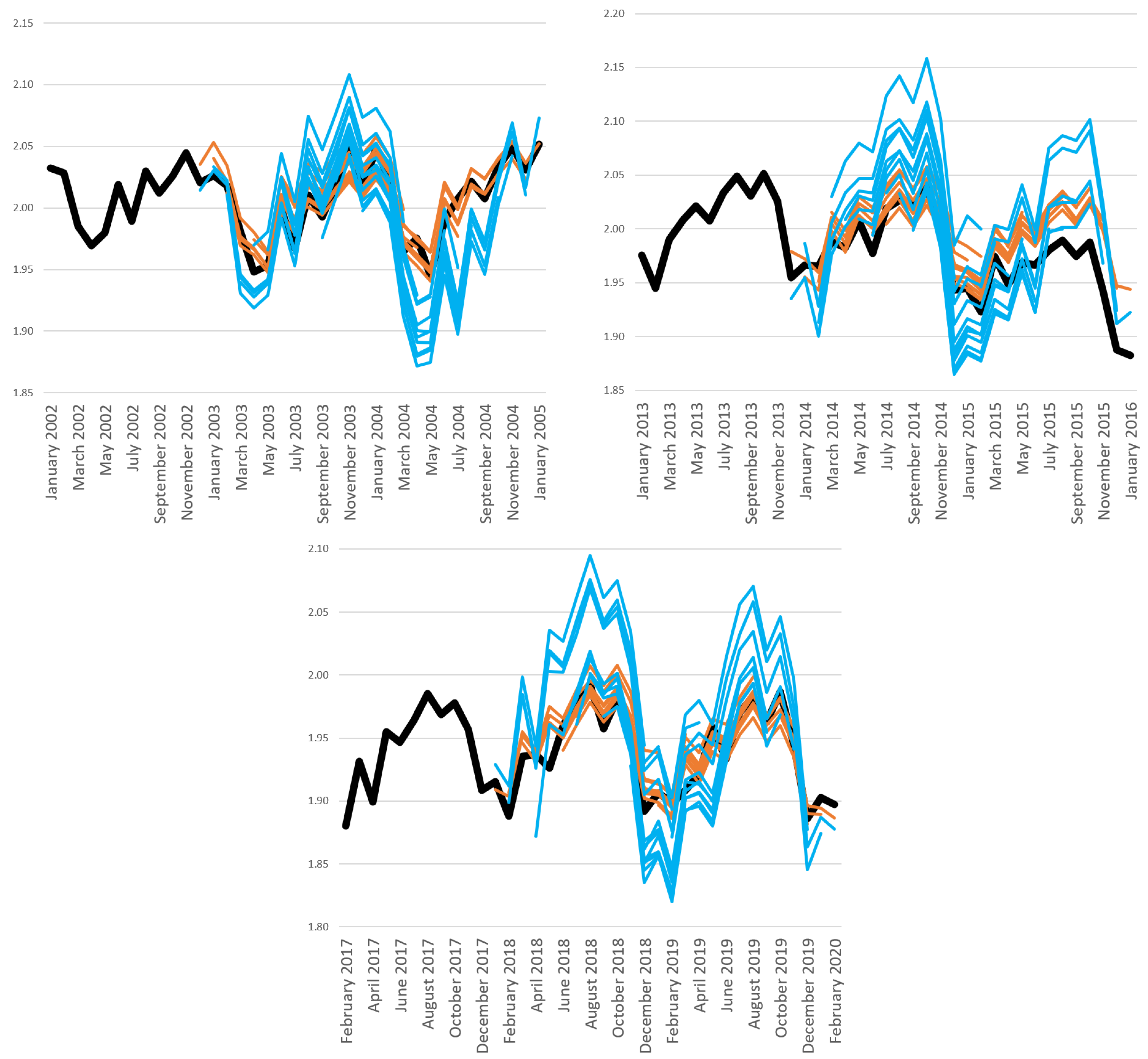
The model that we considered contained 15 lags of the dependent variable. Thus, we used a rolling window of 100 fixed observations for each estimation. We analyzed a recursive forecast horizon that was one to twelve months ahead. We had 91 rolling windows for the general industry forecast series. We re-estimated the model, and we allowed for the best model to be re-specified according to each methodology for each rolling window. We forecasted the production of each sector and used the weight of each sector to obtain the forecasts for the general industry from its components. Our forecast window for analysis ranged from September 2011 to February 2020.

We compared our forecasts with the estimates of four naive models: the AR(1) model, the AR(13) model, the TVP-AR(1) model, and the UC-SV model. All the models were estimated using the data for the general industry (aggregated forecast), the forecast for the general industry from the disaggregated data (disaggregated forecast), or the forecast for the general industry obtained from a combination of an aggregated and a disaggregated series (combination). Thus, we obtained three naive predictions using the AR(1) model (aggregated, disaggregated, and the combination).

We analyzed the forecast performance of the models using the MSE, the MDM test (for details, see Appendix A.6), the MCS from Hansen et al. (2011) (for details, see Appendix A.7), the forecast encompassing test using the implementation in Harvey et al. (1998) (for details, see Appendix A.8), and the multi-horizon forecast comparison via the uSPA and aSPA tests from Quaedvlieg (2021), which are a generalization of Hansen (2005) (for details, see Appendix A.9). We wanted to establish if there was a model that could accurately predict the Brazilian general industrial production index for the period considered. We discuss the results in the next section.

5. Results

This section presents the forecasts of the naive models—AR(1), AR(13), TVP-AR(1), and UC-SV—for one to twelve months ahead as well as the lag selection resulting from the LASSO and its two variants (adaLASSO and WLadaLASSO), ETS, and Autometrics with and without the inclusion of IIS variables. We used these models to forecast the first difference in the logarithm of the general industrial production from aggregated and disaggregated data and from the combination of both. We compared the results according to five aspects: (i) the MSE, (ii) the MDM test, (iii) the MCS, (iv) the forecasting encompassing test, and (v) the aSPA and uSPA tests to determine the model that provides the most accurate forecast.

Table 1. Model Abbreviations.

Abbreviation	Definition
$AR{(1)}^{dis}$	AR(1) with disaggregated series
$AR{(1)}^{ag}$	AR(1) with aggregated series
$AR{(13)}^{dis}$	AR(13) with disaggregated series
$AR{(13)}^{ag}$	AR(13) with aggregated series
$TV{P}^{dis}$	TVP-AR(1) with disaggregated series
$TV{P}^{ag}$	TVP-AR(1) with aggregated series
$UC$-$S{V}^{dis}$	UC-SV with disaggregated series
$UC$-$S{V}^{ag}$	UC-SV with aggregated series
$ET{S}^{dis}$	ETS with disaggregated series
$ET{S}^{ag}$	ETS with aggregated series
$LA{S}^{dis}$	LASSO with disaggregated series
$LA{S}^{ag}$	LASSO with aggregated series
$ad{a}^{dis}$	adaLASSO with disaggregated series
$ad{a}^{ag}$	adaLASSO with aggregated series
$WL{a}^{dis}$	WLadaLASSO with disaggregated series
$WL{a}^{ag}$	WLadaLASSO with aggregated series
$Aut\_n{o}^{dis}$	Autometrics without outlier and with disaggregated series
$Aut\_n{o}^{ag}$	Autometrics without outlier and with aggregated series
$Aut\_II{S}^{dis}$	Autometrics with IIS dummy variables and with disaggregated series
$Aut\_II{S}^{ag}$	Autometrics with IIS dummy variables and with aggregated series
$c\_LAS\_ada$	Combination with LASSO to select and use adaLASSO forecasts
$c\_LAS\_Aut\_no$	Combination with LASSO to select and use $Aut\_no$ forecasts
$c\_LAS\_Aut\_IIS$	Combination with LASSO to select and use $Aut\_IIS$ forecasts
$c\_LAS\_LAS$	Combination with LASSO to select and use LASSO forecasts
$c\_LAS\_TVP$	Combination with LASSO to select and use TVP-AR(1) forecasts
$c\_LAS\_UC$-$SV$	Combination with LASSO to select and use UC-SV forecasts
$c\_LAS\_WLa$	Combination with LASSO to select and use WLadaLASSO forecasts
$c\_LAS\_ETS$	Combination with LASSO to select and use ETS forecasts
$c\_LAS\_AR(1)$	Combination with LASSO to select and use AR(1) forecasts
$c\_ada\_ada$	Combination with adaLASSO to select and use adaLASSO forecasts
$c\_ada\_Aut\_no$	Combination with adaLASSO to select and use $Aut\_no$ forecasts
$c\_ada\_Aut\_IIS$	Combination with adaLASSO to select and use $Aut\_IIS$ forecasts
$c\_ada\_LAS$	Combination with adaLASSO to select and use LASSO forecasts
$c\_ada\_TVP$	Combination with adaLASSO to select and use TVP-AR(1) forecasts
$c\_ada\_UC$-$SV$	Combination with adaLASSO to select and use UC-SV forecasts
$c\_ada\_WLa$	Combination with adaLASSO to select and use WLadaLASSO forecasts
$c\_ada\_ETS$	Combination with adaLASSO to select and use ETS forecasts
$c\_ada\_AR(1)$	Combination with adaLASSO to select and use AR(1) forecasts
$c\_Aut\_ada$	Combination with Autometrics to select and use adaLASSO forecasts
$c\_Aut\_Aut\_no$	Combination with Autometrics to select and use $Aut\_no$ forecasts
$c\_Aut\_Aut\_IIS$	Combination with Autometrics to select and use $Aut\_IIS$ forecasts
$c\_Aut\_LAS$	Combination with Autometrics to select and use LASSO forecasts
$c\_Aut\_TVP$	Combination with Autometrics to select and use TVP-AR(1) forecasts
$c\_Aut\_UC$-$SV$	Combination with Autometrics to select and use UC-SV forecasts
$c\_Aut\_WLa$	Combination with Autometrics to select and use WLadaLASSO forecasts
$c\_Aut\_ETS$	Combination with Autometrics to select and use ETS forecasts
$c\_Aut\_AR(1)$	Combination with Autometrics to select and use AR(1) forecasts

shows the acronyms that we used in this section to describe the models.

Table 2. MSE forecasting results for one to twelve months ahead for different models.

Models	1	2	3	4	5	6	7	8	9	10	11	12
$AR{(1)}^{dis}$	4.01	4.12	4.22	4.28	4.31	4.33	4.34	4.33	4.32	4.33	4.33	4.33
$AR{(1)}^{ag}$	4.24	4.26	4.32	4.35	4.37	4.37	4.37	4.36	4.35	4.35	4.35	4.35
$AR{(13)}^{dis}$	1.21	1.41	1.51	1.59	1.65	1.68	1.70	1.71	1.72	1.72	1.73	1.73
$AR{(13)}^{ag}$	1.39	1.61	1.70	1.78	1.86	1.90	1.91	1.93	1.94	1.95	1.96	1.96
$TV{P}^{dis}$	5.27	5.29	5.70	5.96	6.05	6.12	6.11	6.08	5.94	5.74	5.52	5.30
$TV{P}^{ag}$	5.31	5.31	5.71	5.96	6.03	6.09	6.06	6.01	5.86	5.65	5.44	5.24
$UC$-$S{V}^{dis}$	5.02	7.51	8.34	8.81	9.13	9.35	9.50	9.62	9.70	9.73	9.77	9.80
$UC$-$S{V}^{ag}$	4.97	7.44	8.29	8.77	9.08	9.31	9.47	9.59	9.66	9.70	9.74	9.77
$ET{S}^{dis}$	0.16	0.19	0.21	0.21	0.22	0.22	0.22	0.22	0.22	0.22	0.22	0.22
$ET{S}^{ag}$	0.16	0.19	0.21	0.21	0.22	0.22	0.22	0.22	0.22	0.22	0.23	0.23
$LA{S}^{dis}$	1.25	1.40	1.49	1.58	1.64	1.67	1.69	1.70	1.71	1.72	1.74	1.75
$LA{S}^{ag}$	1.58	1.72	1.81	1.92	2.01	2.05	2.06	2.08	2.09	2.09	2.09	2.09
$ad{a}^{dis}$	1.25	1.40	1.49	1.57	1.63	1.66	1.68	1.70	1.71	1.72	1.74	1.75
$ad{a}^{ag}$	1.62	1.74	1.83	1.94	2.01	2.04	2.05	2.08	2.08	2.08	2.09	2.09
$WL{a}^{dis}$	1.24	1.38	1.47	1.55	1.60	1.63	1.66	1.67	1.69	1.70	1.71	1.72
$WL{a}^{ag}$	1.59	1.75	1.86	1.97	2.05	2.09	2.11	2.13	2.14	2.14	2.14	2.15
$Aut\_n{o}^{dis}$	1.78	1.76	1.76	1.79	1.81	1.81	1.81	1.81	1.82	1.82	1.82	1.83
$Aut\_n{o}^{ag}$	2.04	2.01	1.93	1.97	1.97	1.99	2.00	1.99	1.98	1.96	1.95	1.94
$Aut\_II{S}^{dis}$	2.00	2.06	2.27	2.94	2.72	2.56	2.60	2.51	2.50	2.45	2.45	2.42
$Aut\_II{S}^{ag}$	2.16	2.28	2.50	3.19	3.05	2.95	3.05	2.94	2.93	2.92	2.90	2.90
$c\_LAS\_ada$	1.27	1.42	1.51	1.60	1.66	1.70	1.72	1.74	1.76	1.77	1.79	1.81
$c\_LAS\_Aut\_no$	1.84	1.82	1.83	1.86	1.88	1.89	1.89	1.89	1.89	1.90	1.91	1.92
$c\_LAS\_Aut\_IIS$	1.97	2.03	2.26	2.76	2.58	2.46	2.50	2.42	2.41	2.38	2.37	2.35
$c\_LAS\_LAS$	1.27	1.42	1.52	1.61	1.67	1.71	1.73	1.74	1.76	1.77	1.79	1.80
$c\_LAS\_TVP$	4.89	4.93	5.30	5.56	5.64	5.71	5.70	5.67	5.53	5.35	5.15	4.96
$c\_LAS\_UC$-$SV$	4.74	4.57	4.76	4.92	4.96	5.01	4.98	4.95	4.86	4.72	4.63	4.51
$c\_LAS\_WLa$	1.25	1.40	1.49	1.57	1.63	1.66	1.69	1.71	1.73	1.75	1.77	1.78
$c\_LAS\_ETS$	3.22	2.68	2.52	2.44	2.40	2.36	2.34	2.32	2.31	2.30	2.30	2.29
$c\_LAS\_AR(1)$	3.79	3.92	4.02	4.08	4.12	4.13	4.14	4.14	4.13	4.13	4.14	4.14
$c\_ada\_ada$	1.29	1.44	1.53	1.61	1.67	1.70	1.73	1.75	1.77	1.79	1.81	1.82
$c\_ada\_Aut\_no$	1.92	1.88	1.89	1.91	1.93	1.93	1.92	1.93	1.93	1.94	1.95	1.95
$c\_ada\_Aut\_IIS$	2.05	2.10	2.34	2.86	2.67	2.55	2.59	2.50	2.50	2.46	2.45	2.43
$c\_ada\_LAS$	1.28	1.44	1.53	1.62	1.68	1.72	1.74	1.76	1.77	1.79	1.81	1.82
$c\_ada\_TVP$	4.98	5.03	5.42	5.69	5.78	5.85	5.84	5.81	5.67	5.48	5.28	5.08
$c\_ada\_UC$-$SV$	4.88	4.71	4.91	5.07	5.12	5.17	5.14	5.11	5.00	4.86	4.76	4.63
$c\_ada\_WLa$	1.27	1.41	1.50	1.57	1.63	1.67	1.69	1.72	1.74	1.76	1.78	1.80
$c\_ada\_ETS$	3.18	2.65	2.49	2.42	2.38	2.34	2.32	2.30	2.29	2.28	2.28	2.27
$c\_ada\_AR(1)$	3.86	4.00	4.11	4.17	4.21	4.22	4.23	4.23	4.22	4.22	4.22	4.22
$c\_Aut\_ada$	1.48	1.63	1.71	1.81	1.94	2.04	2.06	2.07	2.12	2.14	2.12	2.12
$c\_Aut\_Aut\_no$	2.03	1.89	1.93	1.97	2.08	2.15	2.14	2.13	2.15	2.16	2.16	2.17
$c\_Aut\_Aut\_IIS$	1.98	1.90	1.97	2.38	2.32	2.28	2.24	2.19	2.23	2.21	2.24	2.20
$c\_Aut\_LAS$	1.54	1.69	1.76	1.85	1.98	2.07	2.08	2.09	2.14	2.15	2.13	2.13
$c\_Aut\_TVP$	4.63	4.29	4.32	4.37	4.42	4.55	4.53	4.57	4.54	4.40	4.29	4.20
$c\_Aut\_UC$-$SV$	4.50	4.02	3.92	3.98	3.98	4.11	4.12	4.16	4.18	4.08	4.05	4.00
$c\_Aut\_WLa$	1.47	1.63	1.70	1.80	1.92	2.02	2.03	2.05	2.10	2.11	2.10	2.10
$c\_Aut\_ETS$	3.81	3.22	3.03	2.93	2.85	2.80	2.78	2.75	2.76	2.74	2.73	2.71
$c\_Aut\_AR(1)$	3.55	3.54	3.53	3.55	3.63	3.70	3.68	3.67	3.65	3.64	3.64	3.61

presents the MSE for the forecast of the first difference in the logarithm of industrial production $\mathsf{\Delta }{y}_{t+h}$, one to twelve months ahead for the different models. We multiplied the MSE value by ${10}^3$ to improve the visualization of the results reported in Table 2. We also reported the lowest MSE value per forecast horizon (bold). The ETS model resulted in a lower MSE compared to the other models forecasting the first difference in the logarithm of industrial production for all of the forecast horizons. This is not an unprecedented result in the literature. Elliott and Timmermann (2008) determined that ETS led to a lower MSE to forecast US inflation and a value-weighted portfolio of US stocks when disregarding combination forecasts.9 In general, one can see that the MSE is smaller for the models with disaggregated series compared to the models with aggregated series; this is independent of the forecast horizon, except for TVP-AR(1), UC-SV, and the Autometrics algorithm when considering IIS dummy variables. The model with the lowest MSE for the forecast for one and two months ahead is the aggregated ETS model, but the difference in the MSE is small compared to the disaggregated ETS. Forecasts with the disaggregated ETS present the lowest MSE for all of the other forecast horizons. The TVP-AR(1) model has the worst forecasting performance based on the MSE, regardless of whether the series is aggregated or disaggregated.

Except for ETS models, the procedure with the smallest MSE is WLadaLASSO with disaggregation for all of the studied forecast horizons—the disaggregated AR(13) model has lower MSE than disaggregated WLadaLASSO only for the forecast (of one month ahead). The combination of the aggregated and disaggregated series with the lowest MSE is the c_LAS_WLa model for all of the forecast horizons; this model relies on LASSO to select the most relevant variables in the combination and uses the disaggregated WLadaLASSO forecasts to make predictions. However, this combination leads to a larger MSE than the disaggregated WLadaLASSO does for all the forecast horizons. Even the combination with the lowest MSE has less accurate predictions than the model with the best forecast, excluding the ETS models. Our result—that the combination of the disaggregated and aggregated series does not lead to the best forecast—is similar to the finding by Faust and Wright (2013). However, our result is the opposite of Hendry and Hubrich (2011) and Weber and Zika (2016).

The difference in the MSE between the LASSO models and their variants is small when using disaggregated data; the disaggregated WLadaLASSO performs better than the other disaggregated LASSO-type methods for the different forecast horizons. However, when we estimated the aggregate models, the LASSO model presented better prediction performance compared to its variants until the forecast horizon five months ahead. The aggregated adaLASSO model resulted in a smaller forecast error by the MSE when the forecast horizon was over five months ahead. It would be interesting to find out why WLadaLASSO does not perform better than its variants with aggregate data or why there is this difference in performance between aggregated and disaggregated data. Konzen and Ziegelmann (2016) pointed out that WLadaLASSO forecasts better than LASSO and adaLASSO when the sample is small, and when there is a large number of lags. In the present study, we have a large number of lags; this does not change between using aggregated or disaggregated WLadaLASSO or other LASSO-type methods.

The difference in the MSE does not allow us to state if the forecast from the disaggregated ETS has higher accuracy statistically compared to other methods. Therefore, we analyzed the results of the MDM test. To perform the test, we established the disaggregated ETS as the benchmark model because it has the lowest MSE when the forecast horizon is three to twelve months ahead. We compared the forecast errors of all of the models with those of the benchmark using the MDM test. The null hypothesis of the test is the equal forecast accuracy between the two models. Under the null hypothesis, the disaggregated ETS forecasts performed as well as the analyzed model. The alternative hypothesis indicates that the forecast of the disaggregated ETS is more accurate statistically.

Table A2. Test for prediction accuracy between models with test statistics and p-values for one to twelve months ahead for different models.

Models	1	2	3	4	5	6	7	8	9	10	11	12
$AR{(1)}^{dis}$	−6.32	−7.32	−9.68	−8.53	−11.28	−12.42	−49.47	−7.32	−7.29	−7.31	−7.26	−7.16
	(0.00)	(0.00)	(0.00)	(0.00)	(0.00)	(0.00)	(0.00)	(0.00)	(0.00)	(0.00)	(0.00)	(0.00)
$AR{(1)}^{ag}$	−6.31	−7.36	−9.69	−8.60	−11.36	−12.43	−48.81	−7.32	−7.29	−7.30	−7.26	−7.15
	(0.00)	(0.00)	(0.00)	(0.00)	(0.00)	(0.00)	(0.00)	(0.00)	(0.00)	(0.00)	(0.00)	(0.00)
$AR{(13)}^{dis}$	−6.51	−5.41	−5.30	−4.72	−4.87	−5.07	−5.68	−6.68	−7.33	−9.77	−11.81	−14.62
	(0.00)	(0.00)	(0.00)	(0.00)	(0.00)	(0.00)	(0.00)	(0.00)	(0.00)	(0.00)	(0.00)	(0.00)
$AR{(13)}^{ag}$	−6.03	−5.31	−4.88	−3.81	−3.94	−4.07	−4.72	−5.55	−6.58	−10.42	−11.00	−13.60
	(0.00)	(0.00)	(0.00)	(0.00)	(0.00)	(0.00)	(0.00)	(0.00)	(0.00)	(0.00)	(0.00)	(0.00)
$TV{P}^{dis}$	−7.28	−7.27	−10.90	−10.47	−7.26	−16.76	−7.41	−8.37	−6.89	−16.22	−11.66	−8.55
	(0.00)	(0.00)	(0.00)	(0.00)	(0.00)	(0.00)	(0.00)	(0.00)	(0.00)	(0.00)	(0.00)	(0.00)
$TV{P}^{ag}$	−6.86	−7.30	−11.08	−10.44	−7.38	−14.97	−7.46	−8.39	−6.97	−15.83	−11.91	−8.47
	(0.00)	(0.00)	(0.00)	(0.00)	(0.00)	(0.00)	(0.00)	(0.00)	(0.00)	(0.00)	(0.00)	(0.00)
$UC$-$S{V}^{dis}$	−8.00	−7.10	−6.56	−7.56	−8.41	−8.93	−8.65	−10.07	−13.25	−14.08	−10.11	−14.24
	(0.00)	(0.00)	(0.00)	(0.00)	(0.00)	(0.00)	(0.00)	(0.00)	(0.00)	(0.00)	(0.00)	(0.00)
$UC$-$S{V}^{ag}$	−7.41	−7.02	−6.51	−7.57	−8.57	−9.17	−8.63	−10.14	−12.72	−14.43	−10.12	−15.82
	(0.00)	(0.00)	(0.00)	(0.00)	(0.00)	(0.00)	(0.00)	(0.00)	(0.00)	(0.00)	(0.00)	(0.00)
$ET{S}^{ag}$	0.11	−0.02	−0.13	−0.72	−1.01	−1.51	−0.87	−1.44	−1.77	−0.95	−4.75	−0.54
	(0.54)	(0.49)	(0.45)	(0.24)	(0.16)	(0.07)	(0.19)	(0.08)	(0.04)	(0.17)	(0.00)	(0.29)
$LA{S}^{dis}$	−6.51	−5.01	−4.85	−4.66	−4.80	−5.01	−5.48	−6.31	−6.79	−7.47	−7.99	−9.27
	(0.00)	(0.00)	(0.00)	(0.00)	(0.00)	(0.00)	(0.00)	(0.00)	(0.00)	(0.00)	(0.00)	(0.00)
$LA{S}^{ag}$	−6.76	−4.85	−4.71	−4.08	−3.97	−4.03	−4.83	−5.14	−5.84	−8.97	−8.53	−8.04
	(0.00)	(0.00)	(0.00)	(0.00)	(0.00)	(0.00)	(0.00)	(0.00)	(0.00)	(0.00)	(0.00)	(0.00)
$ad{a}^{dis}$	−6.44	−5.14	−4.97	−4.65	−4.84	−5.05	−5.66	−6.57	−7.51	−8.48	−9.40	−11.93
	(0.00)	(0.00)	(0.00)	(0.00)	(0.00)	(0.00)	(0.00)	(0.00)	(0.00)	(0.00)	(0.00)	(0.00)
$ad{a}^{ag}$	−6.35	−4.93	−4.84	−4.54	−4.62	−4.81	−5.27	−6.05	−8.88	−14.46	−12.65	−8.70
	(0.00)	(0.00)	(0.00)	(0.00)	(0.00)	(0.00)	(0.00)	(0.00)	(0.00)	(0.00)	(0.00)	(0.00)
$WL{a}^{dis}$	−6.33	−5.08	−5.10	−4.62	−4.67	−5.11	−5.58	−6.44	−7.23	−7.85	−9.13	−12.64
	(0.00)	(0.00)	(0.00)	(0.00)	(0.00)	(0.00)	(0.00)	(0.00)	(0.00)	(0.00)	(0.00)	(0.00)
$WL{a}^{ag}$	−6.46	−5.06	−4.96	−4.54	−4.53	−4.71	−5.11	−5.98	−8.86	−13.08	−11.52	−9.12
	(0.00)	(0.00)	(0.00)	(0.00)	(0.00)	(0.00)	(0.00)	(0.00)	(0.00)	(0.00)	(0.00)	(0.00)
$Aut\_n{o}^{dis}$	−7.21	−6.59	−6.92	−7.05	−7.11	−7.70	−7.61	−8.24	−7.83	−6.76	−6.08	−6.52
	(0.00)	(0.00)	(0.00)	(0.00)	(0.00)	(0.00)	(0.00)	(0.00)	(0.00)	(0.00)	(0.00)	(0.00)
$Aut\_n{o}^{ag}$	−5.82	−6.48	−6.90	−5.76	−5.39	−5.26	−5.71	−4.88	−5.67	−5.13	−4.41	−4.95
	(0.00)	(0.00)	(0.00)	(0.00)	(0.00)	(0.00)	(0.00)	(0.00)	(0.00)	(0.00)	(0.00)	(0.00)
$Aut\_II{S}^{dis}$	−5.50	−5.04	−5.44	−2.51	−4.84	−3.40	−1.78	−2.61	−2.23	−2.32	−2.24	−2.43
	(0.00)	(0.00)	(0.00)	(0.01)	(0.00)	(0.00)	(0.04)	(0.01)	(0.01)	(0.01)	(0.01)	(0.01)
$Aut\_II{S}^{ag}$	−6.03	−4.43	−4.93	−2.49	−4.09	−4.30	−2.11	−3.03	−2.44	−2.94	−2.94	−2.93
	(0.00)	(0.00)	(0.00)	(0.01)	(0.00)	(0.00)	(0.02)	(0.00)	(0.01)	(0.00)	(0.00)	(0.00)
$c\_LAS\_ada$	−6.51	−5.45	−5.28	−4.98	−5.19	−5.26	−5.83	−6.52	−7.20	−7.94	−9.09	−12.92
	(0.00)	(0.00)	(0.00)	(0.00)	(0.00)	(0.00)	(0.00)	(0.00)	(0.00)	(0.00)	(0.00)	(0.00)
$c\_LAS\_Aut\_no$	−7.27	−6.68	−7.11	−7.35	−7.42	−7.62	−7.50	−7.82	−7.26	−6.52	−6.06	−6.16
	(0.00)	(0.00)	(0.00)	(0.00)	(0.00)	(0.00)	(0.00)	(0.00)	(0.00)	(0.00)	(0.00)	(0.00)
$c\_LAS\_Aut\_IIS$	−5.80	−5.51	−5.80	−2.81	−5.09	−3.41	−1.87	−2.92	−2.34	−2.43	−2.42	−2.62
	(0.00)	(0.00)	(0.00)	(0.00)	(0.00)	(0.00)	(0.03)	(0.00)	(0.01)	(0.01)	(0.01)	(0.01)
$c\_LAS\_LAS$	−6.64	−5.35	−5.18	−4.95	−5.11	−5.22	−5.60	−6.26	−6.57	−7.17	−7.81	−10.14
	(0.00)	(0.00)	(0.00)	(0.00)	(0.00)	(0.00)	(0.00)	(0.00)	(0.00)	(0.00)	(0.00)	(0.00)
$c\_LAS\_TVP$	−7.25	−7.49	−10.72	−10.59	−7.37	−15.25	−7.52	−8.37	−6.97	−14.25	−10.91	−46.46
	(0.00)	(0.00)	(0.00)	(0.00)	(0.00)	(0.00)	(0.00)	(0.00)	(0.00)	(0.00)	(0.00)	(0.00)
$c\_LAS\_UC$-$SV$	−8.05	−7.68	−10.41	−8.92	−7.17	−12.03	−7.38	−98.73	−6.88	−36.35	−15.21	−7.59
	(0.00)	(0.00)	(0.00)	(0.00)	(0.00)	(0.00)	(0.00)	(0.00)	(0.00)	(0.00)	(0.00)	(0.00)
$c\_LAS\_WLa$	−6.45	−5.38	−5.38	−4.93	−5.01	−5.32	−5.79	−6.42	−6.94	−7.37	−8.69	−13.89
	(0.00)	(0.00)	(0.00)	(0.00)	(0.00)	(0.00)	(0.00)	(0.00)	(0.00)	(0.00)	(0.00)	(0.00)
$c\_LAS\_ETS$	−8.72	−6.76	−8.05	−8.56	−9.75	−10.65	−11.82	−10.42	−17.75	−27.30	−7.47	−7.35
	(0.00)	(0.00)	(0.00)	(0.00)	(0.00)	(0.00)	(0.00)	(0.00)	(0.00)	(0.00)	(0.00)	(0.00)
$c\_LAS\_AR(1)$	−6.41	−7.42	−9.53	−8.64	−11.23	−12.03	−27.44	−39.87	−7.40	−7.40	−7.33	−7.24
	(0.00)	(0.00)	(0.00)	(0.00)	(0.00)	(0.00)	(0.00)	(0.00)	(0.00)	(0.00)	(0.00)	(0.00)
$c\_ada\_ada$	−6.52	−5.57	−5.38	−5.15	−5.31	−5.33	−5.85	−6.50	−6.89	−7.28	−8.07	−10.05
	(0.00)	(0.00)	(0.00)	(0.00)	(0.00)	(0.00)	(0.00)	(0.00)	(0.00)	(0.00)	(0.00)	(0.00)
$c\_ada\_Aut\_no$	−7.30	−6.79	−7.17	−7.39	−7.36	−7.41	−7.19	−7.36	−6.80	−6.25	−5.73	−5.77
	(0.00)	(0.00)	(0.00)	(0.00)	(0.00)	(0.00)	(0.00)	(0.00)	(0.00)	(0.00)	(0.00)	(0.00)
$c\_ada\_Aut\_IIS$	−5.62	−5.51	−5.84	−2.83	−5.00	−3.29	−1.86	−2.93	−2.27	−2.39	−2.38	−2.58
	(0.00)	(0.00)	(0.00)	(0.00)	(0.00)	(0.00)	(0.03)	(0.00)	(0.01)	(0.01)	(0.01)	(0.01)
$c\_ada\_LAS$	−6.62	−5.47	−5.26	−5.13	−5.25	−5.31	−5.57	−6.21	−6.31	−6.61	−7.07	−8.56
	(0.00)	(0.00)	(0.00)	(0.00)	(0.00)	(0.00)	(0.00)	(0.00)	(0.00)	(0.00)	(0.00)	(0.00)
$c\_ada\_TVP$	−7.19	−7.50	−10.90	−10.53	−7.41	−15.82	−7.50	−8.36	−6.99	−15.29	−11.05	−33.03
	(0.00)	(0.00)	(0.00)	(0.00)	(0.00)	(0.00)	(0.00)	(0.00)	(0.00)	(0.00)	(0.00)	(0.00)
$c\_ada\_UC$-$SV$	−8.02	−7.73	−10.41	−8.87	−7.15	−12.00	−7.36	−8.15	−6.90	−56.69	−15.26	−7.55
	(0.00)	(0.00)	(0.00)	(0.00)	(0.00)	(0.00)	(0.00)	(0.00)	(0.00)	(0.00)	(0.00)	(0.00)
$c\_ada\_WLa$	−6.47	−5.48	−5.47	−5.09	−5.12	−5.37	−5.79	−6.38	−6.65	−6.81	−7.74	−10.51
	(0.00)	(0.00)	(0.00)	(0.00)	(0.00)	(0.00)	(0.00)	(0.00)	(0.00)	(0.00)	(0.00)	(0.00)
$c\_ada\_ETS$	−8.73	−6.77	−8.05	−8.49	−9.81	−10.73	−11.90	−10.48	−18.05	−24.88	−7.45	−7.33
	(0.00)	(0.00)	(0.00)	(0.00)	(0.00)	(0.00)	(0.00)	(0.00)	(0.00)	(0.00)	(0.00)	(0.00)
$c\_ada\_AR(1)$	−6.39	−7.45	−9.65	−8.63	−11.27	−12.35	−36.83	−7.41	−7.38	−7.36	−7.31	−7.24
	(0.00)	(0.00)	(0.00)	(0.00)	(0.00)	(0.00)	(0.00)	(0.00)	(0.00)	(0.00)	(0.00)	(0.00)
$c\_Aut\_ada$	−6.03	−5.12	−5.64	−5.02	−4.61	−4.01	−5.15	−3.78	−4.58	−8.13	−9.89	−6.13
	(0.00)	(0.00)	(0.00)	(0.00)	(0.00)	(0.00)	(0.00)	(0.00)	(0.00)	(0.00)	(0.00)	(0.00)
$c\_Aut\_Aut\_no$	−6.22	−4.68	−5.37	−6.21	−4.71	−4.53	−5.62	−4.41	−6.58	−5.69	−6.00	−5.82
	(0.00)	(0.00)	(0.00)	(0.00)	(0.00)	(0.00)	(0.00)	(0.00)	(0.00)	(0.00)	(0.00)	(0.00)
$c\_Aut\_Aut\_IIS$	−5.28	−4.97	−5.11	−3.57	−3.97	−3.48	−2.54	−2.38	−2.16	−3.32	−2.78	−4.01
	(0.00)	(0.00)	(0.00)	(0.00)	(0.00)	(0.00)	(0.01)	(0.01)	(0.02)	(0.00)	(0.00)	(0.00)
$c\_Aut\_LAS$	−6.32	−4.67	−5.38	−4.96	−4.71	−3.90	−5.53	−4.11	−4.43	−7.57	−6.83	−143.16
	(0.00)	(0.00)	(0.00)	(0.00)	(0.00)	(0.00)	(0.00)	(0.00)	(0.00)	(0.00)	(0.00)	(0.00)
$c\_Aut\_TVP$	−6.81	−5.82	−6.27	−8.09	−8.86	−5.51	−17.62	−17.02	−10.96	−16.10	−7.21	−7.43
	(0.00)	(0.00)	(0.00)	(0.00)	(0.00)	(0.00)	(0.00)	(0.00)	(0.00)	(0.00)	(0.00)	(0.00)
$c\_Aut\_UC$-$SV$	−7.44	−5.95	−5.73	−7.26	−8.31	−4.80	−6.17	−9.62	−5.81	−9.47	−6.99	−5.14
	(0.00)	(0.00)	(0.00)	(0.00)	(0.00)	(0.00)	(0.00)	(0.00)	(0.00)	(0.00)	(0.00)	(0.00)
$c\_Aut\_WLa$	−6.03	−5.18	−5.76	−5.08	−4.60	−3.98	−5.05	−3.78	−4.53	−7.87	−10.42	−29.62
	(0.00)	(0.00)	(0.00)	(0.00)	(0.00)	(0.00)	(0.00)	(0.00)	(0.00)	(0.00)	(0.00)	(0.00)
$c\_Aut\_ETS$	−8.81	−6.38	−7.76	−7.98	−8.62	−8.05	−11.81	−23.83	−6.83	−7.60	−7.16	−7.60
	(0.00)	(0.00)	(0.00)	(0.00)	(0.00)	(0.00)	(0.00)	(0.00)	(0.00)	(0.00)	(0.00)	(0.00)
$c\_Aut\_AR(1)$	−5.99	−5.53	−6.22	−7.49	−6.49	−6.25	−15.61	−10.31	−9.35	−8.58	−13.28	−16.32
	(0.00)	(0.00)	(0.00)	(0.00)	(0.00)	(0.00)	(0.00)	(0.00)	(0.00)	(0.00)	(0.00)	(0.00)

Note: p-values are in parentheses.

in Appendix A.10 presents the MDM statistics and the associated p-values (below the test statistics and in parentheses) for each model compared to the benchmark. We underline and bold the p-value when we do not reject the null hypothesis at 10% statistical significance. From the results of the MDM test, the null hypothesis can be rejected for all models except ETS. The disaggregated ETS shows better forecast performance compared to the naive models (AR(1), AR(13), TVP-AR(1), UC-SV), LASSO and its variants, the Autometrics algorithm, or combinations using aggregated and disaggregated data. However, the disaggregated ETS model is only more accurate than the aggregated ETS for forecast horizons that are six, eight, nine, and eleven months ahead at 10% statistical significance based on the MDM test.

However, the MCS procedure can also be used to determine which models can be considered the best.

Table 3. Model confidence set p-values for one to twelve months ahead for different models.

Models	1	2	3	4	5	6	7	8	9	10	11	12
$AR{(1)}^{dis}$	0.00	0.00	0.00	0.00	0.00	0.00	0.00	0.00	0.00	0.00	0.00	0.00
$AR{(1)}^{ag}$	0.00	0.00	0.00	0.00	0.00	0.00	0.00	0.00	0.00	0.00	0.00	0.00
$AR{(13)}^{dis}$	0.00	0.00	0.00	0.00	0.00	0.00	0.00	0.00	0.00	0.00	0.00	0.00
$AR{(13)}^{ag}$	0.00	0.00	0.00	0.00	0.00	0.00	0.00	0.00	0.00	0.00	0.00	0.00
$TV{P}^{dis}$	0.00	0.00	0.00	0.00	0.00	0.00	0.00	0.00	0.00	0.00	0.00	0.00
$TV{P}^{ag}$	0.00	0.00	0.00	0.00	0.00	0.00	0.00	0.00	0.00	0.00	0.00	0.00
$UC$-$S{V}^{dis}$	0.00	0.00	0.00	0.00	0.00	0.00	0.00	0.00	0.00	0.00	0.00	0.00
$UC$-$S{V}^{ag}$	0.00	0.00	0.00	0.00	0.00	0.00	0.00	0.00	0.00	0.00	0.00	0.00
$ET{S}^{dis}$	0.91	1.00	1.00	1.00	1.00	1.00	1.00	1.00	1.00	1.00	1.00	1.00
$ET{S}^{ag}$	1.00	0.98	0.89	0.62	0.25	0.28	0.37	0.30	0.09	0.28	0.01	0.50
$LA{S}^{dis}$	0.00	0.00	0.00	0.00	0.00	0.00	0.00	0.00	0.00	0.00	0.00	0.00
$LA{S}^{ag}$	0.00	0.00	0.00	0.00	0.00	0.00	0.00	0.00	0.00	0.00	0.00	0.00
$ad{a}^{dis}$	0.00	0.00	0.00	0.00	0.00	0.00	0.00	0.00	0.00	0.00	0.00	0.00
$ad{a}^{ag}$	0.00	0.00	0.00	0.00	0.00	0.00	0.00	0.00	0.00	0.00	0.00	0.00
$WL{a}^{dis}$	0.00	0.00	0.00	0.00	0.00	0.00	0.00	0.00	0.00	0.00	0.00	0.00
$WL{a}^{ag}$	0.00	0.00	0.00	0.00	0.00	0.00	0.00	0.00	0.00	0.00	0.00	0.00
$Aut\_n{o}^{dis}$	0.00	0.00	0.00	0.00	0.00	0.00	0.00	0.00	0.00	0.00	0.00	0.00
$Aut\_n{o}^{ag}$	0.00	0.00	0.00	0.00	0.00	0.00	0.00	0.00	0.00	0.00	0.00	0.00
$Aut\_II{S}^{dis}$	0.00	0.00	0.00	0.00	0.00	0.00	0.01	0.00	0.00	0.00	0.00	0.00
$Aut\_II{S}^{ag}$	0.00	0.00	0.00	0.00	0.00	0.00	0.01	0.00	0.00	0.00	0.00	0.00
$c\_LAS\_ada$	0.00	0.00	0.00	0.00	0.00	0.00	0.00	0.00	0.00	0.00	0.00	0.00
$c\_LAS\_Aut\_no$	0.00	0.00	0.00	0.00	0.00	0.00	0.00	0.00	0.00	0.00	0.00	0.00
$c\_LAS\_Aut\_IIS$	0.00	0.00	0.00	0.00	0.00	0.00	0.02	0.00	0.00	0.00	0.00	0.00
$c\_LAS\_LAS$	0.00	0.00	0.00	0.00	0.00	0.00	0.00	0.00	0.00	0.00	0.00	0.00
$c\_LAS\_TVP$	0.00	0.00	0.00	0.00	0.00	0.00	0.00	0.00	0.00	0.00	0.00	0.00
$c\_LAS\_UC$-$SV$	0.00	0.00	0.00	0.00	0.00	0.00	0.00	0.00	0.00	0.00	0.00	0.00
$c\_LAS\_WLa$	0.00	0.00	0.00	0.00	0.00	0.00	0.00	0.00	0.00	0.00	0.00	0.00
$c\_LAS\_ETS$	0.00	0.00	0.00	0.00	0.00	0.00	0.00	0.00	0.00	0.00	0.00	0.00
$c\_LAS\_AR(1)$	0.00	0.00	0.00	0.00	0.00	0.00	0.00	0.00	0.00	0.00	0.00	0.00
$c\_ada\_ada$	0.00	0.00	0.00	0.00	0.00	0.00	0.00	0.00	0.00	0.00	0.00	0.00
$c\_ada\_Aut\_no$	0.00	0.00	0.00	0.00	0.00	0.00	0.00	0.00	0.00	0.00	0.00	0.00
$c\_ada\_Aut\_IIS$	0.00	0.00	0.00	0.00	0.00	0.00	0.02	0.00	0.00	0.00	0.00	0.00
$c\_ada\_LAS$	0.00	0.00	0.00	0.00	0.00	0.00	0.00	0.00	0.00	0.00	0.00	0.00
$c\_ada\_TVP$	0.00	0.00	0.00	0.00	0.00	0.00	0.00	0.00	0.00	0.00	0.00	0.00
$c\_ada\_UC$-$SV$	0.00	0.00	0.00	0.00	0.00	0.00	0.00	0.00	0.00	0.00	0.00	0.00
$c\_ada\_WLa$	0.00	0.00	0.00	0.00	0.00	0.00	0.00	0.00	0.00	0.00	0.00	0.00
$c\_ada\_ETS$	0.00	0.00	0.00	0.00	0.00	0.00	0.00	0.00	0.00	0.00	0.00	0.00
$c\_ada\_AR(1)$	0.00	0.00	0.00	0.00	0.00	0.00	0.00	0.00	0.00	0.00	0.00	0.00
$c\_Aut\_ada$	0.00	0.00	0.00	0.00	0.00	0.00	0.00	0.00	0.00	0.00	0.00	0.00
$c\_Aut\_Aut\_no$	0.00	0.00	0.00	0.00	0.00	0.00	0.00	0.00	0.00	0.00	0.00	0.00
$c\_Aut\_Aut\_IIS$	0.00	0.00	0.00	0.00	0.00	0.00	0.00	0.00	0.01	0.00	0.00	0.00
$c\_Aut\_LAS$	0.00	0.00	0.00	0.00	0.00	0.00	0.00	0.00	0.00	0.00	0.00	0.00
$c\_Aut\_TVP$	0.00	0.00	0.00	0.00	0.00	0.00	0.00	0.00	0.00	0.00	0.00	0.00
$c\_Aut\_UC$-$SV$	0.00	0.00	0.00	0.00	0.00	0.00	0.00	0.00	0.00	0.00	0.00	0.00
$c\_Aut\_WLa$	0.00	0.00	0.00	0.00	0.00	0.00	0.00	0.00	0.00	0.00	0.00	0.00
$c\_Aut\_ETS$	0.00	0.00	0.00	0.00	0.00	0.00	0.00	0.00	0.00	0.00	0.00	0.00
$c\_Aut\_AR(1)$	0.00	0.00	0.00	0.00	0.00	0.00	0.00	0.00	0.00	0.00	0.00	0.00

presents the MCS p-values for each model. The p-values of the models are in bold if we determine that the model could be included in the set of “best” models with 90% probability. Only ETS models (with aggregated and disaggregated data) were selected. Only the disaggregated ETS model remains in the MCS for forecast horizons that are nine and eleven months ahead.

Next, we used the forecast encompassing test to study whether the disaggregated ETS model forecasts add information compared to forecasts from the other models. We applied the same approach as in Harvey et al. (1998).

Table 4. Forecast encompassing test for one to twelve months ahead for different models using the disaggregated ETS as the benchmark.

	${\widehat{\mathit{\lambda }}}_{\mathbf{dis}}^{\mathit{h}}$
Models	1		2		3		4		5		6		7		8		9		10		11		12
$AR{(1)}^{dis}$	1.0	***	1.0	***	1.0	***	1.0	***	1.0	***	1.0	***	1.0	***	1.1	***	1.1	***	1.1	***	1.1	***	1.1	***
$AR{(1)}^{ag}$	1.0	***	1.0	***	1.0	***	1.0	***	1.0	***	1.0	***	1.0	***	1.1	***	1.1	***	1.1	***	1.1	***	1.1	***
$AR{(13)}^{dis}$	1.2	***	1.2	***	1.2	***	1.2	***	1.2	***	1.2	***	1.2	***	1.2	***	1.2	***	1.2	***	1.2	***	1.2	***
$AR{(13)}^{ag}$	1.2	***	1.2	***	1.2	***	1.2	***	1.2	***	1.2	***	1.2	***	1.2	***	1.2	***	1.2	***	1.2	***	1.2	***
$TV{P}^{dis}$	1.0	***	1.0	***	1.0	***	1.0	***	1.0	***	1.0	***	1.0	***	1.0	***	1.0	***	1.0	***	1.1	***	1.1	***
$TV{P}^{ag}$	1.0	***	1.0	***	1.0	***	1.0	***	1.0	***	1.0	***	1.0	***	1.0	***	1.0	***	1.0	***	1.1	***	1.1	***
$UC$-$S{V}^{dis}$	1.0	***	1.0	***	1.0	***	1.0	***	1.0	***	1.0	***	1.0	***	1.0	***	1.0	***	1.0	***	1.0	***	1.0	***
$UC$-$S{V}^{ag}$	1.0	***	1.0	***	1.0	***	1.0	***	1.0	***	1.0	***	1.0	***	1.0	***	1.0	***	1.0	***	1.0	***	1.0	***
$ET{S}^{ag}$	0.5	*	0.5		0.6		0.8	*	1.2	**	1.2	**	1.0	*	1.1	**	1.5	***	1.0	**	2.0	***	0.9	*
$LA{S}^{dis}$	1.2	***	1.3	***	1.2	***	1.2	***	1.2	***	1.2	***	1.2	***	1.2	***	1.3	***	1.3	***	1.3	***	1.3	***
$LA{S}^{ag}$	1.2	***	1.2	***	1.2	***	1.2	***	1.2	***	1.2	***	1.2	***	1.2	***	1.2	***	1.3	***	1.3	***	1.3	***
$ad{a}^{dis}$	1.2	***	1.2	***	1.2	***	1.2	***	1.2	***	1.2	***	1.2	***	1.2	***	1.3	***	1.3	***	1.3	***	1.3	***
$ad{a}^{ag}$	1.2	***	1.2	***	1.2	***	1.2	***	1.2	***	1.2	***	1.2	***	1.2	***	1.3	***	1.2	***	1.2	***	1.3	***
$WL{a}^{dis}$	1.2	***	1.3	***	1.2	***	1.2	***	1.2	***	1.2	***	1.2	***	1.2	***	1.3	***	1.3	***	1.3	***	1.3	***
$WL{a}^{ag}$	1.2	***	1.2	***	1.2	***	1.2	***	1.2	***	1.2	***	1.2	***	1.2	***	1.2	***	1.2	***	1.2	***	1.2	***
$Aut\_n{o}^{dis}$	1.2	***	1.2	***	1.2	***	1.2	***	1.2	***	1.2	***	1.2	***	1.2	***	1.2	***	1.2	***	1.2	***	1.2	***
$Aut\_n{o}^{ag}$	1.2	***	1.2	***	1.2	***	1.2	***	1.2	***	1.2	***	1.2	***	1.2	***	1.2	***	1.2	***	1.3	***	1.2	***
$Aut\_II{S}^{dis}$	1.1	***	1.1	***	1.1	***	1.0	***	1.2	***	1.2	***	1.1	**	1.2	***	1.2	***	1.2	***	1.2	***	1.2	***
$Aut\_II{S}^{ag}$	1.1	***	1.1	***	1.1	***	1.0	***	1.2	***	1.2	***	1.1	***	1.2	***	1.1	***	1.2	***	1.2	***	1.2	***
$c\_LAS\_ada$	1.2	***	1.2	***	1.2	***	1.2	***	1.2	***	1.2	***	1.2	***	1.2	***	1.2	***	1.2	***	1.2	***	1.2	***
$c\_LAS\_Aut\_no$	1.1	***	1.2	***	1.2	***	1.2	***	1.2	***	1.2	***	1.2	***	1.2	***	1.2	***	1.2	***	1.2	***	1.2	***
$c\_LAS\_Aut\_IIS$	1.1	***	1.1	***	1.1	***	1.0	***	1.2	***	1.2	***	1.1	**	1.2	***	1.2	***	1.2	***	1.2	***	1.2	***
$c\_LAS\_LAS$	1.2	***	1.2	***	1.2	***	1.2	***	1.2	***	1.2	***	1.2	***	1.2	***	1.2	***	1.2	***	1.2	***	1.2	***
$c\_LAS\_TVP$	1.0	***	1.0	***	1.0	***	1.0	***	1.0	***	1.0	***	1.0	***	1.0	***	1.0	***	1.0	***	1.1	***	1.1	***
$c\_LAS\_UC$-$SV$	1.0	***	1.0	***	1.0	***	1.0	***	1.0	***	1.0	***	1.1	***	1.0	***	1.1	***	1.1	***	1.1	***	1.1	***
$c\_LAS\_WLa$	1.2	***	1.2	***	1.2	***	1.2	***	1.2	***	1.2	***	1.2	***	1.2	***	1.2	***	1.2	***	1.2	***	1.2	***
$c\_LAS\_ETS$	1.1	***	1.1	***	1.1	***	1.1	***	1.2	***	1.1	***	1.1	***	1.2	***	1.2	***	1.2	***	1.2	***	1.2	***
$c\_LAS\_AR(1)$	1.1	***	1.0	***	1.0	***	1.0	***	1.1	***	1.0	***	1.1	***	1.1	***	1.1	***	1.1	***	1.1	***	1.1	***
$c\_ada\_ada$	1.2	***	1.2	***	1.2	***	1.2	***	1.2	***	1.2	***	1.2	***	1.2	***	1.2	***	1.2	***	1.2	***	1.2	***
$c\_ada\_Aut\_no$	1.1	***	1.2	***	1.2	***	1.2	***	1.2	***	1.2	***	1.2	***	1.2	***	1.2	***	1.2	***	1.2	***	1.2	***
$c\_ada\_Aut\_IIS$	1.1	***	1.1	***	1.1	***	1.0	***	1.2	***	1.2	***	1.1	**	1.2	***	1.2	***	1.2	***	1.2	***	1.2	***
$c\_ada\_LAS$	1.2	***	1.2	***	1.2	***	1.2	***	1.2	***	1.2	***	1.2	***	1.2	***	1.2	***	1.2	***	1.2	***	1.2	***
$c\_ada\_TVP$	1.0	***	1.0	***	1.0	***	1.0	***	1.0	***	1.0	***	1.0	***	1.0	***	1.0	***	1.0	***	1.1	***	1.1	***
$c\_ada\_UC$-$SV$	1.0	***	1.0	***	1.0	***	1.0	***	1.0	***	1.0	***	1.1	***	1.0	***	1.1	***	1.1	***	1.1	***	1.1	***
$c\_ada\_WLa$	1.2	***	1.2	***	1.2	***	1.2	***	1.2	***	1.2	***	1.2	***	1.2	***	1.2	***	1.2	***	1.2	***	1.2	***
$c\_ada\_ETS$	1.1	***	1.1	***	1.1	***	1.1	***	1.2	***	1.1	***	1.1	***	1.2	***	1.2	***	1.2	***	1.2	***	1.2	***
$c\_ada\_AR(1)$	1.0	***	1.0	***	1.0	***	1.0	***	1.1	***	1.0	***	1.0	***	1.1	***	1.1	***	1.1	***	1.1	***	1.1	***
$c\_Aut\_ada$	1.2	***	1.2	***	1.2	***	1.2	***	1.2	***	1.2	***	1.2	***	1.2	***	1.2	***	1.2	***	1.3	***	1.2	***
$c\_Aut\_Aut\_no$	1.1	***	1.2	***	1.2	***	1.2	***	1.2	***	1.2	***	1.2	***	1.2	***	1.2	***	1.2	***	1.2	***	1.2	***
$c\_Aut\_Aut\_IIS$	1.1	***	1.1	***	1.2	***	1.1	***	1.3	***	1.2	***	1.2	***	1.2	***	1.2	**	1.3	***	1.2	***	1.3	***
$c\_Aut\_LAS$	1.2	***	1.2	***	1.2	***	1.2	***	1.2	***	1.2	***	1.2	***	1.2	***	1.2	***	1.2	***	1.3	***	1.2	***
$c\_Aut\_TVP$	1.1	***	1.0	***	1.0	***	1.1	***	1.1	***	1.1	***	1.1	***	1.0	***	1.1	***	1.1	***	1.1	***	1.1	***
$c\_Aut\_UC$-$SV$	1.1	***	1.0	***	1.0	***	1.1	***	1.1	***	1.1	***	1.1	***	1.0	***	1.1	***	1.1	***	1.0	***	1.1	***
$c\_Aut\_WLa$	1.2	***	1.2	***	1.2	***	1.2	***	1.2	***	1.2	***	1.2	***	1.2	***	1.2	***	1.3	***	1.3	***	1.2	***
$c\_Aut\_ETS$	1.1	***	1.1	***	1.1	***	1.1	***	1.1	***	1.1	***	1.1	***	1.1	***	1.1	***	1.1	***	1.1	***	1.1	***
$c\_Aut\_AR(1)$	1.1	***	1.1	***	1.1	***	1.1	***	1.1	***	1.1	***	1.1	***	1.1	***	1.1	***	1.1	***	1.1	***	1.1	***

Note: *, **, *** denote statistical significance at the 10%, 5%, and 1% levels, respectively.

reports the estimated weights ${\widehat{\lambda }}_{dis}^h$ and the associated statistical significance of the encompassing analysis considering the disaggregated ETS as the benchmark (presented in bold if we did not reject the null hypothesis that the disaggregated ETS model forecast does not contain information that is useful for forecasting the first difference in industrial production beyond the information already found in the other model at 10% statistical significance). Excluding the aggregated ETS, all of the estimated weights for the disaggregated ETS model are equal to or above one and are statistically significant at 1% for all forecast horizons. All of the models, regardless of whether they used aggregated or disaggregated data or a combination, do not provide significant additional information relative to the forecast of the disaggregated ETS model, except for the aggregated ETS model. In other words, the optimal combination forecast only incorporates information from the disaggregated ETS model at any horizon, except for the aggregated ETS model. The forecasts based on the disaggregated ETS model always encompass the forecasts based on models other than ETS.

Considering the aggregated ETS model as the exception, we analyzed the weights associated with the disaggregated and the aggregated ETS. We estimated a convex combination of the two forecasts as

$$y_{t+h}^h={\lambda }_{dis}^h{\widehat{y}}_{dis,t+h}^h+{\lambda }_{ag}^h{\widehat{y}}_{ag,t+h}^h$$

(11)

Table A3. Forecast encompassing tests between aggregated and disaggregated ETS with ${\widehat{\lambda }}_{dis}^h$ (${\widehat{\lambda }}_{ag}^h$) and the disaggregated (aggregated) ETS weights.

Horizon	${\widehat{\mathit{\lambda }}}_{\mathbf{ag}}^{\mathit{h}}$	${\widehat{\mathit{\lambda }}}_{\mathbf{dis}}^{\mathit{h}}$
1	0.53 **	0.47 *
2	0.48	0.52
3	0.41	0.59
4	0.22	0.78 *
5	−0.25	1.25 **
6	−0.17	1.17 **
7	0.02	0.98 *
8	−0.08	1.08 **
9	−0.51	1.51 ***
10	−0.01	1.01 **
11	−0.97	1.97 ***
12	0.09	0.91 *

Note: *, **, *** denote statistical significance at 10%, 5%, and 1% levels, respectively.

in Appendix A.10 reports the estimated weights of ${\widehat{\lambda }}_{dis}^h$ and ${\widehat{\lambda }}_{ag}^h$ and the associated statistical significance of the encompassing analysis that only considers the ETS model. The weight of ${\widehat{\lambda }}_{dis}^h$ is statistically significant at 10% for all horizons, except for those two and three months ahead. The majority of 1 ${\widehat{\lambda }}_{dis}^h$ is equal to one for forecast horizons greater than four, and the optimal combination forecast provided by (11) only incorporates information from the disaggregated ETS model for these forecast horizons. This points to the disaggregated ETS model having superior informational content compared to the aggregated version of the model. The weight ${\widehat{\lambda }}_{ag}^h$ is only statistically significant at 5% for one period ahead. For forecast horizons greater than one, the weight for the aggregated ETS model is statistically zero.

Finally, we analyzed the forecasts of each model for all of the horizons together using the uSPA and aSPA tests and compared them to the forecast of the ETS model with disaggregated data, which was used as the benchmark. This is different from what we discussed earlier, in which we looked at each time horizon separately. The results of the uSPA and aSPA tests are reported in

Table 5. aSPA and uSPA tests for a multi-horizon forecast comparison with all 12 horizons together.

	uSPA		aSPA
Models	t Statistics	p-Value	t Statistics	p-Value
$AR{(1)}^{dis}$	7.724	0.000	29.404	0.000
$AR{(1)}^{ag}$	7.758	0.000	29.522	0.000
$AR{(13)}^{dis}$	4.810	0.000	11.127	0.000
$AR{(13)}^{ag}$	4.768	0.000	9.783	0.001
$TV{P}^{dis}$	7.539	0.000	28.050	0.000
$TV{P}^{ag}$	7.431	0.000	28.734	0.000
$UC$-$S{V}^{dis}$	7.189	0.000	16.878	0.000
$UC$-$S{V}^{ag}$	7.127	0.000	17.065	0.000
$ET{S}^{ag}$	−0.124	0.003	2.722	0.009
$LA{S}^{dis}$	4.731	0.000	11.025	0.000
$LA{S}^{ag}$	4.159	0.000	9.134	0.001
$ad{a}^{dis}$	4.830	0.000	11.240	0.001
$ad{a}^{ag}$	4.778	0.000	10.155	0.000
$WL{a}^{dis}$	4.773	0.000	11.284	0.000
$WL{a}^{ag}$	4.761	0.000	9.746	0.001
$Aut\_n{o}^{dis}$	6.549	0.000	14.215	0.000
$Aut\_n{o}^{ag}$	5.637	0.000	10.512	0.001
$Aut\_II{S}^{dis}$	2.455	0.000	4.659	0.002
$Aut\_II{S}^{ag}$	2.940	0.000	5.151	0.002
$c\_LAS\_ada$	5.077	0.000	11.562	0.000
$c\_LAS\_Aut\_no$	6.715	0.000	14.349	0.000
$c\_LAS\_Aut\_IIS$	2.576	0.000	5.090	0.001
$c\_LAS\_LAS$	4.962	0.000	11.308	0.001
$c\_LAS\_TVP$	7.518	0.000	28.717	0.000
$c\_LAS\_UC$-$SV$	7.502	0.000	28.987	0.000
$c\_LAS\_WLa$	4.993	0.000	11.635	0.000
$c\_LAS\_ETS$	6.934	0.000	20.147	0.000
$c\_LAS\_AR(1)$	7.856	0.000	27.967	0.000
$c\_ada\_ada$	5.229	0.000	11.606	0.000
$c\_ada\_Aut\_no$	6.705	0.000	13.912	0.000
$c\_ada\_Aut\_IIS$	2.556	0.000	5.033	0.001
$c\_ada\_LAS$	5.229	0.000	11.606	0.000
$c\_ada\_TVP$	7.510	0.000	29.496	0.000
$c\_ada\_UC$-$SV$	7.549	0.000	29.223	0.000
$c\_ada\_WLa$	5.127	0.000	11.658	0.000
$c\_ada\_ETS$	6.917	0.000	20.114	0.000
$c\_ada\_AR(1)$	7.846	0.000	29.007	0.000
$c\_Aut\_ada$	3.805	0.000	10.468	0.000
$c\_Aut\_Aut\_no$	4.854	0.000	11.488	0.000
$c\_Aut\_Aut\_IIS$	3.103	0.000	6.388	0.001
$c\_Aut\_LAS$	3.805	0.000	10.468	0.000
$c\_Aut\_TVP$	5.941	0.000	15.168	0.000
$c\_Aut\_UC$-$SV$	4.469	0.000	11.117	0.000
$c\_Aut\_WLa$	3.754	0.000	10.347	0.000
$c\_Aut\_ETS$	6.832	0.000	19.809	0.000
$c\_Aut\_AR(1)$	5.903	0.000	16.763	0.000

. When considering all 12 horizons together, we rejected the null hypothesis of equal predictability for all models for both tests at 1% statistical significance. Together, the multi-horizon results are different from the single-horizon results. Previously, we (i) determined that the ETS model with aggregated data had a lower MSE in the first two-time horizons; (ii) only rejected the null hypothesis of equal predictability between the ETS models with aggregated and disaggregated data using the MDM test for 4 of the 12 horizons; and (iii) determined that the MCS contained the ETS model with aggregated data for 10 of the 12 horizons. However, we determined that the ETS model with disaggregated data was the best compared to all of the other models, according to the uSPA and aSPA tests when considering all 12 horizons together at 1% statistical significance.

By considering the multi-horizon together, we can determine the horizon at which the ETS model with disaggregated data becomes the best model to forecast when comparing only with the aggregated ETS—because it is the model with the most accurate forecasts by the MSE in addition to the disaggregated ETS itself. For this, we conducted the aSPA and uSPA tests recursively by considering the horizons together. For example, we first analyzed the tests for $h=1$ only, and then reported the tests with $h=1$ and $h=2$ together, and so on. We report the results of the uSPA and aSPA tests comparing the ETS models using aggregated and disaggregated data while considering the horizons together in

Table 6. Comparison between ETS models with aggregated and disaggregated data with a multi-horizon analysis.

	uSPA		aSPA
Horizons	t-Statistics	p-Value	t-Statistics	p-Value
1	−0.124	0.612	−0.124	0.617
1,2	−0.124	0.407	−0.073	0.574
1,2,3	−0.124	0.280	0.014	0.488
1,2,3,4	−0.124	0.196	0.171	0.361
1,…,5	−0.124	0.153	0.506	0.165
1,…,6	−0.124	0.088	0.783	0.101
1,…,7	−0.124	0.065	0.912	0.081
1,…,8	−0.124	0.028	1.189	0.049
1,…,9	−0.124	0.016	1.715	0.025
1,…,10	−0.124	0.010	2.003	0.019
1,…,11	−0.124	0.005	2.727	0.009
1,…,12	−0.124	0.003	2.722	0.009

, in which rejection at 10% statistical significance is in bold. At 10% statistical significance, we can say that the ETS model with disaggregated data becomes the best model after six forecast horizons (jointly with the uSPA test) or after seven forecast horizons (jointly with the aSPA test). It is important to remember that we rejected the null hypothesis of equal predictability between the ETS models using aggregated and disaggregated data after six horizons in the MDM test results in Table A2 at 10% statistical significance. Based on the aSPA test, we can say that the forecast provided by the ETS model disaggregated over the longer forecast horizons—for example, six and seven horizons—compensates for worse performances over the shorter forecast horizons—for example, one and two horizons—considering a total of seven horizons.

Comparing the Forecast of the Disaggregated ETS Model with That of the Disaggregated WLadaLASSO

In this subsection, we want to determine why the ETS model performs better in forecasting industrial production in Brazil.10 In Figure 2, we compare the forecasts for one to twelve months made by the disaggregated ETS model (orange line) and the disaggregated WLadaLASSO (light blue line) model, which was determined to be the best model according to MSE apart from the ETS model. Fifteen orange lines represent the disaggregated ETS forecast for one to twelve months because each line represents forecasts, i.e., one step, two steps, etc., up to twelve steps ahead for the disaggregated ETS model for one rolling window. For example, the upper left figure considers the period from January 2002 to January 2005 and reports the forecasts of 15 rolling windows for the disaggregated ETS. In addition, the thick black line presents the realization of the logarithm for general industrial production in Brazil. We divided it into three periods to improve the visualization of results.

In Figure 2, we can see that the forecast of the ETS model follows the trend and seasonality of the logarithm of industrial production more closely. In addition, the WLadaLASSO forecasts tend to indicate a stronger increase (decrease) in the series than in the observed series over the three periods. The comparison of the model forecasts with the observed series does not lead to many changes in the three periods, showing the superiority of the forecast provided by the ETS model. The ETS model is an adaptive scheme, and the other methods are not. Additionally, we can see a change in the series pattern in the upper right figure with the forecast period being 2012 because there was a break in 2014, the beginning of the recession in Brazil, and there was another recession in 2016, the impeachment of President Dilma Rousseff, where there was a break in the trend (no-trend).

6. Conclusions

The present work sought to analyze two points regarding how to forecast industrial production in Brazil. First, we compared different univariate models to select the lags using LASSO and two of its variants, ETS models, and the Autometrics algorithm. Among these models, we studied which model was best able to forecast industrial production in Brazil. Second, we considered whether aggregated or disaggregated data or the combination of the two led to better forecasting accuracy for general industrial production.

Our results indicated that the ETS model was able to provide a better forecast. This model was also the best for forecasting US inflation and the US stock portfolio in Elliott and Timmermann (2008) if we disregarded the combination of forecasts. The ETS with disaggregated data had the smallest MSE across all of the forecast horizons, with the exception of one and two months ahead. We used the ETS model with disaggregated data as the benchmark for the MDM test. We rejected the null hypothesis of forecast accuracy equality for all of the models except for the aggregated ETS model based on the MDM test result. The disaggregated ETS model only demonstrated the same forecasting performance as the aggregated ETS for forecast horizons of one to five, seven, ten, and twelve months ahead. Our results indicate the importance of modeling the series separately when forecasting industrial production in Brazil.

In addition, the ETS with the disaggregated series was included in the set of “best” models with 90% probability for all forecast horizons based on the MCS. This was also the case for the ETS model using the aggregate series for all the forecast horizons, except for those nine and eleven months ahead. These were the only two models included in the MCS. The MCS also included the ETS model using the aggregate series even when the modified Diebold and Mariano (1995) test indicated that it performed worse compared to the disaggregated ETS, such as in the case with forecast horizons that were six and eight months ahead.

The combination of the aggregated and disaggregated series did not lead to a better forecast than when only the disaggregated series was considered by the ETS model. This is in contrast to Hendry and Hubrich (2011) and Weber and Zika (2016), but similar to Faust and Wright (2013).

Epprecht et al. (2021) obtained different results than we did and determined that adaLASSO and the Autometrics algorithm demonstrated similar forecasting performance with a small number of relevant variables and when the candidate variables were lower than the number of observations. In our case, the LASSO models and variants performed better than the Autometrics algorithm in general, even when the number of candidate variables was lower than the number of observations. In addition, we used a recursive forecast, in which the Autometrics algorithm presented better results compared to those obtained by Kock and Teräsvirta (2014).

We investigated the forecasts of each model for all of the horizons together by using the uSPA and aSPA tests differently than we did before. We rejected the null hypothesis of equal predictability between the disaggregated ETS model and all of the other models for both tests at 1% statistical significance while considering all 12 horizons together. These multi-horizon results were different from what we were able to obtain with just one horizon. We can say that the ETS model with disaggregated data is the best model to forecast horizons from six or seven periods onward, together, depending on the test compared to the aggregated ETS. This is because we do not reject the null hypothesis of equal predictability between aggregated and disaggregated ETS models at 10% statistical significance in case we consider up to the sixth forecast horizon together (or the seventh, depending on the test version).

We also analyzed forecast encompassing tests to investigate whether the other models reported relevant information in their forecasts for the optimal combination forecasts compared to the disaggregated ETS model. Except for the aggregated ETS model, the optimal combination forecast only incorporated information from the disaggregated ETS model compared to models other than ETS. In such cases, the optimal combination forecast was simply the forecast of the disaggregated ETS model, except when we considered the aggregated ETS model, because the disaggregated ETS model forecast contains all the information that is useful for forecasting the first difference in industrial production compared to the other models. The aggregated ETS forecasts add relevant information that is statistically significant at 5% for only one period ahead compared to the disaggregated ETS model. For one period ahead only, the optimal combination forecast includes the aggregated ETS forecasts with positive weight. The disaggregated ETS introduced information for forecasting industrial production for six horizons among the 12 that were analyzed compared to the aggregated ETS model at 5% statistical significance. Additionally, the estimated weight for the disaggregated ETS model was close to or greater than one in nine of the twelve horizons analyzed compared to the aggregated ETS model. That is, the optimal combination forecast included only the forecast of the disaggregated ETS model in these forecast horizons. We can say that disaggregated ETS model forecasts are informationally superior.

As an extension of the present work, we will compare these results with the robust forecasting11 devices described by Castle et al. (2015) and the smoothed robust forecasting techniques found in Martinez et al. (2022). According to these studies, the use of the ETS would not be the best option. Additionally, we will consider the Card procedure proposed by Doornik et al. (2020), which performed better than ETS in Makridakis et al. (2020), to determine if this improves the forecast accuracies of our models. However, this comparison will only be possible when the new version of OxMetrics^™ (Doornik and Hendry (2022)) is released.

References

1. Aguiar, Mark, and Gita Gopinath. 2007. Emerging market business cycles: The cycle is the trend. Journal of Political Economy 115: 69–102. [Google Scholar] [CrossRef] [Green Version]
2. Albert, Jim. 2009. Bayesian Computation with R. Berlin: Springer. [Google Scholar]
3. Andrews, Donald W. K. 1991. Heteroskedasticity and autocorrelation consistent covariance matrix estimation. Econometrica: Journal of the Econometric Society 59: 817–58. [Google Scholar] [CrossRef]
4. Barhoumi, Karim, Olivier Darné, and Laurent Ferrara. 2010. Are disaggregate data useful for factor analysis in forecasting French GDP? Journal of Forecasting 29: 132–44. [Google Scholar] [CrossRef] [Green Version]
5. Barnett, Alina, Haroon Mumtaz, and Konstantinos Theodoridis. 2014. Forecasting UK GDP growth and inflation under structural change. a comparison of models with time-varying parameters. International Journal of Forecasting 30: 129–43. [Google Scholar] [CrossRef]
6. Bhattacharya, Utpal, and Neal Galpin. 2011. The global rise of the value-weighted portfolio. Journal of Financial and Quantitative Analysis 46: 737–56. [Google Scholar] [CrossRef]
7. Blake, Andrew P., and Haroon Mumtaz. 2017. Applied Bayesian Econometrics for Central Bankers. Technical Report. London: Bank of England. [Google Scholar]
8. Borup, Daniel, and Erik Christian Montes Schütte. 2022. In search of a job: Forecasting employment growth using Google Trends. Journal of Business & Economic Statistics 40: 186–200. [Google Scholar]
9. Bulligan, Guido, Roberto Golinelli, and Giuseppe Parigi. 2010. Forecasting monthly industrial production in real-time: From single equations to factor-based models. Empirical Economics 39: 303–36. [Google Scholar] [CrossRef]
10. Carlo, Thiago Carlomagno, and Emerson Fernandes Marçal. 2016. Forecasting Brazilian inflation by its aggregate and disaggregated data: A test of predictive power by forecast horizon. Applied Economics 48: 4846–60. [Google Scholar] [CrossRef]
11. Carstensen, Kai, Klaus Wohlrabe, and Christina Ziegler. 2011. Predictive ability of business cycle indicators under test: A case study for the Euro area industrial production. Journal of Economics and Statistics (Jahrbuecher fuer Nationaloekonomie und Statistik) 231: 82–106. [Google Scholar]
12. Carter, Chris K., and Robert Kohn. 1994. On Gibbs sampling for state space models. Biometrika 81: 541–53. [Google Scholar] [CrossRef]
13. Castle, Jennifer L., Jurgen A. Doornik, and David F. Hendry. 2011. Evaluating Automatic Model Selection. Journal of Time Series Econometrics 3: 1–33. [Google Scholar] [CrossRef] [Green Version]
14. Castle, Jennifer L., Michael P. Clements, and David F. Hendry. 2015. Robust approaches to forecasting. International Journal of Forecasting 31: 99–112. [Google Scholar] [CrossRef] [Green Version]
15. Chib, Siddhartha. 1995. Marginal likelihood from the Gibbs output. Journal of the American Statistical Association 90: 1313–21. [Google Scholar] [CrossRef]
16. Chong, Yock Y., and David F. Hendry. 1986. Econometric evaluation of linear macro-economic models. The Review of Economic Studies 53: 671–90. [Google Scholar] [CrossRef]
17. Clements, Michael P., and David F. Hendry. 1993. On the limitations of comparing mean square forecast errors. Journal of Forecasting 12: 617–37. [Google Scholar] [CrossRef]
18. Diebold, Francis, and Roberto Mariano. 1995. Comparing predictive accuracy. Journal of Business & Economic Statistics 13: 253–63. [Google Scholar]
19. Doornik, Jurgen A. 2008. Encompassing and Automatic Model Selection. Oxford Bulletin of Economics and Statistics 70: 915–25. [Google Scholar] [CrossRef]
20. Doornik, Jurgen A., and David F. Hendry. 2022. Empirical Econometric Modellig—PcGive 16: Volume 1. London: Timberlake Consultants. [Google Scholar]
21. Doornik, Jurgen A., Jennifer L. Castle, and David F. Hendry. 2020. Card forecasts for M4. International Journal of Forecasting 36: 129–34. [Google Scholar] [CrossRef]
22. Elliott, Graham, and Allan Timmermann. 2008. Economic forecasting. Journal of Economic Literature 46: 3–56. [Google Scholar] [CrossRef]
23. Epprecht, Camila, Dominique Guegan, Álvaro Veiga, and Joel Correa da Rosa. 2021. Variable selection and forecasting via automated methods for linear models: Lasso/adalasso and autometrics. Communications in Statistics-Simulation and Computation 50: 103–22. [Google Scholar] [CrossRef] [Green Version]
24. Ericsson, Neil R. 1992. Parameter constancy, mean square forecast errors, and measuring forecast performance: An exposition, extensions, and illustration. Journal of Policy Modeling 14: 465–95. [Google Scholar] [CrossRef] [Green Version]
25. Espasa, Antoni, Eva Senra, and Rebeca Albacete. 2002. Forecasting inflation in the european monetary union: A disaggregated approach by countries and by sectors. The European Journal of Finance 8: 402–21. [Google Scholar] [CrossRef] [Green Version]
26. Faust, Jon, and Jonathan H. Wright. 2013. Forecasting inflation. In Handbook of Economic Forecasting. Amsterdam: Elsevier, vol. 2, pp. 2–56. [Google Scholar]
27. Ghysels, Eric, and Massimiliano Marcellino. 2018. Applied Economic Forecasting Using Time Series Methods. Oxford: Oxford University Press. [Google Scholar]
28. Giacomini, Raffaella. 2015. Economic theory and forecasting: Lessons from the literature. The Econometrics Journal 18: C22–C41. [Google Scholar] [CrossRef] [Green Version]
29. Giacomini, Raffaella, and Barbara Rossi. 2010. Forecast comparisons in unstable environments. Journal of Applied Econometrics 25: 595–620. [Google Scholar] [CrossRef]
30. Giacomini, Raffaella, and Clive W. J. Granger. 2004. Aggregation of space-time processes. Journal of Econometrics 118: 7–26. [Google Scholar] [CrossRef] [Green Version]
31. Granger, Clive W. J. 1987. Implications of aggregation with common factors. Econometric Theory 3: 208–22. [Google Scholar] [CrossRef]
32. Hansen, Peter R. 2005. A test for superior predictive ability. Journal of Business & Economic Statistics 23: 365–80. [Google Scholar] [CrossRef] [Green Version]
33. Hansen, Peter R., Asger Lunde, and James M. Nason. 2011. The model confidence set. Econometrica 79: 453–97. [Google Scholar] [CrossRef] [Green Version]
34. Harvey, David, Stephen Leybourne, and Paul Newbold. 1997. Testing the equality of prediction mean squared errors. International Journal of Forecasting 13: 281–91. [Google Scholar] [CrossRef]
35. Harvey, David I., Stephen J. Leybourne, and Paul Newbold. 1998. Tests for forecast encompassing. Journal of Business & Economic Statistics 16: 254–59. [Google Scholar]
36. Heinisch, Katja, and Rolf Scheufele. 2018. Bottom-up or direct? forecasting German GDP in a data-rich environment. Empirical Economics 54: 705–45. [Google Scholar] [CrossRef] [Green Version]
37. Hendry, David F., and Bent Nielsen. 2007. Econometric Modeling: A Likelihood Approach. Princeton: Princeton University Press. [Google Scholar]
38. Hendry, David F., and Kirstin Hubrich. 2011. Combining disaggregate forecasts or combining disaggregate information to forecast an aggregate. Journal of Business & Economic Statistics 29: 216–27. [Google Scholar]
39. Hubrich, Kirstin. 2005. Forecasting Euro area inflation: Does aggregating forecasts by hicp component improve forecast accuracy? International Journal of Forecasting 21: 119–36. [Google Scholar] [CrossRef] [Green Version]
40. Hyndman, Rob, Anne B. Koehler, J. Keith Ord, and Ralph D. Snyder. 2008. Forecasting with Exponential Smoothing: The State Space Approach. New York: Springer Science & Business Media. [Google Scholar]
41. Hyndman, Robin John, and Yeasmin Khandakar. 2008. Automatic time series forecasting: The forecast package for R. Journal of Statistical Software 27: 1–22. [Google Scholar] [CrossRef] [Green Version]
42. Hyndman, Rob J., Anne B. Koehler, J. Keith Ord, and Ralph D. Snyder. 2005. Prediction intervals for exponential smoothing using two new classes of state space models. Journal of Forecasting 24: 17–37. [Google Scholar] [CrossRef]
43. Hyndman, Rob J., Anne B. Koehler, Ralph D. Snyder, and Simone Grose. 2002. A state space framework for automatic forecasting using exponential smoothing methods. International Journal of forecasting 18: 439–54. [Google Scholar] [CrossRef] [Green Version]
44. Jacquier, Eric, Nicholas G. Polson, and Peter E. Rossi. 2002. Bayesian analysis of stochastic volatility models. Journal of Business & Economic Statistics 20: 69–87. [Google Scholar]
45. Kapetanios, George, Massimiliano Marcellino, and Fabrizio Venditti. 2019. Large time-varying parameter vars: A nonparametric approach. Journal of Applied Econometrics 34: 1027–49. [Google Scholar] [CrossRef]
46. Kock, Anders Bredahl, and Timo Teräsvirta. 2014. Forecasting performances of three automated modelling techniques during the economic crisis 2007–2009. International Journal of Forecasting 30: 616–31. [Google Scholar] [CrossRef]
47. Kohn, David, Fernando Leibovici, and Håkon Tretvoll. 2021. Trade in commodities and business cycle volatility. American Economic Journal: Macroeconomics 13: 173–208. [Google Scholar] [CrossRef]
48. Konzen, Evandro, and Flavio A. Ziegelmann. 2016. Lasso-type penalties for covariate selection and forecasting in time series. Journal of Forecasting 35: 592–612. [Google Scholar] [CrossRef]
49. Kotchoni, Rachidi, Maxime Leroux, and Dalibor Stevanovic. 2019. Macroeconomic forecast accuracy in a data-rich environment. Journal of Applied Econometrics 34: 1050–72. [Google Scholar] [CrossRef]
50. Kroese, Dirk P., and Joshua C. C. Chan. 2014. Statistical Modeling and Computation. Berlin: Springer. [Google Scholar]
51. Lütkepohl, Helmut. 1984. Linear transformations of vector arma processes. Journal of Econometrics 26: 283–93. [Google Scholar] [CrossRef]
52. Lütkepohl, Helmut. 1987. Forecasting Aggregated Vector ARMA Processes. New York: Springer Science & Business Media, vol. 284. [Google Scholar]
53. Makridakis, Spyros, Evangelos Spiliotis, and Vassilios Assimakopoulos. 2020. The M4 competition: 100,000 time series and 61 forecasting methods. International Journal of Forecasting 36: 54–74. [Google Scholar] [CrossRef]
54. Marcellino, Massimiliano, James H. Stock, and Mark W. Watson. 2003. Macroeconomic forecasting in the Euro area: Country specific versus area-wide information. European Economic Review 47: 1–18. [Google Scholar] [CrossRef]
55. Martinez, Andrew B., Jennifer L. Castle, and David F. Hendry. 2022. Smooth robust multi-horizon forecasts. In Essays in Honor of M. Hashem Pesaran: Prediction and Macro Modeling. Bingley: Emerald Publishing Limited, pp. 143–65. [Google Scholar]
56. Ord, John Keith, Anne B. Koehler, and Ralph D. Snyder. 1997. Estimation and prediction for a class of dynamic nonlinear statistical models. Journal of the American Statistical Association 92: 1621–29. [Google Scholar] [CrossRef]
57. Park, Heewon, and Fumitake Sakaori. 2013. Lag weighted lasso for time series model. Computational Statistics 28: 493–504. [Google Scholar] [CrossRef]
58. Pesaran, M. Hashem, Richard G. Pierse, and Mohan S. Kumar. 1989. Econometric analysis of aggregation in the context of linear prediction models. Econometrica: Journal of the Econometric Society 57: 861–88. [Google Scholar] [CrossRef]
59. Picchetti, Paulo. 2018. Brazilian business cycles as characterized by CODACE. In Business Cycles in BRICS. Cham: Springer International Publishing, pp. 331–35. [Google Scholar] [CrossRef]
60. Pretis, Felix, J. James Reade, and Genaro Sucarrat. 2018. Automated general-to-specific (GETS) regression modeling and indicator saturation for outliers and structural breaks. Journal of Statistical Software 86: 1–44. [Google Scholar] [CrossRef]
61. Quaedvlieg, Rogier. 2021. Multi-horizon forecast comparison. Journal of Business & Economic Statistics 39: 40–53. [Google Scholar]
62. Rapach, David E., Matthew C. Ringgenberg, and Guofu Zhou. 2016. Short interest and aggregate stock returns. Journal of Financial Economics 121: 46–65. [Google Scholar] [CrossRef]
63. Rossi, Barbara, and Tatevik Sekhposyan. 2010. Have economic models’ forecasting performance for us output growth and inflation changed over time, and when? International Journal of Forecasting 26: 808–35. [Google Scholar] [CrossRef]
64. Stock, James H., and Mark W. Watson. 2002. Macroeconomic forecasting using diffusion indexes. Journal of Business & Economic Statistics 20: 147–62. [Google Scholar]
65. Stock, James H., and Mark W. Watson. 2007. Why has US inflation become harder to forecast? Journal of Money, Credit and Banking 39: 3–33. [Google Scholar] [CrossRef] [Green Version]
66. Talagala, Thiyanga S., Rob J. Hyndman, and George Athanasopoulos. 2018. Meta-learning how to forecast time series. Monash Econometrics and Business Statistics Working Papers 6: 16. [Google Scholar]
67. Tibshirani, Robert. 1996. Regression shrinkage and selection via the LASSO. Journal of the Royal Statistical Society: Series B (Methodological) 58: 267–88. [Google Scholar] [CrossRef]
68. Van Garderen, Kees Jan, Kevin Lee, and M. Hashem Pesaran. 2000. Cross-sectional aggregation of non-linear models. Journal of Econometrics 95: 285–331. [Google Scholar] [CrossRef]
69. Weber, Enzo, and Gerd Zika. 2016. Labour market forecasting in Germany: Is disaggregation useful? Applied Economics 48: 2183–98. [Google Scholar] [CrossRef]
70. Zellner, Arnold, and Justin Tobias. 2000. A note on aggregation, disaggregation and forecasting performance. Journal of Forecasting 19: 457–65. [Google Scholar] [CrossRef]
71. Zou, Hui. 2006. The adaptive Lasso and its Oracle properties. Journal of the American Statistical Association 101: 1418–29. [Google Scholar] [CrossRef] [Green Version]
Figure 1. Time series of the logarithm of general industrial production in Brazil.
Econometrics 10 00027 g001
Figure 2. Comparison of the forecast provided by the disaggregated WLadaLASSO while considering three periods. The thick line is the realization, the light blue line is the disaggregated WLadaLASSO forecast, and the orange line is the disaggregated ETS forecast. The upper left and upper right figures cover the period between January 2002 and January 2005 and between January 2013 and January 2016, respectively, and the lower figure covers the period between February 2017 and February 2020.
Econometrics 10 00027 g002