Some Notes on Maximum Entropy Utility

Abstract

The maximum entropy principle is effective in solving decision problems, especially when it is not possible to obtain sufficient information to induce a decision. Among others, the concept of maximum entropy is successfully used to obtain the maximum entropy utility which assigns cardinal utilities to ordered prospects (consequences). In some cases, however, the maximum entropy principle fails to produce a satisfactory result representing a set of partial preferences properly. Such a case occurs when incorporating ordered utility increments or uncertain probability to the well-known maximum entropy formulation. To overcome such a shortcoming, we propose a distance-based solution, so-called the centralized utility increments which are obtained by minimizing the expected quadratic distance to the set of vertices that varies upon partial preferences. Therefore, the proposed method seeks to determine utility increments that are adjusted to the center of the vertices. Other partial preferences about the prospects and their corresponding centralized utility increments are derived and compared to the maximum entropy utility.

1. Introduction

The maximum entropy principle is effective in solving decision problems, especially when it is not possible to obtain sufficient information to induce a decision [1,2,3,4,5]. Applications of the entropy principle to the multiple criteria decision-making (MCDM) problems can be found in [6,7,8]. Abbas [9] presents a method to assign cardinal utilities to ordered prospects (consequences) in the presence of uncertainty. The ordered prospects which are included in the category of partial preferences are easily encountered in practice [9,10,11]. The use of partial preferences about the prospects can provide a decision-maker with comfort in specifying preferences but in view of decision-making may fail to result in a final decision. Thus, an elegant approach to circumvent this problem is needed to solve real-world decision-making problems. To this end, Abbas [9] developed the maximum entropy approach to assigning cardinal utility to each prospect when only the ordered prospects are known. However, we doubt if the maximum entropy approach results in cardinal utilities representing a set of partial preferences properly where some other partial preferences about the prospects are additionally incorporated. In another context of true maximum ignorance where the state of prior knowledge is not strong, the maximum a posteriori probability can be better estimated by classical Bayesian theory; it is not necessary to introduce a new and exotic approach such as maximum entropy [12].

We discuss the maximum entropy utility approach further using the notations and definitions from Abbas [9].

2. Does the Maximum Entropy Principle Always Guarantee a Good Solution?

A utility vector contains the utility values of prospects starting from the lowest to the highest, where a utility value of zero (one) is assigned to the lowest (highest) according to a von Neumann and Morgenstern type utility assessment. We assume that there is at least one prospect, which has a strict preference to exclude the case of absolute indifference. The utility vector for $\left(K+1\right)$ prospects can be denoted by

$$\begin{array}{cc}\hfill U& \triangleq \left(U_0, U_1,\cdots ,U_{K-1}, U_K\right)\hfill \\ & =\left(0, U_1, U_2,\cdots ,U_{K-1}, 1\right)\hfill \end{array}$$

where $0\le U_1\le U_2\le \cdots \le U_{K-1}\le 1$.

A utility increment vector $\Delta U$, whose elements are equal to the difference between the consecutive elements in the utility vector, can be denoted by

$$\Delta U\triangleq \left(U_1-0, U_2-U_1,\cdots ,1-U_{K-1}\right)=\left(\Delta u_1, \Delta u_2,\Delta u_3,\cdots ,\Delta u_K\right).$$

A utility increment vector $\Delta U$ satisfies two properties: (1) $\Delta u_i\ge 0$, $i=1,\cdots ,K$ and (2) ${{\displaystyle \sum }}_{i=1}^K\Delta u_i=1$. Thus, it represents a point in a $K$-dimensional simplex, so-called the utility simplex. To assign cardinal utility to each $\Delta u_i$, Abbas [9] presumed that “If all we know about the prospects is their ordering, it is reasonable to assume, therefore, that the location of the utility increment vector is uniformly distributed over the utility simplex.” This idea led to the following nonlinear program (Equation (1)) of which the objective function is the maximum entropy constrained by a normalization condition and non-negativity constraints:

$$\begin{array}{ll}\Delta U_{maxent}=& \underset{\Delta u_1, \Delta u_2,\cdots , \Delta u_K }{\mathrm{maximize}}-{{\displaystyle \sum }}_{i=1}^K\Delta u_i\log \left(\Delta u_i\right)\\ \text{such that}& \\ & {{\displaystyle \sum }}_{i=1}^K\Delta u_i=1\\ & \Delta u_i\ge 0,i=1,\cdots ,K.\end{array}$$

(1)

The optimal solution to this program is a utility increment vector with equal increments, that is

$$\Delta u_i=\frac{1}{K},i=1,\cdots ,K.$$

(2)

This result seems to properly represent the utility simplex, since its extreme points simply consist of $K$ unit vectors $e_i$ (one in the ith element and zeroes elsewhere) of which the coordinate-wise average yields $\frac{1}{K}$.

Let us assume an ordered increasing utility (OIU) increment (in the latter part of the paper, we provide the ordered decreasing utility (ODU) increment defined by $\Delta u_1\ge \Delta u_2\ge \cdots \ge \Delta u_K$):

$$\Delta u_1\le \Delta u_2\le \cdots \le \Delta u_K,$$

(3)

which can be further rewritten as $U_1-0\le U_2-U_1 \le \cdots \le 1-U_{K-1}$ in terms of the utility vector. Studies regarding this partial preference, also called comparable preference differences, degree of preference, strength of preference, or preference intensity to utility theory, are found in Fishburn [13] and Sarin [14].

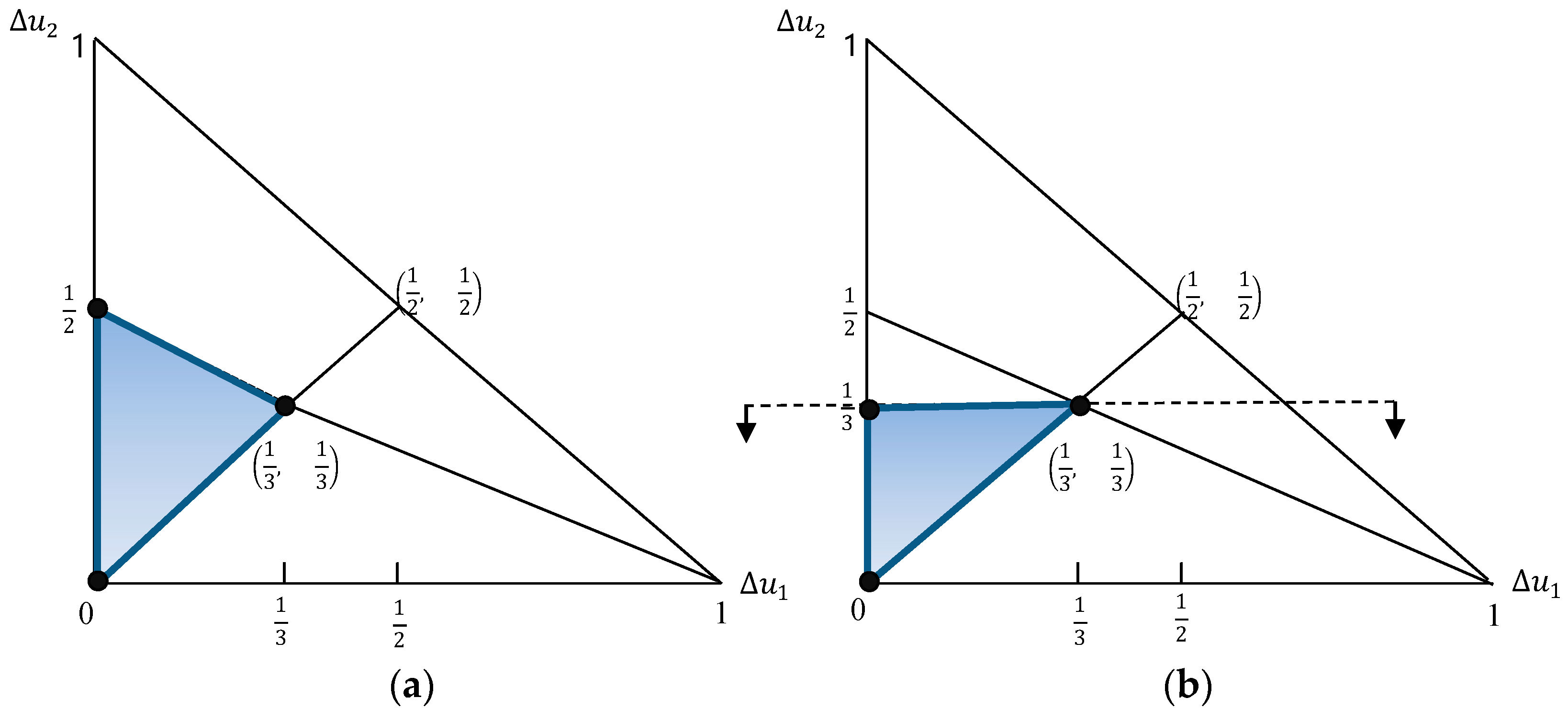
The incorporation of the ordered utility increment vector in the system of constraints of Equation (1) leads to the mathematical program (Equation (4)) and surely restricts the utility simplex as depicted in Figure 1, when considering a case of $K=3$.

$$\begin{array}{ll}\Delta U_{maxent}=& \underset{\Delta u_1, \Delta u_2,\cdots , \Delta u_K }{\mathrm{maximize}}-{{\displaystyle \sum }}_{i=1}^K\Delta u_i\log \left(\Delta u_i\right)\\ \text{such that}& \\ & \Delta u_1\le \Delta u_2\le \cdots \le \Delta u_K\\ & {{\displaystyle \sum }}_{i=1}^K\Delta u_i=1\\ & \Delta u_i\ge 0,i=1,\cdots ,K.\end{array}$$

(4)

The solution to Equation (4) however still yields a utility increment vector with equal increments, $\Delta u_i=\frac{1}{K}$, $i=1,\cdots ,K$ since nothing other than $v_K$ can result in a larger maximum entropy in a set of extreme points $\left\{v_1,v_2,\cdots ,v_K\right\}$ where $v_1=\left(0,0,\cdots 0,0,1\right)$, $v_2=\left(0,0,\cdots ,0,\frac{1}{2},\frac{1}{2}\right)$, $\cdots$, $v_K=\left(\frac{1}{K},\frac{1}{K},\cdots \frac{1}{K},\frac{1}{K}\right)$.

Technically, we always obtain this result when the constituent constraints in the maximum entropy program contain $v_K$ as one of their extreme points. To illustrate, let us incorporate a constraint $\Delta u_3-\Delta u_2\ge \Delta u_2-\Delta u_1$ which more restricts the utility simplex in Figure 1 (see Figure 2). The set of extreme points is composed of $v_1=\left(0,0,1\right)$, $v_2=\left(0,\frac{1}{3},\frac{2}{3}\right)$, $v_3=\left(\frac{1}{3},\frac{1}{3},\frac{1}{3}\right)$, which also leads to a maximum entropy merely anchored at $v_3$.

Therefore, it is doubtable if such equal utility increments adequately represent the feasible region (i.e., the restricted utility simplex) and if the assignment of such values will eventually be valid.

Let us consider another case where the maximum entropy principle does not work properly. We present the discrete version of preference inclusion in the maximum entropy utility, originally dealt with by Abbas [9] in a continuous case. Let us assume that a decision-maker specifies indifference between a lottery $\langle x_1, p_1;x_2, p_2;\cdots ;x_K, p_K\rangle$ and a reference lottery $\langle x_K, p, x_1\rangle$, thus yielding

$${{\displaystyle \sum }}_{i=1}^K{p}_i{U}_i\left(x_i\right)=p\mathrm{where}{x}_1\le x_2\le \cdots \le x_K.$$

(5)

Equation (5) can be rewritten in terms of the utility increments $\Delta u_i$ such that ${{\displaystyle \sum }}_{i=1}^K{F}_{i-1}\Delta u_i=1-p$ where $F_i={{\displaystyle \sum }}_{j=1}^i{p}_j$ ($F_0=0$, $F_K=1)$.

Then, the principle of maximum entropy utility leads to the following program:

$$\begin{array}{ll}\Delta U_{maxent}=& \underset{\Delta u_1, \Delta u_2,\cdots , \Delta u_K }{\mathrm{maximize}}-{{\displaystyle \sum }}_{i=1}^K\Delta u_i\log \left(\Delta u_i\right)\\ \text{such that}& \\ & {{\displaystyle \sum }}_{i=1}^K{F}_{i-1}\Delta u_i=1-p\\ & {{\displaystyle \sum }}_{i=1}^K\Delta u_i=1\\ & \Delta u_i\ge 0,i=1,\cdots ,K.\end{array}$$

(6)

The solution to Equation (6) is obtained by

$$\Delta u_i=\frac{\exp \left(\beta F_{i-1}\right)}{{{\displaystyle \sum }}_{i=1}^K\exp (\beta F_{i-1})}$$

(7)

where $\beta$ corresponds to the Lagrange multiplier and is determined iteratively from the equation ${{\displaystyle \sum }}_{i=1}^K\left(F_{i-1}-\left(1-p\right)\right)\exp (\beta F_{i-1})=0$. A formulation similar to Equation (6) and its solution (Equation (7)) are found in different contexts [15,16,17]. If a decision-maker is uncertain about the probability that equates a discrete lottery with a reference lottery and thus specifies a probability interval $\underset{\_}{p}\le \tilde{p}\le \overline{p}$ as in [18], the expected utility of the prospects in Equation (5) can be expressed in the form of an interval:

$$\underset{\_}{p}\le {{\displaystyle \sum }}_{i=1}^K{p}_i{U}_i\left(x_i\right)\le \overline{p},\mathrm{or}1-\overline{p}\le {{\displaystyle \sum }}_{i=1}^K{F}_{i-1}\Delta u_i\le 1-\underset{\_}{p}.$$

(8)

With Equation (8) added in Equation (1), we obtain the optimal utility increments vector to Equation (9) that is anchored at either the lower or the upper bound in Equation (8).

$$\begin{array}{ll}\Delta U_{maxent}=& \underset{\Delta u_1, \Delta u_2,\cdots , \Delta u_K }{\max }-{{\displaystyle \sum }}_{i=1}^K\Delta u_i\log \left(\Delta u_i\right)\\ \text{such that}& \\ & 1-\overline{p}\le {{\displaystyle \sum }}_{i=1}^K{F}_{i-1}\Delta u_i\le 1-\underset{\_}{p}\\ & {{\displaystyle \sum }}_{i=1}^K\Delta u_i=1\\ & \Delta u_i\ge 0,i=1,\cdots ,K.\end{array}$$

(9)

For example, let $K=5$, $F_i=\frac{i}{5}$, $i=1,\cdots ,5$, and $\tilde{p}\in \left[0.6, 0.7\right]$. Then, if we simply let $\Delta u_i=\frac{1}{5}$ for all $i$, we obtain the maximum entropy value while they satisfy all the constraints in Equation (9), that is, ${{\displaystyle \sum }}_{i=1}^5\frac{F_{i-1}}{5}=0.4=1-\underset{\_}{p}$ and ${{\displaystyle \sum }}_{i=1}^5\frac{1}{5}=1$. Rather than this optimal solution, however, it is more reasonable to expect to obtain utility increments corresponding to somewhere between $\Delta u_i\left(0.6\right)$ and $\Delta u_i\left(0.7\right)$ in Equation (7). Further, this undesirable result is observed while uncertain $\tilde{p}$ varies upon $\left[0.6, 0.6+\alpha \right]$ or $\left[0.6-\alpha , 0.6\right]$, $\alpha >0$.

3. Centralized Utility Increments

We have shown two examples in which the maximum entropy principle works improperly when the utility simplex is restricted by additional partial preferences. This undesirable outcome can be attributed to the fact that the maximum entropy value is always attained when the equal utility increments vector is one of the extreme points characterizing the restricted utility simplex. Clearly, the utility increments representative of the restricted utility simplex are more likely to be found by considering as many extreme points as possible. Toward this end, we propose new utility increments that minimize the sum of the squared distances from all the extreme points (MSDE) to physically locate the utility increments at the center of the restricted utility simplex. Specifically, the MSDE approach considers the utility increments that minimize the expected quadratic distance to the set of vertices that varies upon types of partial preferences. This leads to the MSDE program in Equation (10):

$$\begin{array}{ll}\mathrm{minimize}& {{\displaystyle \sum }}_{i=1}^K{{\displaystyle \sum }}_{j=1}^M{\left(\Delta u_i-v_{ij}\right)}^2\\ \text{such that}& \\ & {{\displaystyle \sum }}_{i=1}^K\Delta u_i=1\\ & \Delta u_i\ge 0,i=1,\cdots ,K\end{array}$$

(10)

where $v_{ij}$ is the $i$th entry of the $j$th extreme point for the ordered prospects and $M$ is the number of extreme points.

The solution to Equation (10) yields

$$\Delta u_i=\frac{1}{M}{{\displaystyle \sum }}_{j=1}^M{v}_{ij}=\frac{1}{K}$$

(11)

since $M=K$ and $v_j=e_j$ for all $j$.

This result is identical to Equation (2), which is compatible with the maximum entropy utility under the utility simplex. If we add the ordered utility increment vector (Equation (3)) to the system of constraints in Equation (10), the MSDE yields a solution:

$$\Delta u_i=\frac{1}{K}{{\displaystyle \sum }}_{j=K-i+1}^K\frac{1}{j},i=1,\cdots ,K$$

(12)

since $v_1=\left(0,\cdots ,0,1\right)$, $v_2=\left(0,\cdots ,0,\frac{1}{2},\frac{1}{2}\right)$, $\cdots$, $v_K=\left(\frac{1}{K},\cdots ,\frac{1}{K},\frac{1}{K}\right)$.

This solution, so-called the centralized utility increments, is quite different from the equal increments that would have resulted had we solved the program using the maximum entropy principle. In the case of $K=3$, simply compare $\left(\frac{2}{18}, \frac{5}{18}, \frac{11}{18}\right)$ based on the centralized utility increments with $\left(\frac{1}{3}, \frac{1}{3}, \frac{1}{3}\right)$ based on the maximum entropy principle.

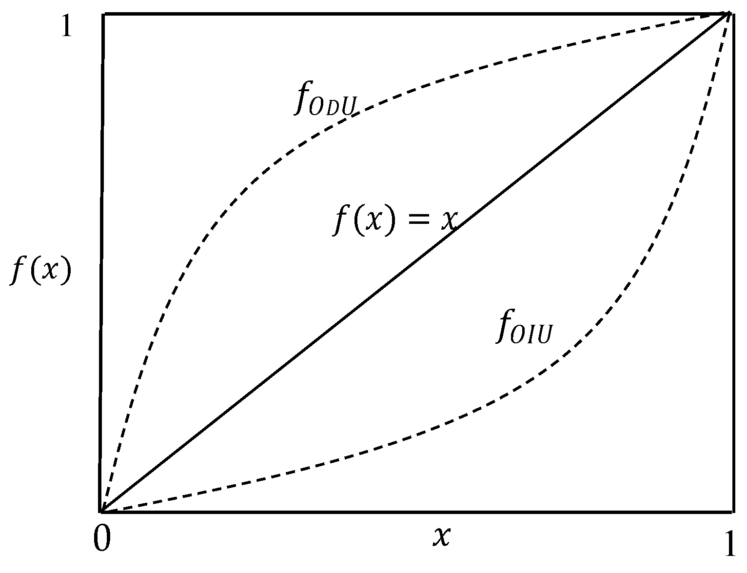
To show that the solution in Equation (12) truly represents the center of vertices of the restricted utility simplex, we first develop a cumulative discrete utility increments function for $\Delta u_i$, $F\left(\frac{i}{K}\right)={{\displaystyle \sum }}_{j=1}^i\Delta u_j$, $i=1,\cdots ,K$ and then its continuous function as follows [19]:

$$f_{OIU}\left(x\right)=\{\begin{array}{c}x+\left(1-x\right)\ln \left(1-x\right) \mathrm{for} 0\le x<1\\ 0 \mathrm{for} x=1\end{array}.$$

(13)

Similar computations yield a continuous function for ordered decreasing utility increments as follows:

$$f_{ODU}\left(x\right)=\{\begin{array}{c}x\left(1-\ln x\right) \mathrm{for} 0<x\le 1\\ 0 \mathrm{for} x=0\end{array}.$$

(14)

It is interesting to note that both $f_{OIU}\left(x\right)$ and $f_{ODU}\left(x\right)$ include the entropy expression $-x\ln x$ as their component. As shown in Figure 3, the continuous functions $f_{OIU}\left(x\right)$ and $f_{ODU}\left(x\right)$ bisect the lower triangle and upper triangle (of an area of $\frac{1}{2}$) respectively since ${{\displaystyle \int }}_0^1{f}_{OIU}\left(x\right)dx=\frac{1}{4}$ and ${{\displaystyle \int }}_0^1{f}_{ODU}\left(x\right)dx=\frac{3}{4}$. Noting that the straight line $f\left(x\right)=x$ generates equal increments (for $\Delta u_i=\frac{1}{K}$, $F\left(\frac{i}{K}\right)={{\displaystyle \sum }}_{j=1}^i\Delta u_j=\frac{i}{K}$ and $\underset{K\to \infty }{lim}{F}_K\left(x\right)=f\left(x\right)=$) for any $K$, $f_{OIU}\left(x\right)$ produces the centralized utility increments among numerous continuous functions that generate the utility increments satisfying $\Delta u_1\le \Delta u_2\le \cdots \le \Delta u_K$.

Further, we consider two categories of partial utility values that are widely used in MCDM problems: loose articulation (i.e., open-ended partial preferences of utility values) and interval expressions of utility values. The open-ended partial preferences of utility values may include the following types of preferences (see Ahn [20]):

• Weak preference of utility values (WPU): $U_{WPU}=\left\{U_i\ge U_{i-1},i=1,\cdots ,K\right\}$
• Strict preference of utility values (SPU): $U_{SPU}=\{U_i-U_{i-1}\ge {\epsilon }_i>0,i=1,\cdots ,K\}$
• Weak difference of utility values (DPU): $U_{DPU}=\left\{U_K-U_{K-1}\ge \cdots \ge U_1-U_0\right\}$
• Ratio preference of utility values (RPU): $U_{RPU}=\left\{U_i\ge {\alpha }_{i-1}{U}_{i-1},{\alpha }_{i-1}\ge 1,i=1,\cdots ,K\right\}$.

The interval expressions of utility values may include the following types of preferences:

• Interval utility values (IU): $U_{IU}=\left\{L{B}_i\le U_i\le U{B}_i, i=2,\cdots ,K-1\right\}$
• Interval differences of utility values (IDU): $U_{IDU}=\left\{L{B}_i\le U_i-U_{i-1}\le U{B}_i, i=1,\cdots ,K\right\}$
• Interval ratios of utility values (IRU): $U_{IRU}=\left\{L{B}_i\le U_i/U_{i-1}\le U{B}_i,i=2,\cdots ,K\right\}$

where $L{B}_i$ and $U{B}_i$ represent the lower and upper bounds, respectively.

Finally, we summarize in

Table 1. Partial information about utility values and their centralized utility values.

Partial Utility Value	Maximum Entropy Utility	Centralized Utility Assignment
WPU	$\Delta u_i=\frac{1}{K}$	$U_i=\frac{i}{K}$ $\Delta u_i=\frac{1}{K}$
SPU	$\Delta u_i=\frac{1}{K}$ if ${\epsilon }_i\le \frac{1}{K}$ for all $i$ $\{\begin{array}{c}\Delta u_i={\epsilon }_i \mathrm{for} i\in L=\left\{l:{\epsilon }_l\ge \frac{1}{K}\right\} \\ \Delta u_i=(1-{{\displaystyle \sum }}_{i\in L}{\epsilon }_i)/(K-\left|L\right|) \mathrm{elsewhere}\end{array}$	$U_i={{\displaystyle \sum }}_{j=1}^i{\epsilon }_j+\frac{i}{K}(1-{{\displaystyle \sum }}_{j=1}^K{\epsilon }_j)$ $\Delta u_i={\epsilon }_i+\frac{1}{K}(1-{{\displaystyle \sum }}_{j=1}^K{\epsilon }_j)$
DPU	$\Delta u_i=\frac{1}{K}$	$U_i=\frac{1}{K}{{\displaystyle \sum }}_{j=K-i+1}^K\frac{j+i-K}{j}$ $\Delta u_i=\frac{1}{K}{{\displaystyle \sum }}_{j=K-i+1}^K\frac{1}{j}$
RPU	maximize $-{{\displaystyle \sum }}_{i=1}^K\Delta u_i\log (\Delta u_i)$ s.t. ${{\displaystyle \sum }}_{j=1}^i\Delta u_j\ge {\alpha }_{i-1}{{\displaystyle \sum }}_{j=1}^{i-1}\Delta u_j$ for all $i$ ${{\displaystyle \sum }}_{i=1}^K\Delta u_i=1$, $\Delta u_i\ge 0$	$U_i=\frac{i}{K}{({{\displaystyle \prod }}_{j=i}^{K-1}{\alpha }_j)}^{-1}$ $\Delta u_i=\frac{i}{K}{({{\displaystyle \prod }}_{j=i}^{K-1}{\alpha }_j)}^{-1}-\frac{i-1}{K}{({{\displaystyle \prod }}_{j=i-1}^{K-1}{\alpha }_j)}^{-1}$

the formulas of the maximum entropy utility and the centralized utility assignments for the case of the open-ended partial preferences (see more details in Appendix A for types of open-ended partial utility values and Appendix B for types of interval partial utility values respectively).

4. Conclusions

We have shown two examples in which the maximum entropy principle fails to produce an outcome representative of partial preferences about prospects. Therefore, we have to be cautious when we rely on the maximum entropy formulation to determine a representative vector over the feasible region of constraints. As an alternative, we propose the centralized utility increments that minimize the sum of squared distances from all the extreme points to physically locate the utility increments at the center of the restricted utility simplex. In particular, discrete and continuous functions are derived to demonstrate better performance of centralized utility increments over maximum entropy utility when the ordered utility increments are incorporated. Further, a range of partial utility values are introduced and their centralized utility assignments are compared with the maximum entropy utilities. However, it should be mentioned that we proposed other partial preferences beyond DPU in an attempt to show how to extend the MSDE approach to other partial preferences, which may not be directly related to the resolution of the problem inherent in the maximum entropy utility approach.

A final remark is that our proposed approach has the limitation of a deterministic one.

References

- Thomas, M.U. A generalized maximum entropy principle. Oper. Res. 1979, 27, 1188–1196. [Google Scholar] [CrossRef]
- Yeh, C.H. A problem-based selection of multi-attribute decision-making methods. Int. Trans. Oper. Res. 2002, 9, 169–181. [Google Scholar] [CrossRef]
- Dong, Q.; Guo, Y. Multiperiod multiattribute decision-making method based on trend incentive coefficient. Int. Trans. Oper. Res. 2013, 20, 141–152. [Google Scholar] [CrossRef]
- Su, W.; Peng, W.; Zeng, S.; Peng, B.; Pan, T. A method for fuzzy group decision making based on induced aggregation operators and Euclidean distance. Int. Trans. Oper. Res. 2013, 20, 579–594. [Google Scholar] [CrossRef]
- Ahn, B.S.; Yager, R.R. The use of ordered weighted averaging method for decision making under uncertainty. Int. Trans. Oper. Res. 2014, 21, 247–262. [Google Scholar] [CrossRef]
- Zhao, H.; Yao, L.; Mei, G.; Liu, T.; Ning, Y. A fuzzy comprehensive evaluation method based on AHP and Entropy for a landslide susceptibility map. Entropy 2017, 19, 396. [Google Scholar] [CrossRef]
- Wang, G.; Zhang, J.; Song, Y.; Li, Q. An entropy-based knowledge measure for Atanassov’s intuitionistic fuzzy sets and its application to multiple attribute decision making. Entropy 2018, 20, 981. [Google Scholar] [CrossRef]
- Lee, Y.C. Ranking DMUs by combining cross-efficiency scores based on Shannon’s entropy. Entropy 2019, 21, 467. [Google Scholar] [CrossRef]
- Abbas, A.E. Maximum entropy utility. Oper. Res. 2006, 54, 277–290. [Google Scholar] [CrossRef]
- Weber, M. Decision making with incomplete information. Eur. J. Oper. Res. 1987, 28, 44–57. [Google Scholar] [CrossRef]
- Kirkwood, C.W.; Sarin, R.K. Ranking with partial information: A method and an application. Oper. Res. 1985, 33, 38–48. [Google Scholar] [CrossRef]
- Frieden, B.R. Dice, entropy, and likelihood. Proc. IEEE 1985, 73, 1764–1770. [Google Scholar] [CrossRef]
- Fishburn, P.C. Utility theory with inexact preferences and degrees of preference. Syntheses 1970, 21, 204–221. [Google Scholar] [CrossRef]
- Sarin, R.K. Strength of preference and risky choice. Oper. Res. 1982, 30, 982–997. [Google Scholar] [CrossRef]
- Barron, F.H.; Schmidt, C.P. Sensitivity analysis of additive multiattribute value models. Oper. Res. 1988, 36, 122–127. [Google Scholar] [CrossRef]
- Soofi, E.S. Generalized entropy-based weights for multiattribute value models. Oper. Res. 1990, 38, 362–363. [Google Scholar] [CrossRef]
- Filev, D.; Yager, R.R. Analytic properties of maximum entropy OWA operators. Inf. Sci. 1995, 85, 11–27. [Google Scholar] [CrossRef]
- Mateos, A.; Jimenez, A.; Rios-Insua, S. Modelling individual and global comparisons for multi-attribute preferences. J. Multi-Crit. Decis. Anal. 2003, 12, 177–190. [Google Scholar] [CrossRef]
- Ahn, B.S. Compatible weighting method with rank order centroid: Maximum entropy ordered weighted averaging approach. Eur. J. Oper. Res. 2011, 212, 552–559. [Google Scholar] [CrossRef]
- Ahn, B.S. Extreme point-based multi-attribute decision analysis with incomplete information. Eur. J. Oper. Res. 2015, 240, 748–755. [Google Scholar] [CrossRef]
- Sarin, R.K. Elicitation of subjective probabilities in the context of decision-making. Decis. Sci. 1978, 9, 37–48. [Google Scholar] [CrossRef]
- Claessens, M.N.A.; Lootsma, F.A.; Vogt, F.J. An elementary proof of Paelinck’s theorem on the convex hull of ranked criterion weights. Eur. J. Oper. Res. 1991, 52, 255–258. [Google Scholar] [CrossRef]
- Carrizosa, E.; Conde, E.; Fernandez, F.R.; Puerto, J. Multi-criteria analysis with partial information about the weighting coefficients. Eur. J. Oper. Res. 1995, 81, 291–301. [Google Scholar] [CrossRef]
- Barron, F.H.; Barret, B.E. Decision quality using ranked attribute weights. Manag. Sci. 1996, 42, 1515–1523. [Google Scholar] [CrossRef]
- Ahn, B.S.; Park, H. Establishing dominance between strategies with interval judgments. Omega 2014, 49, 53–59. [Google Scholar] [CrossRef]
Figure 1.
A utility simplex constrained by an ordered increasing utility increment.
Figure 2.
Utility simplex with additional constraints in case of . (a) (b) .
Figure 3.
Continuous functions for increasing and decreasing utility increments.