Article

Entropy-Based Modeling of Velocity Lag in Sediment-Laden Open Channel Turbulent Flow

1
Department of Mathematics, Indian Institute of Technology, Kharagpur 721302, India
2
Department of Basic Sciences and Humanities, IIIT Bhubaneswar, Odisha 751003, India
3
Department of Biological & Agricultural Engineering, Texas A&M University, College Station, TX 77843, USA
4
Zachry Department of Civil Engineering, Texas A&M University, College Station, TX 77843, USA
*
Author to whom correspondence should be addressed.
Entropy 2016, 18(9), 318; https://doi.org/10.3390/e18090318
Submission received: 31 May 2016 / Revised: 21 August 2016 / Accepted: 23 August 2016 / Published: 30 August 2016
(This article belongs to the Section Statistical Physics)

Abstract

:
In the last few decades, a wide variety of instruments with laser-based techniques have been developed that enable experimentally measuring particle velocity and fluid velocity separately in particle-laden flow. Experiments have revealed that stream-wise particle velocity is different from fluid velocity, and this velocity difference is commonly known as “velocity lag” in the literature. A number of experimental, as well as theoretical investigations have been carried out to formulate deterministic mathematical models of velocity lag, based on several turbulent features. However, a probabilistic study of velocity lag does not seem to have been reported, to the best of our knowledge. The present study therefore focuses on the modeling of velocity lag in open channel turbulent flow laden with sediment using the entropy theory along with a hypothesis on the cumulative distribution function. This function contains a parameter η, which is shown to be a function of specific gravity, particle diameter and shear velocity. The velocity lag model is tested using a wide range of twenty-two experimental runs collected from the literature and is also compared with other models of velocity lag. Then, an error analysis is performed to further evaluate the prediction accuracy of the proposed model, especially in comparison to other models. The model is also able to explain the physical characteristics of velocity lag caused by the interaction between the particles and the fluid.

1. Introduction

Fluid-particle interaction in open channel flow has long been a topic of interest in hydraulics. The sediment particle velocity plays an important role in the computation of the suspended sediment transport rate. Due to the complexity of the turbulence mechanism of the flow field, it is often assumed that stream-wise particle velocity is the same as fluid velocity, which implies that the stream-wise fluid-particle relative velocity is zero, even though in reality, this is not so (Bagnold [1]). More than four decades ago, Bagnold [1] recognized that the particle velocity was less than the velocity of the fluid carrying the particle, but was unable to measure the difference between the two velocities because of instrumental limitations. Several advanced measurement techniques, such as particle image velocimetry (PIV), laser-Doppler anemometry (LDA) and discriminator laser-Doppler velocimetry (DLDV), that enable measuring the particle and fluid velocities separately, have been developed. These techniques allow one to develop models of particle and fluid velocity lag.
Laboratory experiments have been carried out to determine the influence of flow parameters on the lag. In their open channel experiments, Muste and Patel [2] observed that the stream-wise sediment velocity of 0.22-mm natural sand was less than that of water by 4%. Best et al. [3] applied phase Doppler anemometry (PDA) to determine the turbulent characteristics of water and glass spheres and reported that velocity lag became greater towards the bed. With different measurement techniques, Rashidi et al. [4], Taniere et al. [5] and Kiger and Pan [6] reported similar results. However, when the sediment concentration is high, this may give rise to a more significant velocity lag owing to the interaction of particles with each other, as well as with boundaries.
Using a two-phase flow theory, Chauchat and Guillou [7], Bombardelli and Jha [8] and Jha and Bombardelli [9] discussed the velocity lag. However, it is important to numerically calculate the results with this theory. Starting from a two-phase flow theory, Greimann et al. [10] and Jiang et al. [11] derived analytical solutions of velocity lag, but their solutions were confined to verification with limited experimental data. Cheng [12] presented a model of velocity lag, based on a hindered drag force in sediment-laden flow and stated that the model may not be well applicable when the velocity and concentration gradients were significant in the flow. Based on the hindered drag force on particle impact and viscous shear stress, particle-liquid and particle-particle interactions and the dispersion of sediment due to these interactions, Pal et al. [13] developed a model of velocity lag and verified it with a wide range of experimental data. Apart from this, in recent years, researchers have investigated particle-fluid and particle-particle interactions in particulate turbulent flow using direct numerical simulations (DNS) (Vowinckel et al. [14]). Shao et al. [15] used a fictitious domain method to perform fully-resolved numerical simulations of particle-laden turbulent flow in a horizontal channel. They found that the average velocities of the particle were smaller in the lower half-channel and larger in the upper half-channel than the local fluid velocities in the presence of gravity effects. Three-dimensional, time-dependent simulations have been reported for a granular bed consisting of non-cohesive spherical particles by Derksen [16]. The simulations were performed by means of a lattice-Boltzmann scheme to show the effect of the Shields number on the mobility of the sediment particles at the top and above the bed. A detailed review of these methods has been provided by Finn and Li [17] recently.
A survey of the literature shows that stream-wise velocity difference or velocity lag between fluid and particle in particle-laden flow has been studied either experimentally or theoretically using deterministic approaches. These approaches say nothing about the uncertainty associated with the velocity lag in sediment-laden flow. To the best of our knowledge, a probabilistic treatment of velocity lag based on entropy theory has not been reported. For the past 25 years, entropy theory has been advantageously applied in fluvial hydraulics. Using this theory, several models of velocity (Chiu [18], Cui and Singh [19,20], Kumbhakar and Ghoshal [21,22]), sediment concentration (Chiu et al. [23], Cui and Singh [24]), debris flow (Singh and Cui [25]), etc., have been developed. The objective of this study therefore is to model velocity lag using the entropy theory, verify the model using a wide range of twenty-two experimental datasets obtained from the literature and compare the proposed model with the existing velocity lag models.

2. Entropy Theory-Based Methodology

We consider sediment-laden open channel flow with flow depth D. Let u ( y ) and u p ( y ) be the time-averaged stream-wise velocities of fluid and sediment particles, respectively, at a vertical distance y ( a y D ) from the reference level, and u l ( y ) ( = u ( y ) u p ( y ) ) be the corresponding time-averaged stream-wise velocity lag or velocity difference. For convenience, the velocity lag is non-dimensionalized as u l ^ (= u l / u * ), where u * is the shear velocity. From the experimental results, Rashidi et al. [4] and Righetti and Romano [26] proposed a monotonic variation of velocity-lag along the vertical direction in open channel flow. Based on this proposition, it is assumed that the velocity lag increases monotonically from the water surface to the channel bed, having a zero value at the water surface and u l m a x at the reference level (above the bed) y = a , where a is the vertical distance from the bed to the reference level. It is argued that temporally-averaged dimensionless velocity lag can be considered as a random variable.

2.1. Definition of Entropy

Let the dimensionless velocity lag u l ^ be a continuous random variable, having a probability density function (PDF) f ( u l ^ ) . Then, the Shannon [27] entropy H ( U l ^ ) in continuous form can be written as:
H ( U l ^ ) = 0 u ^ l m a x f ( u l ^ ) ln f ( u l ^ ) d u l ^
where u ^ l m a x = u l m a x / u * is the dimensionless maximum velocity lag in which u l m a x is the maximum value of velocity lag. Equation (1) expresses a measure of uncertainty of f ( u l ^ ) or the average information content of sampled u l ^ . The objective is to derive the least-biased PDF of velocity lag, subject to known information. The known information can be codified in terms of constraints.

2.2. Specification of Constraints

If observations on velocity lag are available, then we can express information on this random variable U l ^ in terms of constraints. First, the total probability law must be satisfied for the probability density function f ( u l ^ ) . Therefore, the first constraint is given as:
0 u ^ l m a x f ( u l ^ ) d u l ^ = 1
which follows from the total probability rule.
Second, to keep things simple, another constraint is taken as the mean of u ^ l expressed as:
0 u ^ l m a x u l ^ f ( u l ^ ) d u l ^ = u ^ l m e a n
Equation (2) is the mean constraint or the first (raw) moment of dimensionless velocity lag values.

2.3. Maximization of Entropy

Theoretically, maximum entropy can be achieved when the probability distribution is uniform within its limits. Therefore, due to the presence of constraints, it often cannot be uniform. In accord with the principle of maximum entropy (POME) developed by Jaynes [28,29,30], the probability distribution is as uniform as possible while satisfying the constraints. To determine the least biased f ( u ^ l ) towards what is not known regarding the velocity lag, POME is applied, which requires the specification of known information, called constraints, on velocity lag. According to POME, the most appropriate probability distribution is the one that has the maximum entropy or uncertainty, subject to constraint Equations (2) and (3). To that end the method of Euler–Lagrange calculus of variation is used. Hence, the Lagrangian function L n can be constructed as follows:
L n = f ( u l ^ ) ln f ( u l ^ ) + λ 0 f ( u l ^ ) + λ 1 u l ^ f ( u l ^ )
where λ 0 , λ 1 are the Lagrange multipliers to be determined from constraint equations based on experimental data. Differentiating Equation (4) with respect to f ( u l ^ ) and equating the derivative to zero, the probability density function f ( u l ^ ) of the velocity lag is obtained as:
f ( u l ^ ) = e x p ( λ 0 1 ) e x p ( λ 1 u l ^ )
Therefore, the cumulative distribution function (CDF), F ( u l ^ ) of u l ^ is obtained by using Equation (5) as:
F ( u l ^ ) = P ( U l ^ u l ^ ) = e x p ( λ 0 1 ) λ 1 [ e x p ( λ 1 u l ^ ) 1 ]
Now, the Shannon entropy function H ( u l ^ ) is obtained by inserting Equation (5) into Equation (1) as:
H ( u l ^ ) = exp ( λ 0 1 ) λ 1 ( λ 0 2 ) exp ( λ 1 u ^ l m a x ) 1 + λ 1 u ^ l m a x exp ( λ 1 u ^ l m a x )
Equation (7) is a measure of uncertainty associated with velocity lag. One can observe from Equations (5)–(7) that the probability density function, cumulative distribution function and the Shannon entropy function depend on the values of Lagrange multipliers λ 0 and λ 1 . Therefore, these parameters need to be determined.

2.4. Calculation of Lagrange Multipliers

Substitution of f ( u l ^ ) from Equation (5) in the constraints given in Equations (2) and (3) leads to the system of non-linear equations for Lagrange multipliers as:
e x p ( λ 0 1 ) λ 1 e x p ( λ 1 u ^ l m a x ) 1 = 1
e x p ( λ 0 1 ) λ 1 2 e x p ( λ 1 u ^ l m a x ) ( λ 1 u ^ l m a x 1 ) + 1 = u ^ l m e a n
Equations (8) and (9) can be solved numerically to get the values of the Lagrange multipliers. However, for computing these unknown multipliers, the value of u ^ l m e a n is required, and there seems no formulae available in the literature for its determination. Therefore, in this study, this value was taken from the available experimental data. Then, Equations (8) and (9) were solved in MATLAB (R2012b version) by using the non-linear equation solver.

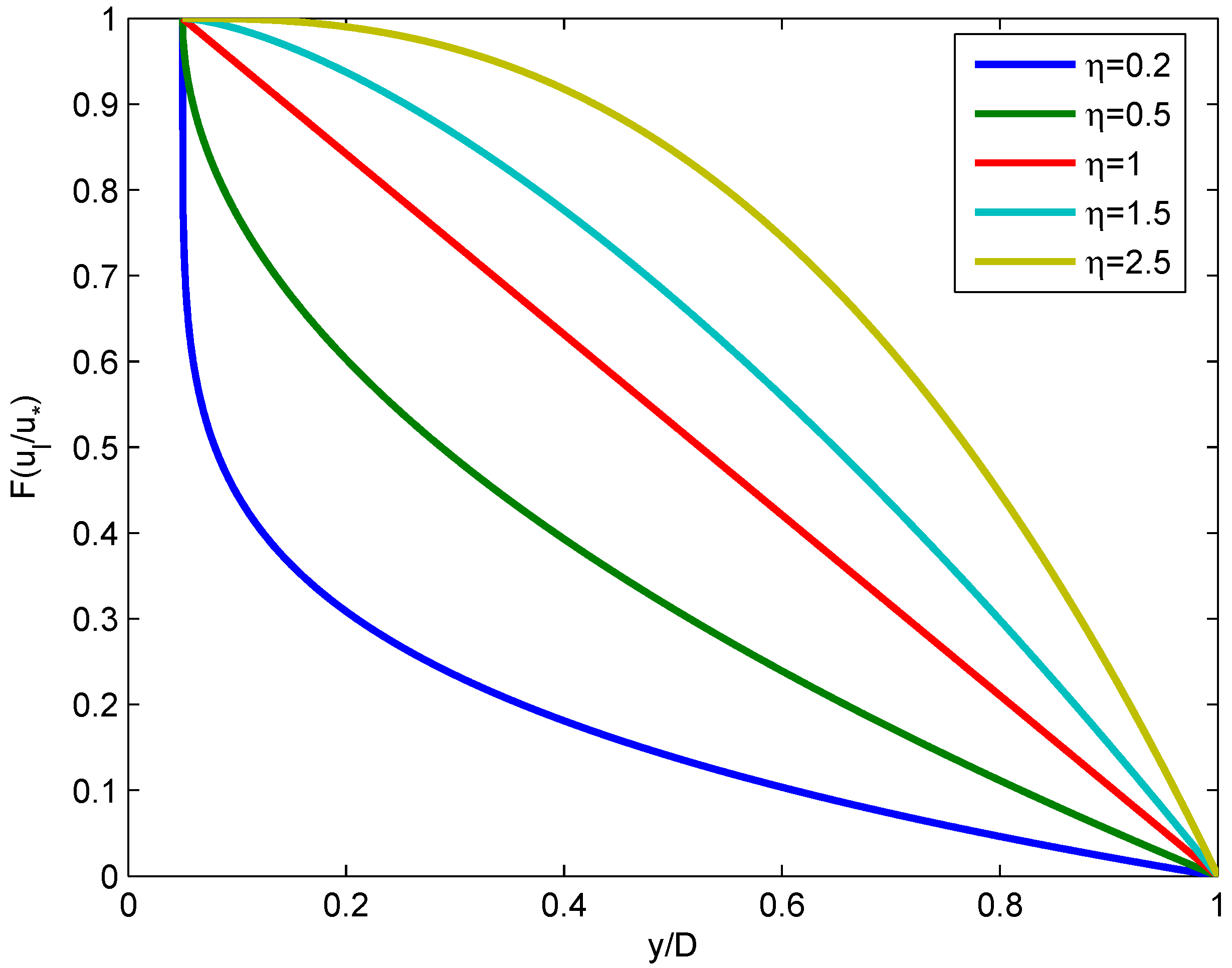
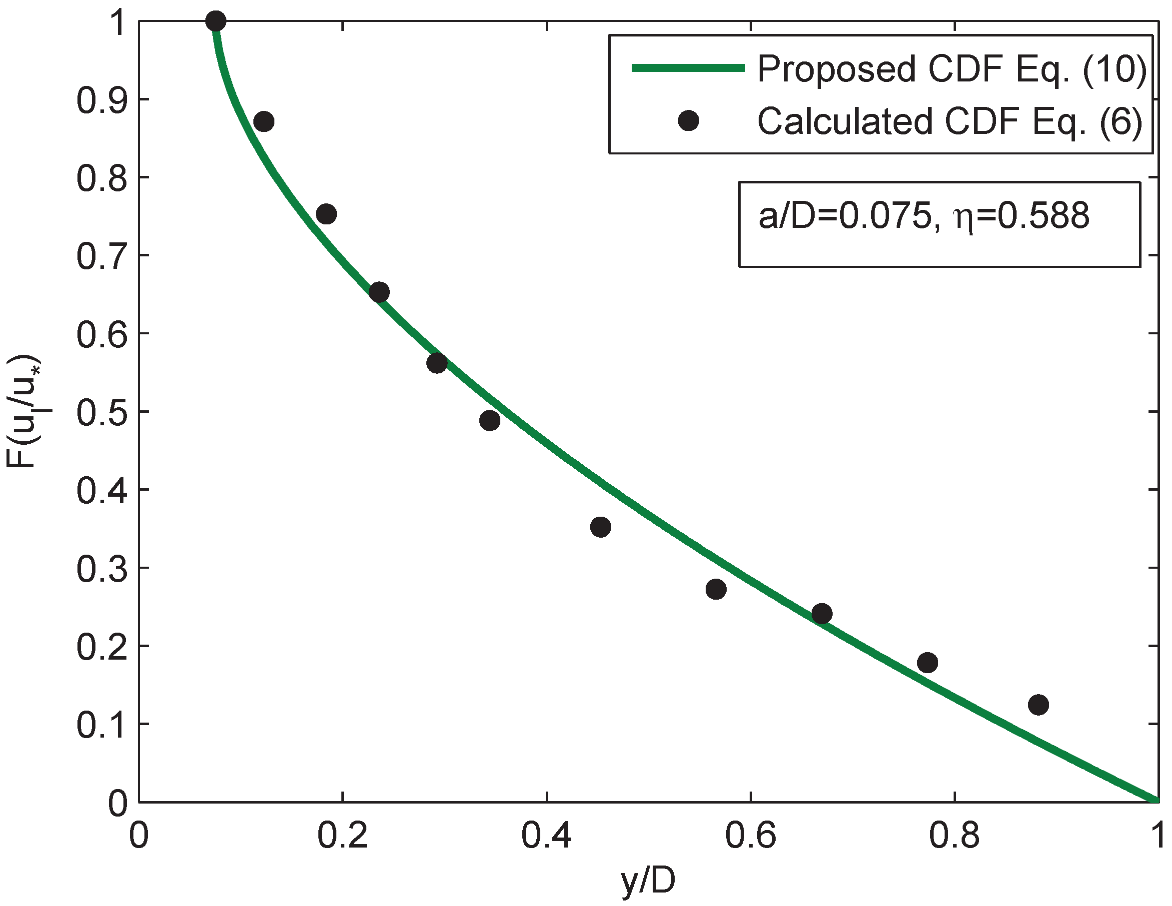
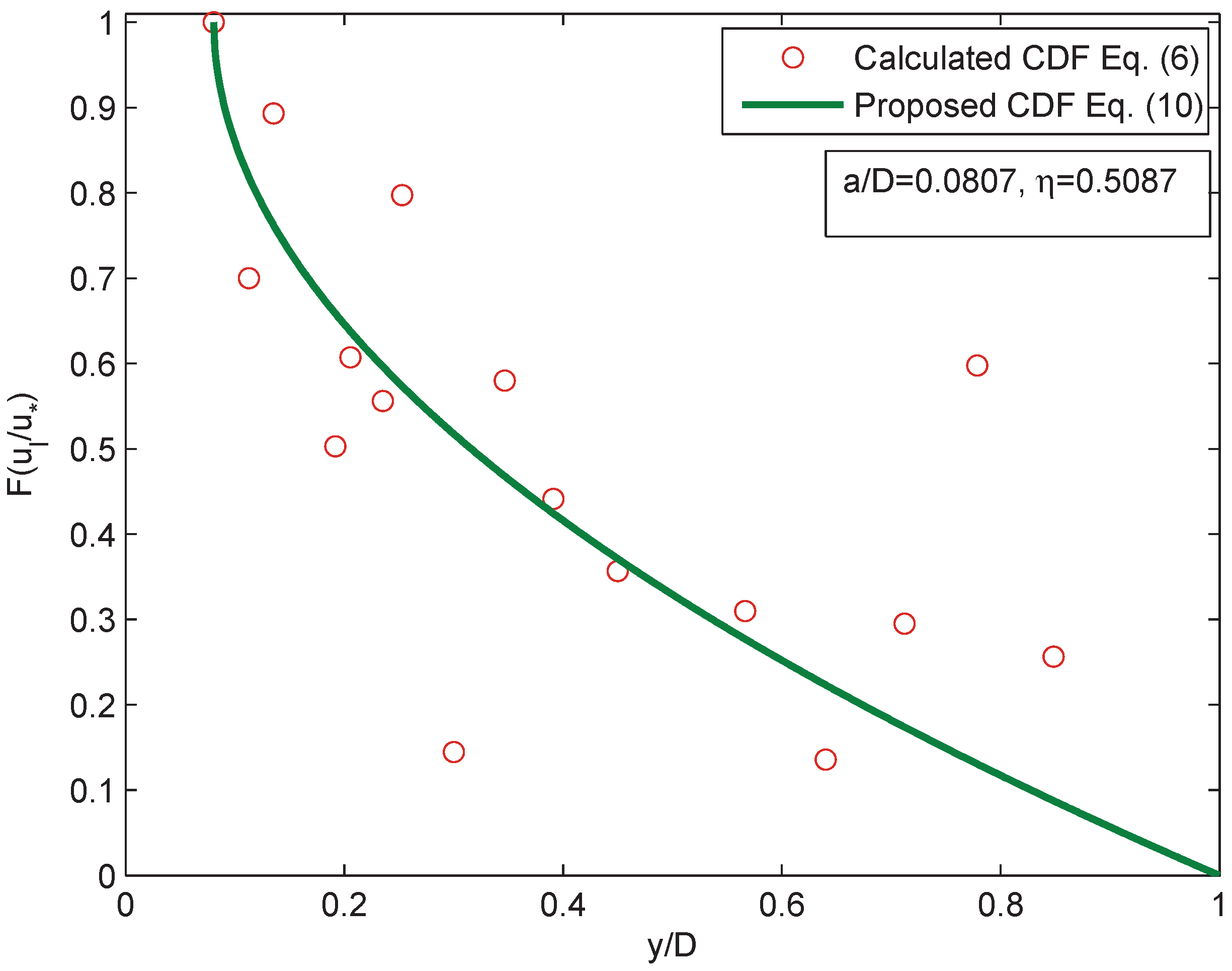
2.5. Cumulative Distribution Function

In order to express the velocity lag in the real (space) domain, an equation connecting the probability domain to the space domain is needed. Therefore, a hypothesis on the CDF of u l ^ in terms of flow depth was formulated as follows:
F ( u l ^ ) = 1 y a D a η
where D is the maximum depth, a is the reference level, y is the vertical height from the channel bed having a range from a to D and η is a fitting parameter. This hypothesis on the CDF is based on two important assumptions: (1) all of the values of y between a and D are equally likely; and (2) the velocity lag increases monotonically from the water surface to the reference level. Exponent η in Equation (10) represents the shape parameter and declination of the CDF. The declination of the proposed CDF curve with the change of exponent η is shown in Figure 1 from which it can be seen that the CDF is linear for η = 1 and is non-linear for other values of η. It is also observed that at a fixed height from the bed, the value of CDF increases with the increase of parameter η. The proposed CDF was validated with the experimental data R1 of Rashidi et al. [4] and SL01 of Muste and Patel [2], presented in Figure 2 and Figure 3, respectively. Despite the fact that there is the zigzag nature of the experimental results of velocity lag, the proposed model CDF in Equation (10) agrees well with the values of CDF computed from Equation (6).

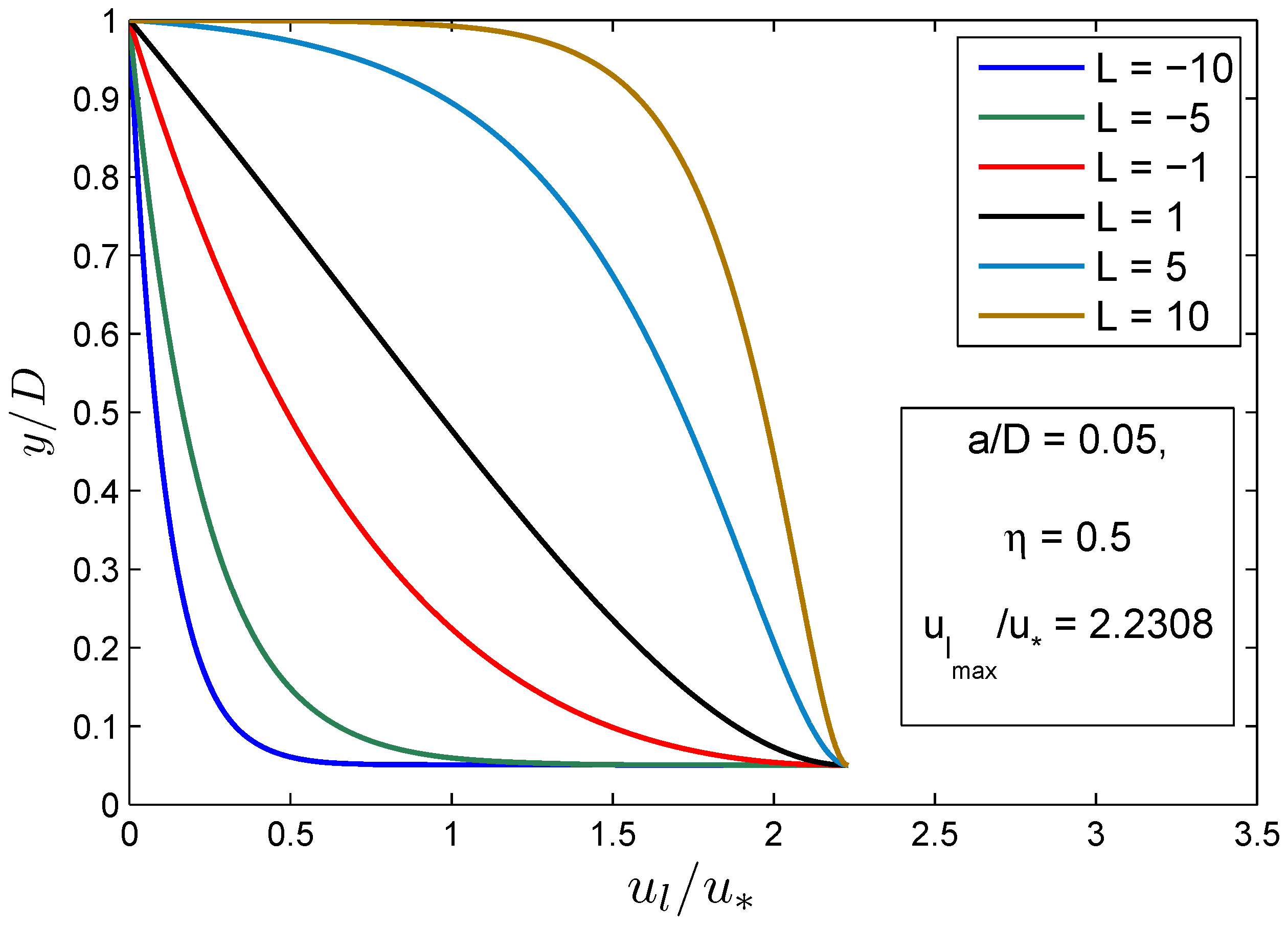
2.6. Derivation of Velocity Lag

Substituting Equation (8) into Equation (6) and equating with Equation (10), we obtain the dimensionless velocity lag of a particle in sediment-laden flow as:
u l u * = 1 λ 1 ln 1 + ( e x p ( λ 1 u ^ l m a x ) 1 ) 1 y a D a η
The velocity lag of a particle moving in a sediment mixed fluid can be calculated from Equation (11) at any height y from the channel bed. It can be observed from Equation (11) that it contains the only unknown parameter λ 1 , which can be obtained by solving non-linear Equations (8) and (9).

2.7. Re-Parametrization

To represent the proposed model in a simple-to-use form, a dimensionless parameter L was introduced here as the entropy parameter. The parameter L was defined as:
L = λ 1 u ^ l m a x
Substituting Equation (12) into Equation (11), the velocity lag equation can be written in terms of the parameter L as:
u l u * = u ^ l m a x L ln 1 + ( e x p ( L ) 1 ) 1 y a D a η
The variation of the velocity lag with the change of entropy parameter L is shown in Figure 4 for fixed values of the parameters a / D = 0.05 , η = 0.5 and u l m a x / u * = 2.23 . The values of these parameters were taken from the experimental observation of run R1 of Rashidi et al. [4]. Figure 4 shows that a change in the L value changes the declination of the velocity lag profile. Furthermore, it can be observed that at a fixed height from the channel bed, the velocity lag of a particle increases with the increase of parameter L.
In a similar manner, the dimensionless entropy function H given in Equation (7) can be expressed in terms of the parameter L as:
H = ln u l ^ m a x ( e x p ( L ) 1 ) L e x p ( L ) ( L 1 ) + 1 e x p ( L ) 1
In Figure 5, the variation of entropy H with parameter L is plotted for the range of L from 10 to 10. From the figure, it is found that the entropy value increases when L increases from 10 to zero, and then, entropy decreases when L further increases from zero to 10. It is also observed from Figure 5 that the curve is symmetrical about the vertical axis. In the range of L from zero to 10, it is observed that the maximum value of entropy occurs when L is close to zero, and with the increase of L, entropy decreases. Thus, parameter L, as an index of velocity lag, gives the entropy value for the distribution. This means that the probability distribution will have more uniformity for smaller L values than for larger L values. Furthermore, the probability density function can be expressed in terms of parameter L from Equations (5) and (8) as:
f ( u l ^ ) = λ 1 exp ( λ 1 u ^ l ) e x p ( L ) 1 = L exp u ^ l / u ^ l m a x u ^ l m a x ( e x p ( L ) 1 )
From Equation (15), we have:
f ( 0 ) f ( u ^ l m a x ) = 1 e x p ( L )
Equation (16) shows that if L = 0 , f ( 0 ) = f ( u ^ l m a x ) , and therefore, the probability density function would tend to be uniform. As the value of L increases, the denominator becomes larger, f ( u ^ l m a x ) tends to infinity and the probability density function becomes non-uniform.
It can be observed from Equation (13) that to find the velocity lag, the determination of entropy parameter L and, hence, the determination of Lagrange multiplier λ 1 are needed, which can be achieved by solving the system of non-linear Equations (2) and (3). Here, we present a graphical method to determine the L value, which is related to u l m e a n / u l m a x . Simple algebraic calculation of Equations (2) and (3) gives the following equation as:
u l m e a n u l m a x = e x p ( L ) e x p ( L ) 1 1 L
Equation (17) shows that the value of parameter L can be determined for given values of u l m e a n , u l m a x without solving the system of non-linear equations. Variation of the u l m e a n / u l m a x with L is presented in Figure 6, which shows that the ratio of mean and maximum velocity lags continuously increase with the increase of entropy parameter L.

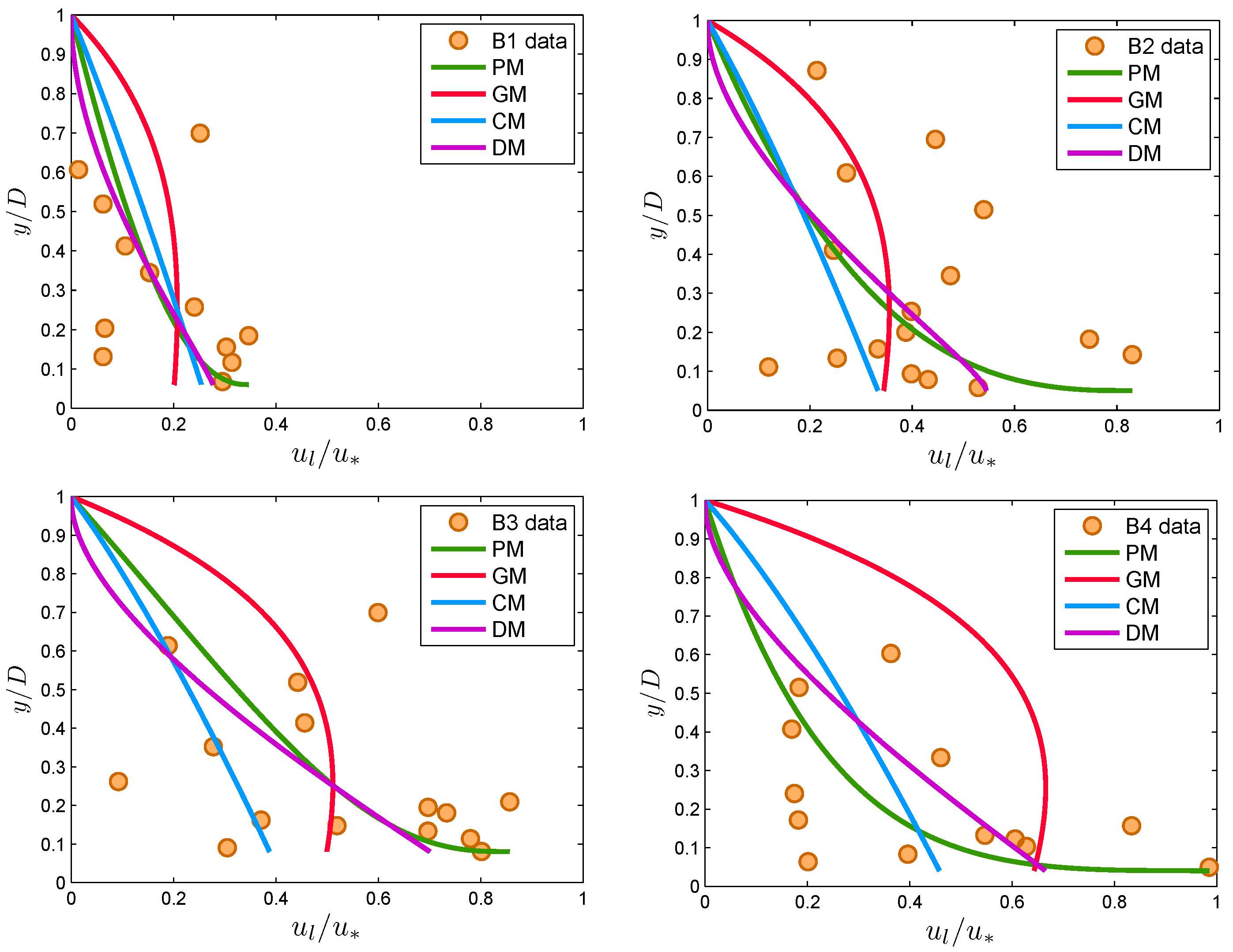
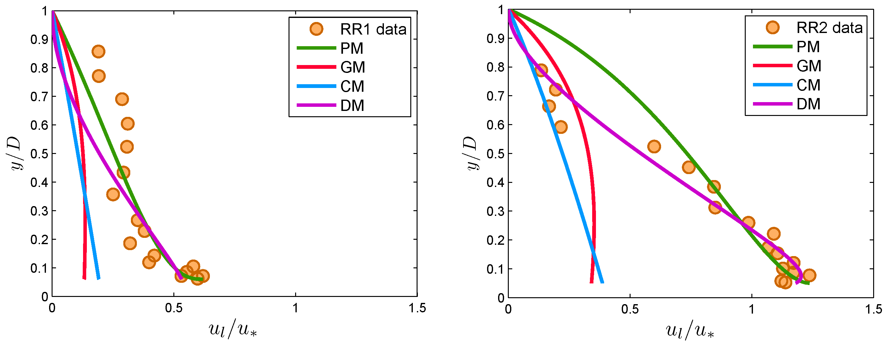
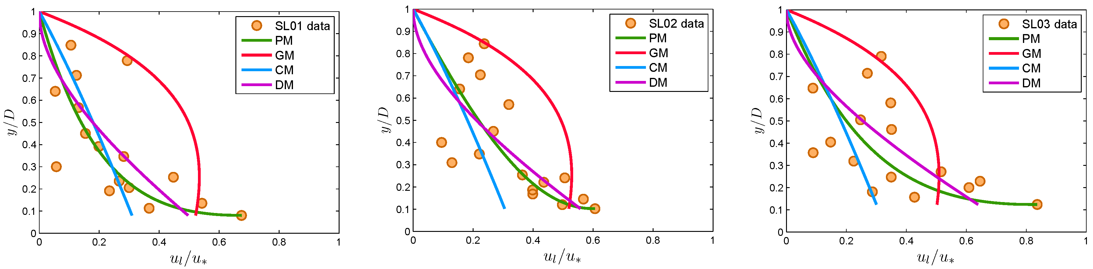
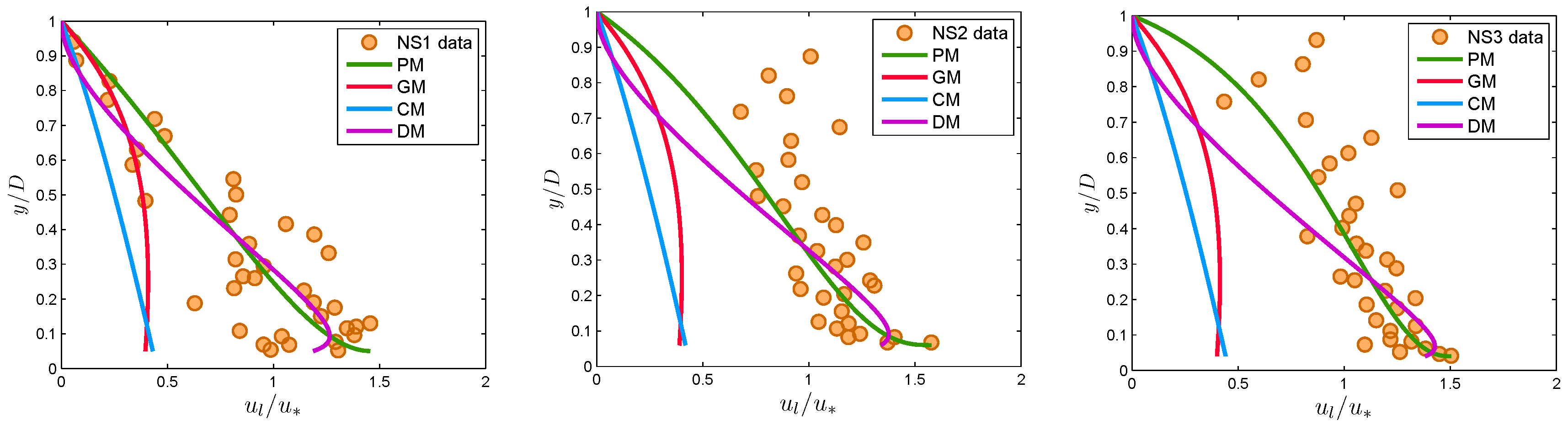
3. Comparison with Experimental Data and Other Models

The proposed model of velocity lag, based on the entropy theory, was validated with experimental observations available in the literature. To test the validity of this model, i.e., Equation (13) with a wide range of sediment-laden flow conditions and different types of particles, experimental data from Rashidi et al. [4] and Kaftori et al. [31] for polystyrene particles, Best et al. [3] and Righetti and Romano [26] for glass particles and Muste and Patel [2] and Muste et al. [32] for natural sand particles were selected. A summary of these data with flow conditions and other flow characteristics is given in Table 1. We can find from the table that the flow parameters vary for a broad range in these experimental runs. We calculated averaged Reynolds number R e A ( = U m d p / ν f ) where U m is the mean flow velocity of sediment-laden fluid over the flow depth, ν f is the kinematic viscosity of fluid and d p denotes the particle diameter. Shields parameter θ (= u * 2 / ( s 1 ) g d p ) is presented in the table, where g is the gravitational acceleration, and s denotes the specific gravity of particles. Table 1 shows the reasonable ranges of the R e A and θ values. Therefore, the present study considered a wide range of experimental runs for verification of the velocity lag model.
The proposed model was also compared with other existing models reported in the literature. The models of velocity lag selected were the models of Cheng [12], Greimann et al. [10] and Pal et al. [13]. These models are deterministic. The Cheng [12] model can be expressed as:
u l u * = 2 2 y D 1 / 1.5 + 1 4 32 ν f u * d p 2 / 1.5 1 2 32 ν f u * d p 1 / 1.5 1.5
Similarly, the model of Greimann et al. [10] can be expressed as:
u l u * = 0.66 ω p u * 1 y D exp 1.34 y D
and the model of Pal et al. [13] can be given as:
u l u * = M A 2 1 / 1.75 + 1 4 N A 2 2 / 1.75 1 2 N A 2 1 / 1.75 1.75
where A 2 = 1.17 and M and N are given by:
M = 2 τ a ρ m u * 2
and:
N = 32.2 μ r ( 1 c ) Δ p ν f u * d p
in which:
τ a = a τ ρ f u * 2 d p y 1 A 3 + A 4 + 1 y D ( 1 c 1 / 3 ) d y
A 3 = ( Δ p + 1 ) c 2 / 3 ( 1 c 1 / 3 ) 2 d p 2 κ m 2 y + Π π D sin π y D 2
A 4 = μ r c 2 / 3 ( 1 c 1 / 3 ) ν f u * κ m y + Π π D sin π y D
Using regression, they proposed the value of a τ as:
a τ = 618.741   Δ p + 1 2.45 u * ω p 0.812 d p D 1.896
where ρ s , ρ f and ρ m are the mass densities of fluid, particle and sediment-fluid mixture, respectively. μ r ( = μ m μ f ) is the relative viscosity, in which μ m and μ f are the dynamic viscosities of sediment-laden and sediment-free fluid, respectively; c denotes the sediment concentration by volume; Δ p + 1 ( = ρ s / ρ f = s ) denotes the specific gravity of particles; ω p is the settling velocity of sediment particles; and κ m denotes the von Karman coefficient of mixture. For the purposes of discussion of the model comparison, the models proposed in the present study and by Cheng [12], Greimann et al. [10] and Pal et al. [13] were denoted, respectively, as PM, CM, GM and DM. Hence, onwards, throughout the present study, we use these acronyms to refer to the corresponding models on velocity lag.
Figure 7 and Figure 8 compare the proposed model Equation (13) with the experimental data of Rashidi et al. [4] and Kaftori et al. [31] for polystyrene particles, respectively. The model parameters were computed as follows: exponent η was obtained after fitting the CDF in Equation (10) to the experimental data; the value of L was computed from Equation (12) after computing the Lagrange multiplier λ 1 by solving the non-linear equations given in Equations (8) and (9). In Figure 7 and Figure 8, the models of CM, GM and DM are also shown for comparison. It can be observed from Figure 7 that the proposed model showed a good agreement with experimental data, whereas models CM, GM and DM underestimated the experimental results over the whole flow depth. Despite the scattered nature of the data, in Figure 8, the present model also showed a favorably good agreement with the experimental data. It can be observed from Figure 8 that the results of PM and DM are comparable to each other. To get a quantitative idea about the goodness of fit, the root-mean-square error was computed, as discussed in the next section.
To test the proposed model for glass particles, the computed values of velocity lag were compared with the observed data of Best et al. [3] and Righetti and Romano [26]. In all cases, the model parameters were computed as mentioned earlier. Figure 9 compares the Best et al. [3] data, and Figure 10 shows the Righetti and Romano [26] data. From Figure 9, it can be seen that all theoretical models gave almost similar results. This indicates that the adoption of an entropy-based approach for modeling velocity lag between fluid and particles in sediment-laden flow is reasonable. It can be seen that PM and DM agreed favorably well with the data, but CM and GM underestimated the velocity lag near the channel bed.
Figure 11 and Figure 12 compare the computed and observed values of velocity lag for natural sand particles with the data from Muste and Patel [2] and Muste et al. [32]. From Figure 11, it is found that PM, CM and DM predicted the results well, but GM overestimated the velocity in all of the test cases, SL01, SL02 and SL03. Figure 12 shows the results due to Muste et al. [32]. It has been found that in run NS1, CM and GM agreed with the observations up to 50% of the flow height from the free surface, but underestimated the lag close to the channel bed; whereas PM and DM predicted well the dataset. In the case of runs NS2 and NS3, the proposed model showed more accurate matching results than did all other models.
It can be seen from the figures that in all of the cases, the entropy-based model derived in the present study dominated over the deterministic models regarding the prediction accuracy of the models. However, entropy-based derivations have some limitations, though not that serious. In this approach, some experimental observations like the u l m a x , u l m e a n values should be known to us in order to compute the Lagrange multipliers. Furthermore, the model behavior depends on the hypothesis of the CDF, which is defined by looking into the flow configuration. In this study, the CDF decreases from the reference level to the water surface, and hence, the derived model of velocity lag also behaves in the same manner. Therefore, the present model can predict those types of experimental observations on velocity lag, which decrease from the reference level to the water surface. This is not only the case for the present model, but also for the other deterministic models with which we are comparing and can be seen from the figures. These discrepancies do not arise due to the theoretical models presented, rather they can be treated as an experimental error commonly found in the experiments related to open channel turbulent flow. Therefore, discrepancies in a few subfigures of Figure 8 and Figure 12 do not prove the weakness of the derived model globally.
Entropy-based derivation does not incorporate explicit fluid mechanics processes; the only physical basis is through the constraints and data. To compute the velocity lag from the proposed model, the unknown parameter η is required, which was computed by fitting the CDF to the experimental data. Now, we try to link the fitting parameter η to some known quantities of flow. For that purpose, a regression analysis was carried out. It is noted that the value of η depends on the particle diameter d p , shear velocity u * , settling velocity ω p , flow depth D and specific gravity s of particles. From regression analysis of the fitted values of η, the following formula was obtained:
η = 0.28 1 L 0.192 s 0.602 u * ω p 0.156 d p D 0.194
The fitted values were compared with the values computed from the regression relation, as shown in Figure 13, except for the negative values of parameter L. The value of the coefficient of regression R 2 was obtained as 0.4317. The value is low due to the scatter of data points in the original velocity lag data. To get more accurate results, more velocity lag data are required.
To examine the prediction accuracy of the derived model as compared to the other models considered in this study, an error analysis was carried out. As the experimental data of velocity lag are highly scattered, we needed a suitable error formula. In all of these twenty-two selected datasets, to get an idea about the goodness of fit, the root-mean-square error was computed for all of the models. The root-mean-square error is calculated form the following formula as:
E = 1 N i = 1 N ( u l ^ c ( i ) u l ^ o ( i ) ) 2
where u l ^ c ( i ) and u l ^ o ( i ) are the computed and observed values of the i-th data point of dimensionless velocity lag ( u l / u * ) in a run and N is the total number of data points in that run. For each of the experimental runs, the computed values of E from PM, GM, CH and DM are shown in Table 2, where the asterisk (*) denotes the least error for that run. It is observed from Table 2 that the proposed model provided the least error for twenty test cases out of twenty-two experimental runs considered here. This result shows the superiority of the entropy-based model to the existing deterministic models of Cheng [12], Greimann et al. [10] and Pal et al. [13].

4. Discussion

While comparing with experimental data and other models in Section 3, we observed from Equation (27) that the physical quantities of flow, such as particle diameter d p , specific gravity s and shear velocity u * , play a significant role in the proposed model on velocity lag. Therefore, this section discusses the effect of these parameters on the derived velocity lag model, as well as uncertainty.
To perform this analysis, we arbitrarily choose an experimental run and varied each of the parameters mentioned above by keeping others fixed. Figure 14, Figure 15 and Figure 16 show the effect of particle diameter d p , shear velocity u * and the specific gravity s, respectively, on the velocity lag. It follows from Figure 14 that velocity lag increases with increasing d p . As d p increases, the mass and surface area of a particle increases; thus, the particle accelerates less with the flow velocity, which results in increased u l . Rashidi et al. [4] obtained the same characteristics in their experiment, which can be observed from Figure 7 and Table 1. Again, Figure 15 demonstrates the effect of shear velocity on the velocity lag profile. It is observed from the figure that the velocity lag decreases with increasing u * . The reason is that shear stress increases with the increase of fluid velocity in terms of u * , which leads the particle to follow fluid velocity, and hence, velocity lag u l decreases. This characteristic was also observed in the work of Pal et al. [13]. On the other hand, Figure 16 suggests that the velocity lag decreases with the increase of specific gravity s. This characteristic is also matched with the analysis of Cheng [12]. The aforementioned discussion delineates that our present model on velocity lag, which is based on entropy, is able to describe the characteristics of velocity lag caused by the interaction between particle and fluid in open channel sediment-laden turbulent flow, and hence, the model is also justified.
The maximum entropy H can be obtained from Equation (14). Figure 17 gives the relation between maximum entropy H and dimensionless maximum velocity lag u ^ l m a x . The relation is obtained from regression analysis as:
H u l m a x u * = 0.84 u l m a x u * 1.05
with a coefficient of regression R 2 = 0.9 . Figure 17 shows that the higher the value of the maximum dimensionless velocity lag u ^ l m a x , the higher the value of entropy H; physically larger u ^ l m a x means that more complexity is involved in the flow; hence, more uncertainty can be expected, which is expressed as a linear relation in Equation (29).

5. Conclusions

In this study, the velocity lag between fluid and sediment particles in a sediment-laden flow is modeled using entropy theory. The model is validated with a wide range of twenty-two sets of experimental data published in the literature. The validation results show that the model predicts the velocity lag between particle and fluid well over the whole flow depth of the open-channel in spite of the scattered nature of the data points. Significance and utilization of the present model can be addressed satisfactorily in the area of sediment transport. Apart from the rigorous numerical solution procedures using the two-phase flow approach, the present model can predict velocity lag for a wide range of flow conditions. Furthermore, if the stream-wise velocity profile u of fluid is known, then we can calculate the stream-wise velocity profile u p of particles without any difficulty. The model is also compared with three existing models. To measure the accuracy of these models, the root-mean-square error is computed, and it is found that the proposed model gives the best approximation of the velocity lag of particles among the models investigated. The effect of different flow parameters on the derived model of velocity lag is also evaluated. To that end, the model is verified by comparing to the previous models of velocity lag.

Author Contributions

All authors contributed extensively to the work presented in this paper. Manotosh Kumbhakar and Koeli Ghoshal had the original idea of this study. Snehasis Kundu and Manotosh Kumbhakar formulated the model and discussed the analysis of the study. Vijay P. Singh and Koeli Ghoshal made editing corrections and improvements to the manuscript. All authors have read and approved the final manuscript.

Conflicts of Interest

The authors declare no conflict of interest.

References

  1. Bagnold, R.A. The nature of saltation and bedload transport in water. Proc. R. Soc. Lond. Ser. A 1973, 332, 473–504. [Google Scholar] [CrossRef]
  2. Muste, M.; Patel, V.C. Velocity profiles for particles and liquid in open-channel flow with suspended sediment. J. Hydraul. Eng. 1997, 123, 742–751. [Google Scholar] [CrossRef]
  3. Best, J.; Bennett, S.; Bridge, J.; Leeder, M. Turbulence modulation and particle velocities over flat sand beds at low transport rates. J. Hydraul. Eng. 1997, 123, 1118–1129. [Google Scholar] [CrossRef]
  4. Rashidi, M.; Hetsroni, G.; Banerjee, S. Particle-turbulence interaction in a boundary layer. Int. J. Multiph. Flow 1990, 16, 935–949. [Google Scholar] [CrossRef]
  5. Taniere, A.; Oesterle, B.; Monnier, J.C. On the behavior of solid particles in a horizontal boundary layer with turbulence and saltation effects. Exp. Fluids 1997, 23, 463–471. [Google Scholar]
  6. Kiger, K.T.; Pan, C. Suspension and turbulence modification effects of solid particulates on a horizontal turbulent channel flow. J. Turbul. 2002. [Google Scholar] [CrossRef]
  7. Chauchat, J.; Guillou, S. On turbulence closures for two-phase sediment-laden flow models. J. Geophys. Res. Oceans 2008. [Google Scholar] [CrossRef]
  8. Bombardelli, F.A.; Jha, S.K. Hierarchical modeling of the dilute transport of suspended sediment in open channels. Environ. Fluid Mech. 2009, 9, 207–235. [Google Scholar] [CrossRef]
  9. Jha, S.K.; Bombardelli, F.A. Toward two-phase flow modeling of nondilute sediment transport in open channels. J. Geophys. Res. 2010, 115. [Google Scholar] [CrossRef]
  10. Greimann, B.P.; Muste, M.; Holly, F.M. Two-phase formulation of suspended sediment transport. J. Hydraul. Res. 1999, 37, 479–500. [Google Scholar] [CrossRef]
  11. Jiang, J.S.; Law, A.W.K.; Cheng, N.S. Two-phase modeling of suspended sediment distribution in open channel flows. J. Hydraul. Res. 2004, 42, 273–281. [Google Scholar] [CrossRef]
  12. Cheng, N.S. Analysis of velocity lag in sediment-laden open channel flows. J. Hydraul. Eng. 2004, 130, 657–666. [Google Scholar] [CrossRef]
  13. Pal, D.; Jha, S.K.; Ghoshal, K. Velocity lag between particle and liquid in sediment-laden open channel turbulent flow. Eur. J. Mech. B Fluids 2016, 56, 130–142. [Google Scholar] [CrossRef]
  14. Vowinckel, B.; Kempe, T.; Fröhlich, J. Fluid–particle interaction in turbulent open channel flow with fully-resolved mobile beds. Adv. Water Resour. 2014, 72, 32–44. [Google Scholar] [CrossRef]
  15. Shao, X.; Wu, T.; Yu, Z. Fully resolved numerical simulation of particle-laden turbulent flow in a horizontal channel at a low Reynolds number. J. Fluid Mech. 2012, 693, 319–344. [Google Scholar] [CrossRef]
  16. Derksen, J.J. Simulations of granular bed erosion due to a mildly turbulent shear flow. J. Hydraul. Res. 2015, 53, 622–632. [Google Scholar] [CrossRef]
  17. Finn, J.R.; Li, M. Regimes of sediment-turbulence interaction and guidelines for simulating the multiphase bottom boundary layer. Int. J. Multiph. Flow 2016, 85, 278–283. [Google Scholar] [CrossRef]
  18. Chiu, C.L. Entropy and probability concepts in hydraulics. J. Hydraul. Eng. 1987, 113, 583–600. [Google Scholar] [CrossRef]
  19. Cui, H.; Singh, V.P. Two-dimensional velocity distribution in open channels using the Tsallis entropy. J. Hydrol. Eng. 2012, 18, 331–339. [Google Scholar] [CrossRef]
  20. Cui, H.; Singh, V.P. One-dimensional velocity distribution in open channels using Tsallis entropy. J. Hydrol. Eng. 2013, 19, 290–298. [Google Scholar] [CrossRef]
  21. Kumbhakar, M.; Ghoshal, K. One-Dimensional velocity distribution in open channels using Renyi entropy. Stoch. Environ. Res. Risk Assess. 2016. [Google Scholar] [CrossRef]
  22. Kumbhakar, M.; Ghoshal, K. Two dimensional velocity distribution in open channels using Renyi entropy. Phys. A Stat. Mech. Appl. 2016, 450, 546–559. [Google Scholar] [CrossRef]
  23. Chiu, C.; Jin, W.; Chen, Y. Mathematical models for distribution of sediment concentration. J. Hydraul. Eng. 2000, 126, 16–23. [Google Scholar] [CrossRef]
  24. Cui, H.; Singh, V.P. Suspended sediment concentration in open channels using Tsallis entropy. J. Hydrol. Eng. 2013, 19, 966–977. [Google Scholar] [CrossRef]
  25. Singh, V.P.; Cui, H. Modeling sediment concentration in debris flow by Tsallis entropy. Phys. A Stat. Mech. Appl. 2015, 420, 49–58. [Google Scholar] [CrossRef]
  26. Righetti, M.; Romano, G.P. Particle-fluid interactions in a plane near-wall turbulent flow. J. Fluid Mech. 2004, 505, 93–121. [Google Scholar] [CrossRef]
  27. Shannon, C.E. The mathematical theory of communications, I and II. Bell Syst. Tech. J. 1948, 27, 379–423. [Google Scholar] [CrossRef]
  28. Jaynes, E. Information theory and statistical mechanics: I. Phys. Rev. 1957, 106, 620–930. [Google Scholar] [CrossRef]
  29. Jaynes, E. Information theory and statistical mechanics: II. Phys. Rev. 1957, 108, 171–190. [Google Scholar] [CrossRef]
  30. Jaynes, E. On the rationale of maximum entropy methods. Proc. IEEE 1982, 70, 939–952. [Google Scholar] [CrossRef]
  31. Kaftori, D.; Hetsroni, G.; Banerjee, S. Particle behavior in the turbulent boundary layer velocity and distribution profiles. Phys. Fluids 1995, 7, 1107–1121. [Google Scholar] [CrossRef]
  32. Muste, M.; Yu, K.; Fujita, I.; Ettema, R. Two-phase versus mixed-flow perspective on suspended sediment transport in turbulent channel flows. Water Resour. Res. 2005, 41. [Google Scholar] [CrossRef]
Figure 1. Variation of the proposed CDF with fitting parameter η.
Entropy 18 00318 g001
Figure 2. Validation of the proposed CDF for the R1 data of Rashidi et al. [4].
Entropy 18 00318 g002
Figure 3. Validation of the proposed CDF for the SL01 data of Muste and Patel [2].
Entropy 18 00318 g003
Figure 4. Variation of the velocity lag equation with different L values.
Entropy 18 00318 g004
Figure 5. Variation of the dimensionless entropy with entropy parameter L.
Entropy 18 00318 g005
Figure 6. Ratio of the mean-max velocity lag with entropy parameter L.
Entropy 18 00318 g006
Figure 7. Verification of the proposed model (Equation (13)) with runs R1, R2, R3 and R4 of [4] and the comparison with the models of GM, CM and DM given by Equations (19), (18) and (20).
Entropy 18 00318 g007
Figure 8. Verification of the proposed model (Equation (13)) with runs K11, K12, K13, K21, K22 and K23 of [31] and comparison with the models of Greimann et al. (GM), Cheng (CM) and DM, given by Equations (19), (18) and (20).
Entropy 18 00318 g008
Figure 9. Verification of the proposed model (Equation (13)) with runs B1, B2, B3 and B4 of [3] and the comparison with the models of GM, CM and DM given by Equations (19), (18) and (20).
Entropy 18 00318 g009
Figure 10. Verification of the proposed model (Equation (13)) with runs RR1 and RR2 of [26] and the comparison with the models of GM, CM and DM given by Equations (19), (18) and (20).
Entropy 18 00318 g010
Figure 11. Verification of the proposed model (Equation (13)) with runs SL01, SL02 and SL03 of [2] and the comparison with the models of GM, CM and DM given by Equations (19), (18) and (20).
Entropy 18 00318 g011
Figure 12. Verification of the proposed model (Equation (13)) with runs NS1, NS2 and NS3 of [32] and the comparison with the models of GM, CM and DM given by Equations (19), (18) and (20).
Entropy 18 00318 g012
Figure 13. Comparison between fitted (from Equation (10)) and computed values of η (from Equation (27)).
Entropy 18 00318 g013
Figure 14. Effect of particle diameter on velocity lag.
Entropy 18 00318 g014
Figure 15. Effect of shear velocity on velocity lag.
Entropy 18 00318 g015
Figure 16. Effect of specific gravity on velocity lag.
Entropy 18 00318 g016
Figure 17. Relationship of H ( u ^ l m a x ) with u ^ l m a x .
Entropy 18 00318 g017
Table 1. Summary of the experimental data.
LiteratureRun d p ρ s / ρ f D U m u * ν f R e A Shields
(mm)(cm)(cm/s)(cm/s)(cm 2 /s)Parameter θ
Rashidi et al. [4]R10.1200.032.7515.600.900.008422.30.067
R20.2200.032.7515.600.900.008440.90.036
R30.6500.032.7515.600.900.0084120.90.012
R41.1000.032.7515.600.900.0084204.50.007
Kaftori et al. [31]K110.1000.053.2524.501.280.008030.50.159
K120.2750.053.2724.101.290.007983.50.059
K130.9000.053.2724.851.340.0081276.10.019
K210.1000.053.5231.651.600.008139.20.249
K220.2750.053.5132.101.600.0080110.90.090
K230.9000.053.7729.451.550.0078339.80.026
Best et al. [3]B10.1251.605.7558.003.400.008387.00.363
B20.1751.605.7558.003.400.0083121.80.259
B30.2251.605.7558.003.400.0083156.70.201
B40.2751.605.7558.003.400.0083191.50.165
Righetti and Romano [26]RR10.1001.602.3057.003.290.009063.30.424
RR20.2001.602.0060.003.970.0094127.70.309
Muste and Patel [2]SL010.2301.6512.962.903.020.0103140.50.153
SL020.2301.6512.962.903.050.0103140.50.156
SL030.2301.6512.863.303.130.0105138.70.164
Muste et al. [32]NS10.2301.652.1081.304.200.0093200.40.295
NS20.2301.652.1079.604.200.0096191.70.295
NS30.2301.652.1079.304.200.0091200.20.295
Table 2. Calculation of error E from different models ( * corresponds to minimum error).
LiteratureRunPMGMCMDM
Rashidi et al. [4]R10.0756 * 1.28491.24880.1445
R20.1098 * 1.48481.43960.2132
R30.2266 * 1.90721.97230.6268
R40.2788 * 1.78282.08180.8430
Kaftori et al. [31]K110.4477 * 0.59590.56390.4662
K120.2365 * 0.42140.34580.2495
K130.2105 * 0.69450.74920.2310
K210.2251 * 0.46270.42770.3127
K220.2284 * 0.55250.44110.2908
K230.3263 * 0.65190.60830.3901
Best et al. [3]B10.1023 * 0.11390.10390.1049
B20.23180.1938 * 0.24190.2225
B30.2289 * 0.23160.30020.2369
B40.2284 * 0.32720.24170.2345
Righetti and Romano [26]RR10.0745 * 0.29270.26660.1066
RR20.17400.61520.61920.0760 *
Muste and Patel [2]SL010.1043 * 0.26660.14390.1268
SL020.1020 * 0.20340.16120.1201
SL030.1530 * 0.22130.22460.1758
Muste et al. [32]NS10.21660.60700.63780.2103 *
NS20.2505 * 0.73200.78990.3469
NS30.1994 * 0.74480.79540.3469

