1. Introduction
Complex systems are typically characterized by a finite, usually large, number of non-identical interacting entities that often are complex systems themselves, with strategies and autonomous behaviors. Complex system science is a relatively young research area, and it is raising interest among many researchers, mainly thanks to the emerging of new techniques in several fields, such as physics, mathematics, computer science and data analysis [
1].
Complex systems are analyzed using mainly two different approaches: one that provides a global and abstract description by systems of differential equations [
2] and the other that focuses on the interacting components, which are generally simulated by an agent-based model and simulation framework [
3].
In terms of data volume, a complex system can be associated with a big dataset. To extract useful information from these data, new techniques have been recently introduced, most of them in the area of topological data analysis (TDA) [
4]. Topology is the branch of mathematics that studies the connectivity of spaces or, in general, the features of shapes [
5]. TDA is largely used for the analysis of complex systems; for instance, Ibekwe
et al. [
6] used TDA for reconstructing the relationship structure of
Escherichia coli O157, and the authors proved that the non-O157 is in 32 soils (16 organic and 16 conventionally-managed soils). TDA was also used by De Silva [
7] for the analysis of sensor networks, and it was successfully applied to the study of viral evolution in biological complex systems [
8]. Petri
et al. [
9] used a homological approach for studying the characteristics of functional brain networks at the mesoscopic level.
TDA is a new discipline inspired by homology theory [
5]. Informally, homology is a machinery for counting the number of
n-dimensional holes in a topological space. In our approach, we consider only combinatorial objects: simplices (
i.e., vertices, line segments, triangles, tetrahedra, and so on) and simplicial complexes,
i.e., collections of simplices [
5] (see
Figure 1). Simplicial complexes are analyzed via persistent homology, which allows one to identify the generators of persistent
n-dimensional holes [
4,
10].
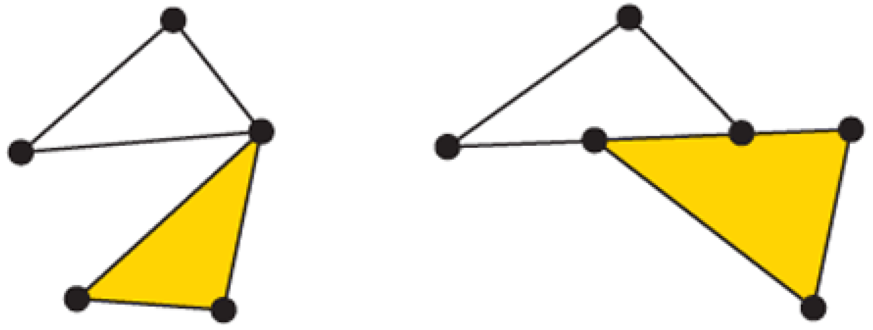
Figure 1.
On the left, a simplicial complex formed by one two-simplex (yellow filled triangle) and three one-simplices (segments forming the non-filled triangle) and three zero-simplices (the vertices). On the right, an invalid simplicial complex; the intersection between the yellow filled triangle and the one-simplex belonging to the upper triangle is not empty, and they do not share a common face.
In this work, we propose a methodology for modeling complex systems that is based on TDA. Our contribution has been inspired by
[
11], a paradigm for modeling complex systems. It was used as a general framework for modeling adaptivity in software systems [
12], but it was conceived for all kinds of complex systems (biological, physical, chemical, and so on).
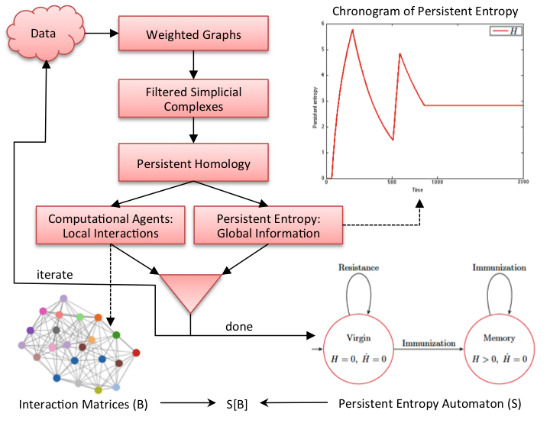
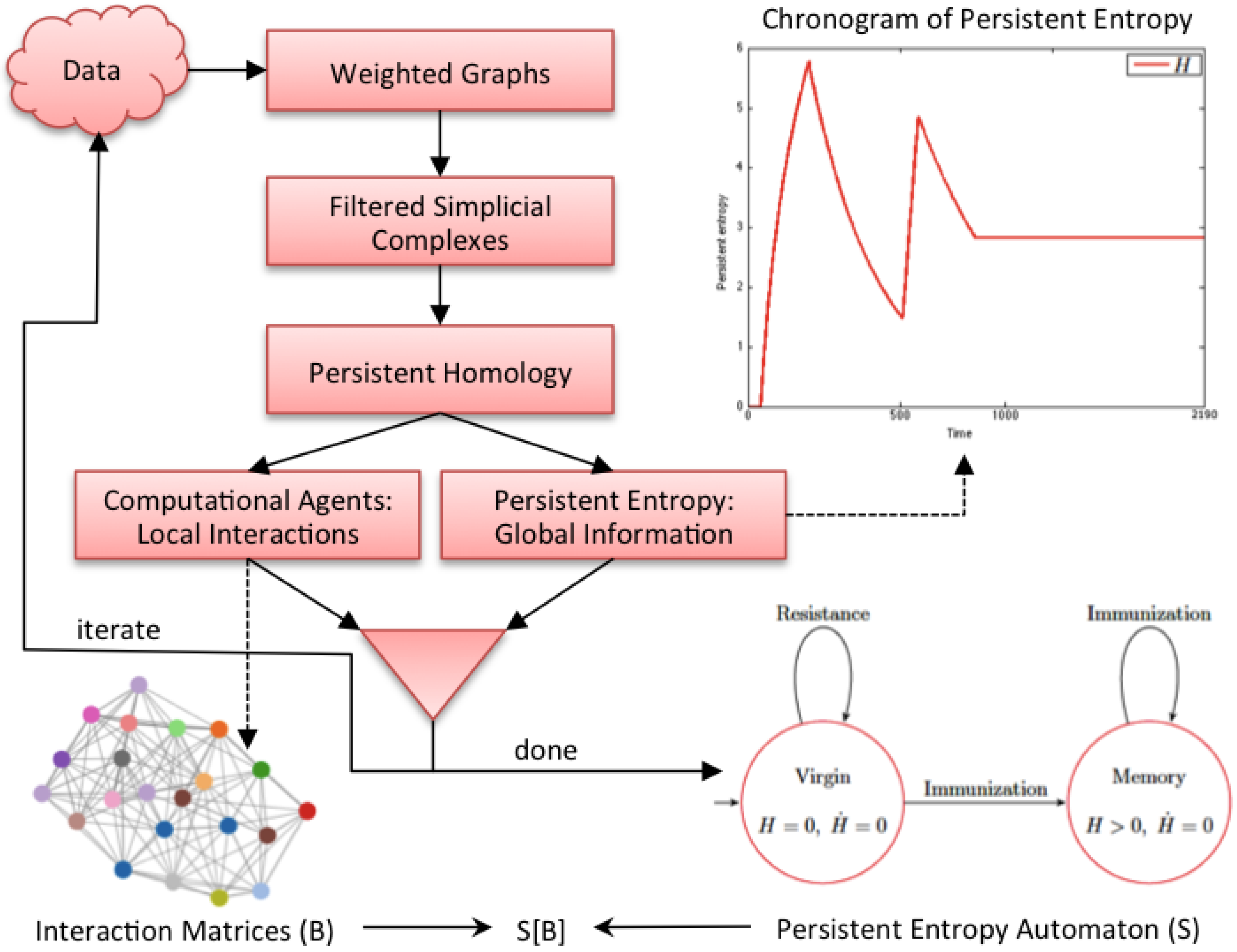
Figure 2 graphically shows our methodology. It is an iterative process where each iteration corresponds to the analysis of a data sample (observation) of the complex system under study. In each iteration, data are first converted into a weighted graph in order to apply the subsequent steps. The graph is taken as the scaffold of the topological space from which the representation with a filtered simplicial complex is derived. Then, persistent homology is computed in order to calculate the topological invariants of the underlying topological space and to identify their generators. At this point, two kinds of information are derived: the computational agents (from the generators) that give rise to the behavioral level
B of
and the persistent entropy (from the invariants) that is a newly-introduced entropic measure describing the global dynamics of the complex system.
Figure 2.
Graphical representation of our methodology. All of the details are explained in the text.
Figure 2.
Graphical representation of our methodology. All of the details are explained in the text.
At the end of the iteration, we construct an model in which the structural level S is a persistent entropy automaton, derived from all of the values of persistent entropy calculated during the iterations. The computational agents identified at each iteration step, formally represented by interaction matrices, are the sequence of B levels associated with the observed evolution of .
To validate our methodology, we consider, as a case study, the idiotypic network (IN) model [
13] of the mammalian immune system. The latter has been largely studied as a complex adaptive system [
14], and several other models are available. Concerning the IN model, we consider the simplified description given by Parisi [
15], and we use the agent-based simulator
C-ImmSim [
16] for generating the data to validate our approach. In this work, we analyzed simulated data instead of real data in order to validate the correctness of the methodology in a more controlled way.
The paper is organized as follows.
Section 2 introduces the case study of the IN.
Section 3 describes our methodology step by step in order to extract from that data a two-level model according to the
paradigm. In
Section 4, the methodology is applied to the case study of IN, and finally,
Section 5 provides concluding remarks.
2. Case Study
In this paper, we illustrate the steps of the proposed methodology applied to a case study in a biological immune system, specifically to the immune network theory by Nielse Jerne [
13]. Jerne theorized that the immune system can be thought of as a regulated network of antibodies and anti-antibodies, called the idiotypic network. Let us briefly recall the main mechanisms described by the model. When an antigen is presented to the organism, the immune system reacts in the following two ways: innate immunity and adaptive (or acquired) immunity. Innate immune defenses are non-specific, meaning that these systems respond to pathogens in a generic way. The innate immune system is the dominant system of the host defense in most organisms; it involves the epithelial barriers, the phagocytes, the dendritic cells, the plasma proteins and the NK cells. The adaptive immune system, on the other hand, is called into action against pathogens that are able to evade or overcome innate immune defenses. The first reaction of the immune system is governed by the mechanism of the innate immunity, and its lifespan is up to 12 h; after that period, in the case of the presence of antigens, the adaptive response is triggered. The adaptive immune system is mainly composed of B cells, antibodies, naive T cells and effector T cells. When activated, these components adapt to the presence of infectious agents by activating, proliferating and creating potent mechanisms for neutralizing or eliminating the antigens. The lifespan of the adaptive response depends on the type of infection. In this work, we are interested in studying the behavior of the antibodies involved during the adaptive response, and we present a general example of this scenario. Suppose an antigen is recognized by B cells, which secrete antibodies, say
.
themselves are then recognized as anti-antibodies by anti-idiotypic B cells, which secrete other antibodies, say
. Thus, further interactions lead to
antibodies that recognize the
ones, and so on.
In an IN, there is no intrinsic difference between an antigen and an antibody. Moreover, any node of the network can bind to and be bound to any other antigen or antibody. This phenomenon is known as the idiotypic cascade. During the ontogenesis phase, the immune system learns which antibodies should not be produced, and the system remembers these decisions for its entire life. This phenomenon is called immunological memory. The important properties of this system, including memory, are then the properties of the network of cells as a whole, rather than of the individual cells [
17]. The IN model has been used by Parisi [
15] to derive a simplified model for describing the dynamics of a functional network of antibodies in the absence of antigens. The dynamics
of each antibody
i (
) at equilibrium is simply described by Equation (
1):
where
represents the influence of antibody
k on antibody
i. If
is positive, antibody
k triggers the production of antibody
i, whereas if
is negative, antibody
k suppresses the production of antibody
i.
is a measure of the efficiency of the control of antibody
k on antibody
i. The values of
are distributed in the interval
.
is a threshold parameter that regulates the dynamics when the couplings
are all very small; otherwise, one can assume
equal to zero. The concentration
of antibody
i is assumed to have, in absence of external antigens, only two values, conventionally zero or one (in the presence of antigen concentrations,
might become
). The immune system state is determined by the values of all
’s for all possible antibodies
.
represents the total stimulatory/inhibitory effect (depending on its sign) of the whole network on the
i-th antibody.
is positive when the excitatory effect of the other antibodies is greater than the suppressive effect; otherwise,
is negative.
3. Methodology
The aim of our methodology is to extract, applying TDA, local and global information from a dataset. In particular, the output of the methodology is a set of models specified within the
paradigm [
11]. In the
paradigm, a model has two levels of description, namely the
S global or structural level and the
B local or behavioral level, which are entangled in order to express the behavior of the system as a whole. The
S level describes how the system evolves following global information coming from the environment in which it is operating and from the interactions and the evolutions of the entities of the
B level. Note that this approach has some similarities to hierarchical models like the hierarchical automata proposed by Mikk
et al. [
18]. However, in our case, the levels cannot be seen as just different levels of abstraction, but they can exist only in the entangled
model.
3.1. From Data to Weighted Graphs
We start from data that comes from observations, over time, of the complex system under study. The first step to be accomplished is to represent such data as weighted graphs where:
nodes represent the interacting components;
an edge, equipped with a weight, expresses an interaction (or a distance) between two components.
Note that this step is always possible because the weight can be defined using statistical descriptors (correlation coefficients, scoring systems, and so on), metric functions (normalized Euclidean distance, Hamming distance, and so on) or domain-dependent features.
3.2. From Weighted Graphs to Filtered Simplicial Complexes
In this work, we are interested in filtering simplicial complexes for studying the connectivity among the entities belonging to a complex system. The data space can be represented by simplicial complexes, which are combinatorial objects. From a geometrical point of view, a simplicial complex is obtained by properly gluing together smaller components, the so-called simplices. Low dimensional simplices are:
- -
0-simplex, geometrically represented by a vertex;
- -
1-simplex, geometrically represented by an edge;
- -
2-simplex, geometrically represented by a filled triangle;
- -
3-simplex, geometrically represented by a filled tetrahedron formed by filled triangles;
- -
⋯
In order to build a simplicial complex, the intersection between two simplices must be empty or they must have in common at least one face (see
Figure 1). Graphs are strictly related to the representation of topological spaces; in particular, a graph can be viewed as a simplicial complex obtained by gluing together 0-simplices through 1-simplices.
Given a directed or undirected graph, it is possible to construct from it a simplicial complex following several approaches [
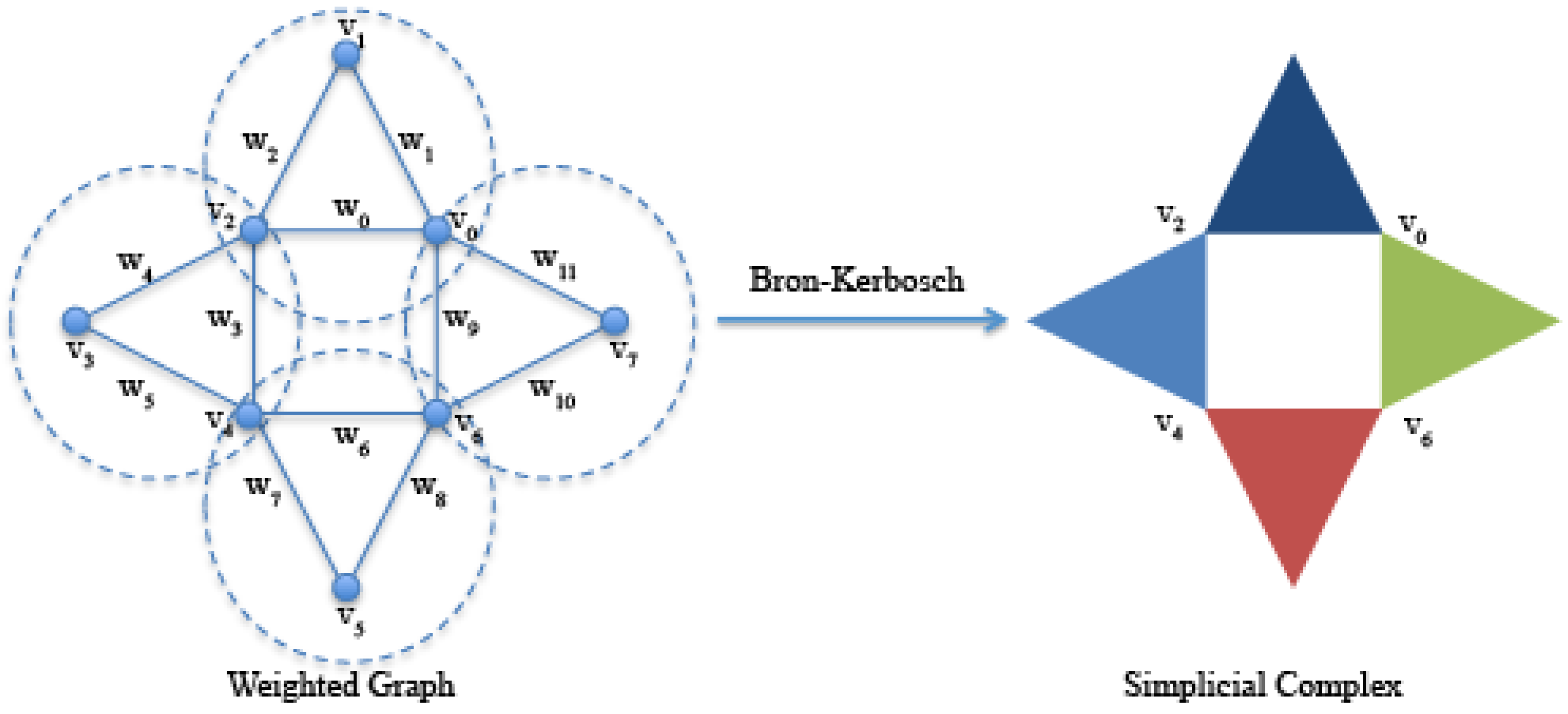
19]. In this work, we use the clique complexes; given a graph
, a clique is a complete subgraph, and a maximal clique is a clique that is not contained in a larger clique. We use the Bron–Kerbosch algorithm [
20] for listing all of the maximal cliques of a graph. As shown in
Figure 3, a simplicial clique complex of
G is the simplicial complex whose simplices are all of the maximal cliques of
G. Since a
k-clique is equivalent to a
-simplicial complex, then a 3-clique is equivalent to a 2-simplicial complex, and so on [
21].
Figure 3.
On the left, an undirected graph formed by eight vertices and twelve edges with weights with . Highlighted by dashed circles, the four 3-maximal cliques , , and identified by the Bron–Kerbosch algorithm. On the right, the simplicial complex formed by the four 2-simplices (filled triangles) corresponding to the four 3-maximal cliques.
The computational algorithms for the characterization of simplicial complexes require as input a filtered simplicial complex,
i.e., a simplicial complex equipped with a filter value. A filter value [
22] can be considered as a time-appearing value along the process described below. The set of obtained filter values is called the filter set and must be a strictly ordered set. The general algorithm for building a filtered simplicial clique complex from a weighted graph is described as follows:
list all maximal cliques of G with the Bron–Kerbosch algorithm;
for each maximal clique, select the minimum (or the maximum) value of the weights of its edges;
for each maximal clique, assign the value selected in Equation (2) to the corresponding simplicial complex as the filter value.
Figure 4.
On the right, the filtered simplicial complex derived from the algorithm where the filter values are selected as the minimum of the weights. As a result, we set , because we want a filter set , such that .
Figure 4.
On the right, the filtered simplicial complex derived from the algorithm where the filter values are selected as the minimum of the weights. As a result, we set , because we want a filter set , such that .
3.3. Computation of Persistent Homology on Filtered Simplicial Complexes
Topological spaces can be characterized by using topological invariants. In this work, we use simplicial complexes as topological spaces and persistent homology to determine their invariants [
5]. Persistent homology is the computational implementation of homology, which allows one to describe a simplicial complex in terms of
n-dimensional holes. These quantities are expressed by the Betti numbers
, where
, described as follows:
- -
corresponds to the number of connected components;
- -
corresponds to the number of planar holes;
- -
corresponds to the number of voids in solid objects (2-dimensional holes);
- -
…
Moreover, for Betti numbers
, a set
of generators of the corresponding topological features can be identified. Such generators are the simplices involved in the formation of the
i-dimensional holes. Elements of
will be denoted by
to identify 0-simplices; elements of
will be denoted by edges
; elements of
are (filled) triangles denoted by
, and so on [
5].
Basically, persistent homology is an incremental construction of the final filtered simplicial complex. The clique weight rank persistent homology algorithm (CWRPH) [
23] is used, which has been efficiently implemented by the tool jHoles [
24]. At each step of the algorithm, the family of simplices associated with the current filter value are introduced into the topological space, and the Betti numbers are computed.
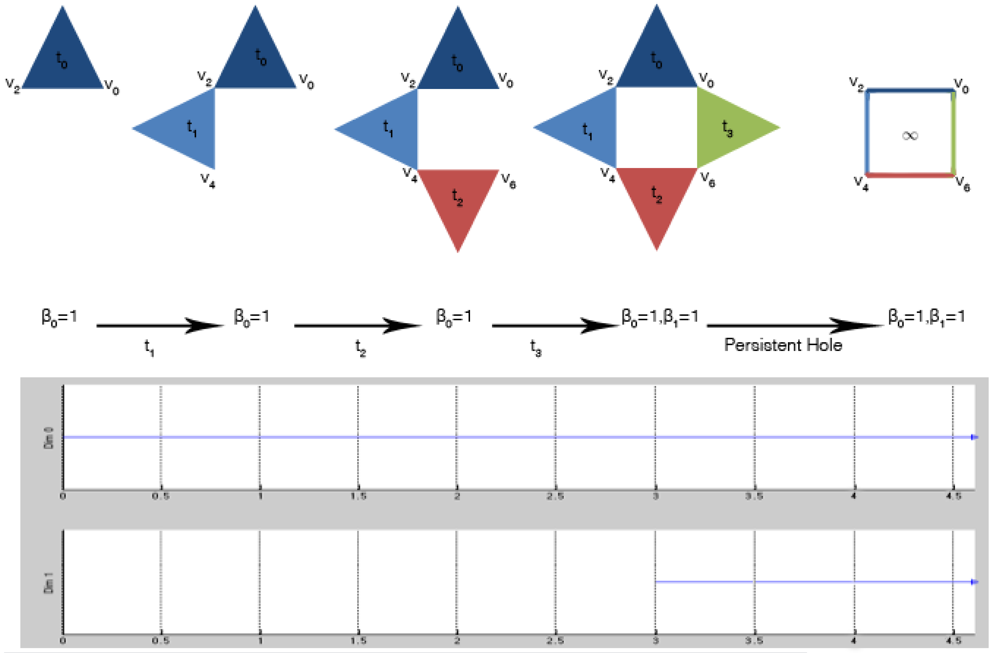
Figure 5 shows these steps applied to the filtered simplicial complex of
Figure 4. The output of the algorithm is usually graphically represented by Betti barcodes. A Betti barcode, as shown in
Figure 5, is a collection of line segments (or points in the case of persistent diagrams [
4]), where each line (labeled
Dim 0 and
Dim 1) is equipped with two pieces of information: the lifespan, in terms of appearance and disappearance, of a Betti number in the form of an interval
and the corresponding set of generators. If the line persists all over the procedure,
i.e., it survives also during the subsequent introduction of new simplices, it is called persistent, and
. Otherwise, it is classified as topological noise.
Figure 5.
Computation of persistent homology over a filtered simplicial complex: at filter value , the first 2-simplex (blue filled triangle) is introduced. The topological space is characterized by one connected component; the Betti numbers are for all . These Betti numbers are the same until when the last 2-simplex (green filled triangle) is introduced, and it is connected to the others. For filter value , the simplicial complex is still characterized by one connected component , but also by one 1-dimensional hole, i.e., . The generator of the connected component is , while the generators of the persistent hole are .
In
Figure 5, a connected component appeared at filter value
, and its set of generators is
; it is persistent, as indicated in the
Dim 0 line of the Betti barcode. Similarly, a 1-dimensional hole appeared at filter value
, and its set of generators is
; it is persistent, as indicated in the
Dim 1 line of the Betti barcode. Note that in this example, all of the lines in the barcode are persistent. However, this is not the case in general, because topological noise can be present.
At this point, we need to identify the components of the complex system interacting with each other and with the environment in which the system is immersed. Moreover, we need to characterize the latter one. Thus, from persistent homology, the methodology independently derives: (1) a set of computational agents together with their interaction matrices; and (2) the persistent entropy as a global property of the environment.
3.4. From Persistent Homology to Computational Agents: Local Interactions
Each non-empty set of generators
represents
-body interactions among components,
i.e., the methodology is able to automatically extract some hidden relationships (2-, 3-,
…,
n-relations) among system components. For instance, the persistent homology computed in
Figure 5 has non-empty sets of generators
and
.
, containing only one element, simply tells us that the data represent only one system. On the other hand,
identifies four possible 2-body interactions among four interacting components, for which the vertices
and
can be taken as representatives. In general, for each non-empty
, an interaction matrix
is obtained, such that the components (represented by vertices) can realize a multiple interaction of degree
. Note that this is a simple case of a more general model introduced by the authors in [
25], which can be associated with the data space.
Since we want to derive a computational model for the complex system under study, it is very natural to use the concept of computational agent [
2,
3] to represent the identified interacting components. An agent can execute a generic number of actions, possibly concurrently. However, TDA extracts information about connectivity among agents, but it does not provide any information regarding the agent behavior. Thus, for obtaining a complete operational model of the interactions, there is still the need to use domain-based knowledge. For instance, in
Section 4, we will use the Jerne model described in
Section 2 with higher dimensional automata [
26] as the computational model.
3.5. From Persistent Homology to Persistent Entropy: Global Information
In order to exploit global information from TDA, we use the notion of persistent entropy, introduced in [
27], to characterize the environment. This entropy measure is basically calculated using the persistent Betti barcodes. By definition, the value of the persistent entropy is strongly related to the topological structures derived from the data. Given the maximum filtration value
m of the set
F and the set
I of lines in a Betti barcode, the persistent entropy
H of the topological space is calculated as follows:
where
,
and
. Note that, when topological noise is present, for each dimension of the Betti barcode, there can be more than one line, denoted by
, with
. Instead of
, a persistent topological feature is denoted by
where
. Note that the maximum persistent entropy corresponds to the situation in which all of the lines in the barcode are of equal length. Conversely, the value of the persistent entropy decreases as more lines of different lengths are present.
Consider again the persistent homology in
Figure 5. Let the set
be such that
,
,
and
. Let
where 0 is the index of the unique line in
Dim 0 and 1 is the index of the unique line in
Dim 1 (both persistent in this case); then
; the line 0 is
; the line 1 is
; yielding an entropy
.
3.6. The Derived S[B] Model
At this point, enough information is available for defining a model of the complex system in the vision of the
paradigms, where global information constrains local interactions. Given an equilibrium condition (steady state) characterizing the system, an external or internal factor may alter this equilibrium and make the system react towards a new equilibrium [
12]. If the system is observed at a certain moment, as when a sample of the data is taken, it may still satisfy the current equilibrium condition. If not, it has entered a critical transition. Depending on the future evolution, the system can go back to the previous steady state or reach a point in which it can not go back to the previous equilibrium. Thus, it starts an adaptation phase towards a new kind of known or unknown equilibrium.
In our methodology, persistent entropy is the global information that, at the
S level, naturally constrains the local interactions at the
B level, represented by the computational model discussed in
Section 3.4. Note that we derive from the data and from the domain-specific knowledge a set of models, each of which gives an
representation of the system at the moment of the observation. The extraction of the local dynamics of the evolution of the system between two observations is beyond the scope of this work. Conversely, the global dynamics of the evolution of the system can be described in the form of a persistent entropy automaton.
3.7. Persistent Entropy Automaton
The evolution over time of the persistent entropy can be used for detecting when the system reacts to stimuli, i.e., it starts a critical transition. Let us consider the chronogram plotting the values of the persistent entropy along the observed system data samples. Indeed, a peak in the chart means an abrupt change in the topology of the simplicial complexes. This information is used to identify the time interval in which the system possibly adapts towards a new equilibrium. On the other hand, a plateau in the chart corresponds to an equilibrium condition, namely a steady state. The relevant regions can then be used for deriving a state machine representing the global observed evolution of the system.
Finite state automata [
28] are one of the most often used formalism for modeling systems (hardware, software, physical systems, and so on). They are a very familiar and useful model that extends the concept of the directed graph associating the nodes and the edges with the meaning of states and transitions, respectively. A state describes a static feature of the behavior of the system during its evolution, while a transition models how the system can evolve from one state to another. The basic formalism has been generalized in order to model timed [
29] and hybrid systems [
30]. In this paper, automata are equipped with topological information in order to model data-based complex systems.
We use the notion of persistent entropy as an observable, which is associated with the behavioral level
B, to define the equilibrium conditions characterizing the steady states of the
system. For a more formal definition of the link between the observables and the dynamics of
, we refer to [
12]. The structural level
S of the derived
model can be defined as a persistent entropy automaton (PEA), which is a tuple
where:
R is a set of steady states;
Λ is a set of names for the transitions;
is the initial steady state;
H is the observable variable, corresponding to the value of persistent entropy;
is a labeled transitions relation among steady states;
is a labeling function associating each state with its equilibrium condition, depending on the values of H.
In a PEA, the notion of time is intrinsically present, which can be continuous or discrete. The value H of the persistent entropy must be defined for each instant t in the time domain. In our methodology, the time domain is discrete, and each discrete instant t corresponds to an observation of the data, i.e., the value of the persistent entropy is the one calculated from persistent homology at each iteration and reported on the chronogram.
The dynamics of a PEA is described as follows. Whenever a PEA is in a steady state ρ, the current value of H (or a value derived from H) must satisfy the associated equilibrium condition . Time can elapse while the PEA stays in ρ, and the value of H changes accordingly. If at a certain point, the equilibrium condition is no longer satisfied, the PEA must exit the state ρ and start executing a transition . This process is in general non-instantaneous; the PEA needs some time, i.e., further changes in the value of H, in order to reach a point at which the equilibrium condition of state is satisfied. At that moment, the PEA is again in a steady state, and the dynamics is again the one previously introduced.
4. S[B] Model of the Case Study
According to Jerne [
13], the IN can be described by three main states: virgin, activation and memory. In the virgin state, there are no antibodies, but only non-specific T cells that start their activities after the activation signal sent by B cells that recognize the presence of pathogens. Then, the IN proliferates antibodies and reaches the activation state, which is not a steady state. After the activation, the IN performs the immunization, during which the antibodies play a dual role. In fact, an antibody can be seen both as a self-protein (a protein of the organism) or a non-self protein (a pathogen to be suppressed). After the immunization, the IN reaches the memory state. This state represents a steady condition in which there is only a selection of antibodies. All of the transitions and states of IN are characterized by the fact that antibodies perform basically two actions: elicitation and suppression.
In the rest of this section, we report on the application of our methodology to the IN simulated with
C-ImmSim [
16,
31]. We executed several (in the order of hundreds) simulations, each of them characterized by:
a lifespan of 2190 discrete time ticks, where a tick corresponds to three days;
a repertoire of at most antibodies, i.e., the maximum number of antibodies available during the whole simulation;
an antigen volume μL.
During the simulation, an antigen is injected, and after an unknown (simulated) transient period of time, the same antigen is injected again.
From Data to Persistent Homology
In
C-ImmSim, each idiotype (both antigens and antibodies) is represented with a bit-string, in our case of a 12-bit length. Two idiotypes
and
interact if and only if they are different, that is their Hamming distance
is such that
. The pair-wise distances among all of the idiotypes are stored in an affinity matrix. However, this does not take into account the volume of the idiotypes. For this reason, in this case study, we decided to replace it with a coexistence matrix
C where each element is a coexistent index. Given the Hamming distance
between two antibodies and their volumes
at time
t, their coexistence index is defined as follows:
where
n is the number of antibodies.
Equation (
2) expresses the fact that for lower values of affinity, the volume must be more significant, because the match between antibodies is less probable.
The coexistence matrix
C is a symmetric matrix, and each element is taken to represent a weighted arc of an undirected graph. In this way, we obtained a graph representation of our data taken from the simulation.
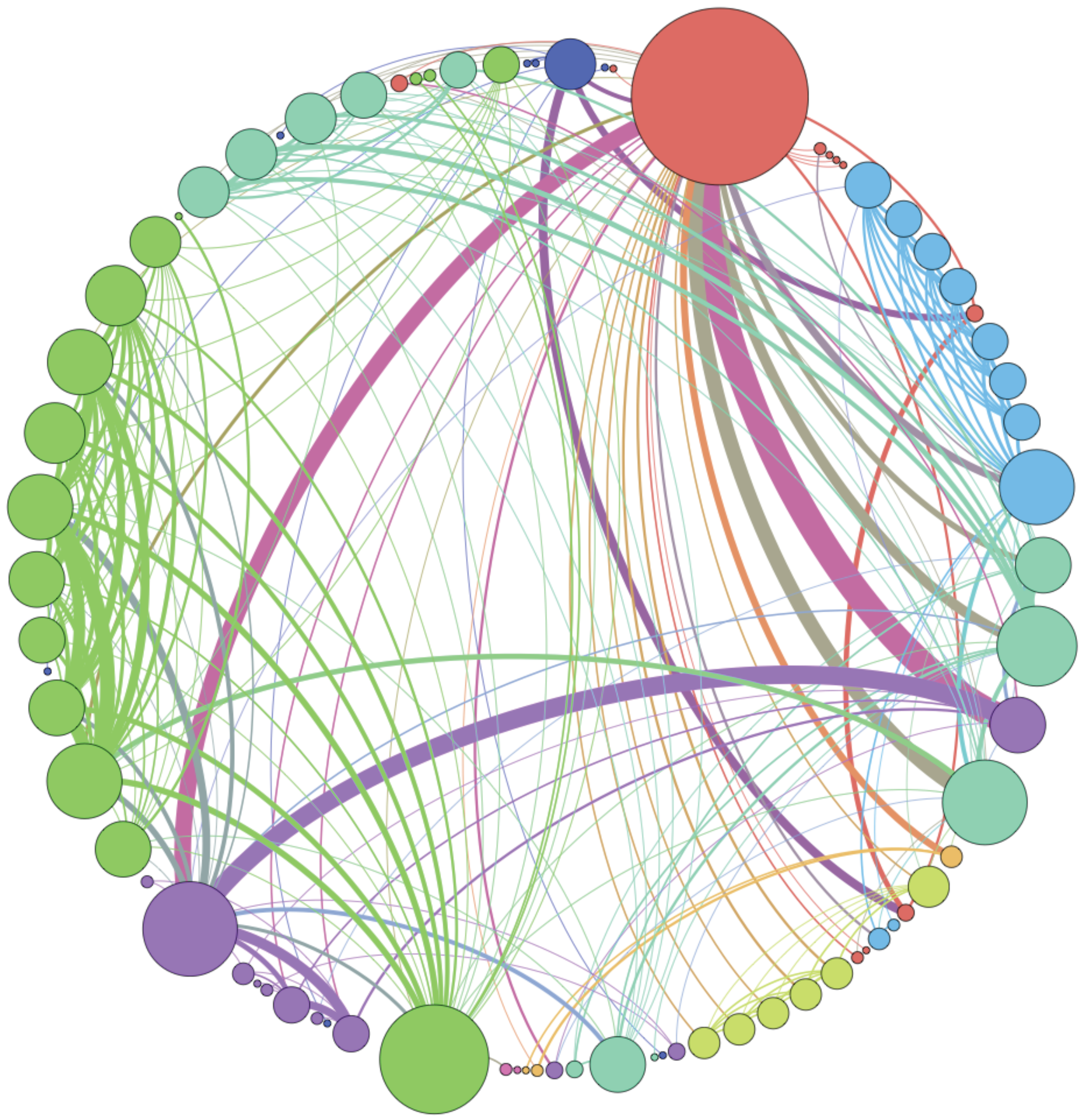
Figure 6 shows the weighted idiotypic network at the end of one simulation.
Figure 6.
Example of the immune network at the end of a simulation. The thickness of the arcs is proportional to their weight; the diameter of the nodes is proportional to the number of incident edges.
Figure 6.
Example of the immune network at the end of a simulation. The thickness of the arcs is proportional to their weight; the diameter of the nodes is proportional to the number of incident edges.
The persistent homology of the filtered simplicial complex obtained from the weighted graph was computed with jHoles [
24]. An example of the output is given in
Table 1. For each data sample, we obtained a number of one-dimensional holes in the order of hundreds. We did not obtain any persistent
n-dimensional hole with
.
Table 1.
Example of the output of jHoles with idiotypic network (IN) simulation data as the input. One connected component appeared at filtration value 0.0, which is persistent. The generator is the vertex called 16. Three 1-dimensional holes appeared at filtration values 7.0, 6.0 and 8.0, which are persistent. The four edges generating them are reported after the intervals.
| β0 | [0.0; ∞) : | {[16]} |
| β1 | [7.0; ∞) : | {[320, 3775], [256, 3775], [320, 3839], [256, 3839]} |
| [6.0; ∞) : | {[256, 3839], [256, 3711], [384, 3711], [384, 3839]} |
| [8.0; ∞) : | {[260, 3835], [260, 3839], [256, 3835], [256, 3839]} |
4.1. Idiotype Agent Behaviors as Higher Dimensional Automata
The persistent homology generated, as expected, a set of interaction matrices among entities. As introduced in
Section 3.4, we now need to select a computational model to represent the behaviors of the agents (entities), and we need to use the domain-based knowledge in order to define their actions.
Among other computational models available for expressing concurrent computations, the true concurrent characteristic of the systems considered suggests the use of higher dimensional automata for modeling the behavior of the agents.
In 1991, Pratt published the formal definition of higher dimensional automata (HDA), based on the concept of
n-dimensional objects [
26]. HDAs generalize classical automata, allowing them to express non-interleaving concurrency. States and edges of a standard finite state automaton become
n-dimensional objects where
n is any finite dimension. The basic idea is that an
n-dimensional object stands for an
n-dimensional transition representing the concurrent execution of
n actions.
Classical finite state automata are largely used for representing the behavior of concurrent and distributed systems. The components of these systems can be viewed as computational agents that execute their actions [
32].
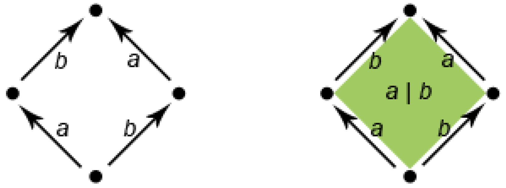
Figure 7 shows how to pass from a classical automaton to an HDA with a two-dimensional object, a surface. In the classical automaton on the left, the state at the bottom has two outgoing edges labeled
a and
b followed by
b and
a, respectively. Using an interleaving semantics, the automaton can perform both the two sequences of transitions labeled
and
. However, geometrically, the graph representing the automaton contains a hole, that is the interior of the square. Pratt suggested replacing the interleaving semantics with true concurrency by filling the hole (see
Figure 7, right). The surface, depicted on the right, represents the simultaneous execution of
a and
b without imposing any order. Conversely, the “sculpting” of the inner surface by proper transformations allows one to represent with HDAs, also classical non-determinism,
i.e., the presence of both possibilities of performing first
a and then
b or performing first
b and then
a.
Figure 7.
A classical finite state automaton representing the interleaving of actions a and b (left); the corresponding higher dimensional automaton (right).
Figure 7.
A classical finite state automaton representing the interleaving of actions a and b (left); the corresponding higher dimensional automaton (right).
Therefore,
Figure 7 shows the behavior of two different computational agents running in parallel and performing the actions
a and
b, respectively. The classical automaton on the left corresponds to the implementation of the parallelism by interleaving,
i.e., only one action can be performed at time, so the agents must execute their actions in sequence, but both sequences are possible. The HDA on the right represents a true concurrent situation in which the two agents can effectively execute their actions at the same time.
A more intuitive and concise definition of HDAs was given in terms of Chu spaces [
33,
34]. A Chu space is a tuple
over an alphabet Σ of statuses where
A is a set of actions or events,
X is a set of states and
is a function representing the status of an action or event in a state.
is an appropriate alphabet for representing actions or events that may be either unstarted or finished, as in classical automata. Conversely, an extended alphabet
is appropriate in the HDA setting, because actions or events can be unstarted, executing or finished, respectively.
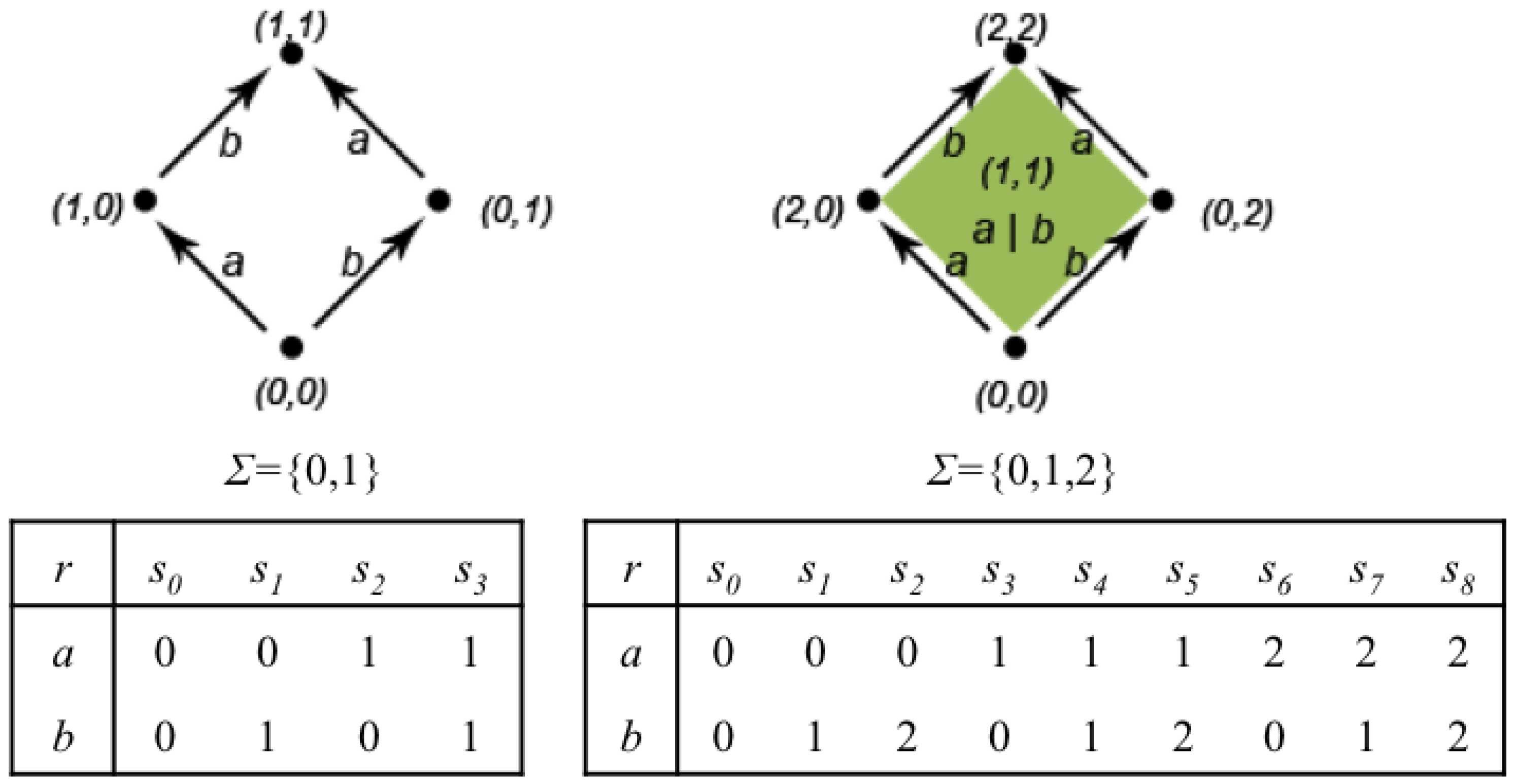
Figure 8 shows the representation as Chu spaces of the automata in
Figure 7. The function
r of the Chu spaces is represented as a matrix. Every column represents a possible state of the automaton. For instance, on the left, state
is one where both
a and
b are unstarted; state
is one in which
a is still unstarted and
b is finished, and so on. On the right, state
is the one in which action
a is unstarted and action
b is executing; state
is the one in which action
a is executing and action
b is finished, and so on.
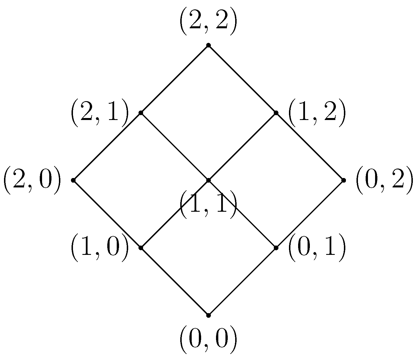
A graphical representation of a Chu space is often given using a Hasse diagram, which helps to easily deduce the set of admissible traces, dropping out automatically possibly forbidden states. In these diagrams, the computation proceeds in the upwards direction and represents an execution path in the automaton [
33]. As an example,
Figure 9 shows the Hasse diagram representing the Chu space of the HDA of
Figure 7 (right).
Figure 8.
On the left, a classical automaton together with the two-length alphabet of statuses and its Chu space representation as a matrix. On the right, a higher dimensional automaton (HDA) with its Chu space representation using the three-length alphabet.
Figure 8.
On the left, a classical automaton together with the two-length alphabet of statuses and its Chu space representation as a matrix. On the right, a higher dimensional automaton (HDA) with its Chu space representation using the three-length alphabet.
Figure 9.
Hasse diagram representing the Chu space for the concurrent execution of two actions.
Figure 9.
Hasse diagram representing the Chu space for the concurrent execution of two actions.
Applying Domain-Based Knowledge
From the Jerne model (see
Section 2), it is well known that antibodies can perform elicitation and suppression actions simultaneously on different targets. Using this domain knowledge, we modeled the antibodies given by the generators of the persistent topological features as an HDA represented by a Chu space over the three-length alphabet.
We defined an action
of the Chu space as a triple
, where
can be either elicit or reduce, and
and
are the identifiers of two antibody agents. Thus, a generic agent
can execute two possible actions concurrently, as described in the Chu space represented in
Table 2. The corresponding Hasse diagram is the one already presented in
Figure 9.
Table 2.
Chu space representation of an HDA modeling a generic antibody performing two actions on the same target .
Table 2.
Chu space representation of an HDA modeling a generic antibody performing two actions on the same target .
| r | | | | | | | | | |
|---|
| 0 | 0 | 0 | 1 | 1 | 1 | 2 | 2 | 2 |
| 0 | 1 | 2 | 0 | 1 | 2 | 0 | 1 | 2 |
Note that there is not a direct path between state to , meaning that if action is executing and action is unstarted, then the first cannot go back to the unstarted status while the second becomes executing (or vice versa). Instead, from state , it is possible to go to state , meaning that both actions can be executing at the same time. Note that if in the Hasse diagram, the line between and were not present, that would have meant that action could not start executing before action became finished. Finally, note that the actions are bi-directional, i.e., there is an elicit action from to and also an elicit action from to .
As a concrete example, we show the HDA modeling the behavior of two coupled antibodies
and
resulting from the methodology applied to the case study.
Table 3 shows the matrix of the Chu space representing such subsystem.
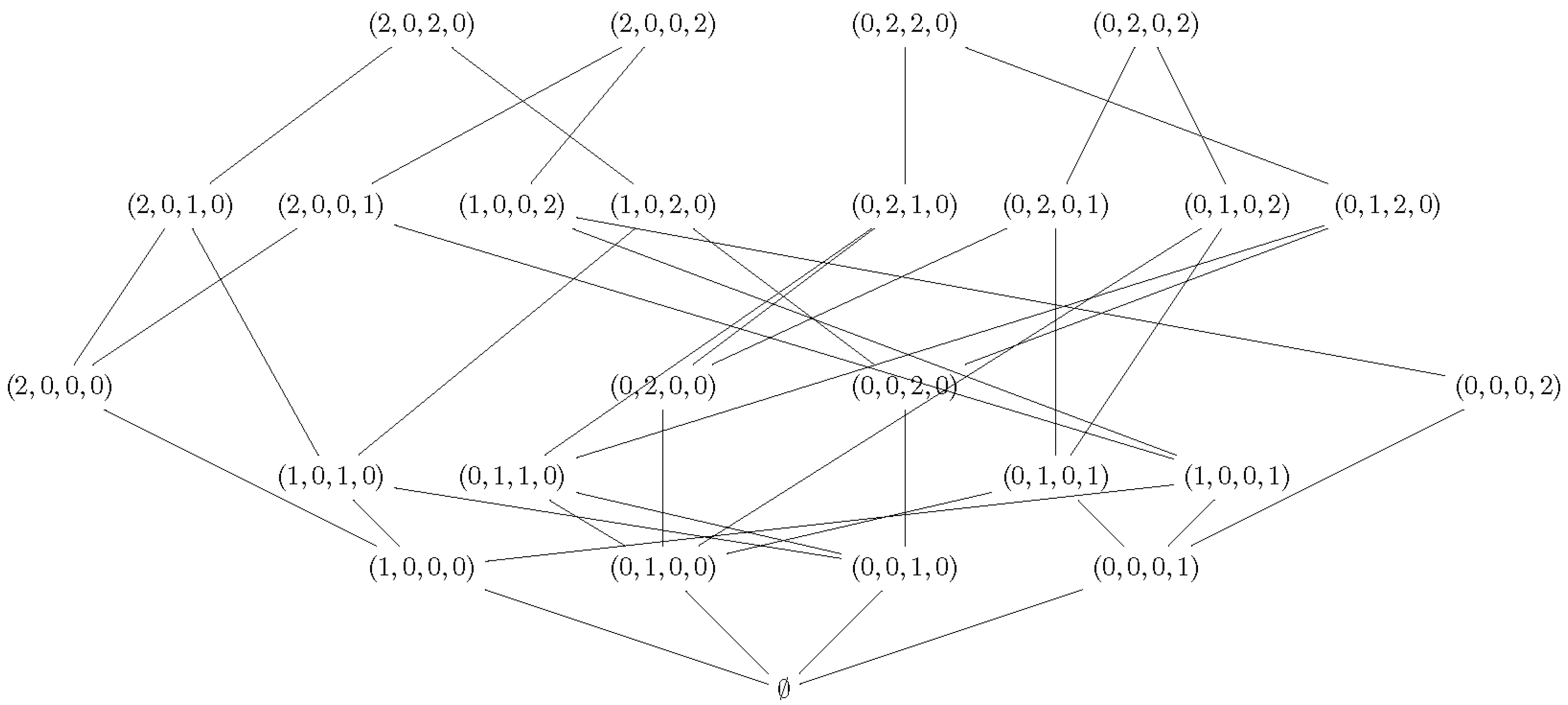
Figure 10 shows the relative Hasse diagram.
Table 3.
Chu space representing the subsystem .
Table 3.
Chu space representing the subsystem .
| r | | | | | | | | | | | | | |
|---|
| 1 | 0 | 1 | 2 | 0 | 0 | 0 | 0 | 0 | 0 | 1 | 1 | 1 |
| 0 | 0 | 0 | 0 | 1 | 2 | 0 | 0 | 0 | 0 | 0 | 0 | 0 |
| 0 | 0 | 0 | 0 | 0 | 0 | 1 | 2 | 0 | 0 | 1 | 0 | 2 |
| 2 | 0 | 0 | 0 | 0 | 0 | 0 | 0 | 1 | 2 | 0 | 1 | 0 |
| | | | | | | | | | | | | |
| 2 | 2 | 2 | 2 | 0 | 0 | 0 | 0 | 0 | 0 | 0 | 0 | |
| 0 | 0 | 0 | 0 | 1 | 1 | 1 | 1 | 2 | 2 | 2 | 2 | |
| 1 | 0 | 2 | 0 | 1 | 0 | 2 | 0 | 1 | 0 | 2 | 0 | |
| 0 | 1 | 0 | 2 | 0 | 1 | 0 | 2 | 0 | 1 | 0 | 2 | |
Figure 10.
Hasse diagram for Chu space representing the subsystem .
Figure 10.
Hasse diagram for Chu space representing the subsystem .
4.2. Persistent Entropy Automaton for the Idiotypic Network
The value
of persistent entropy associated with every observation at time
t was calculated accordingly to the definition in
Section 3.5. Note that in this case, it is possible to build a chart of
H over time, because we know that the data are subsequent, as they come from the same simulation. In general, for comparing two values of
H, one should define the so-called mass function [
35].
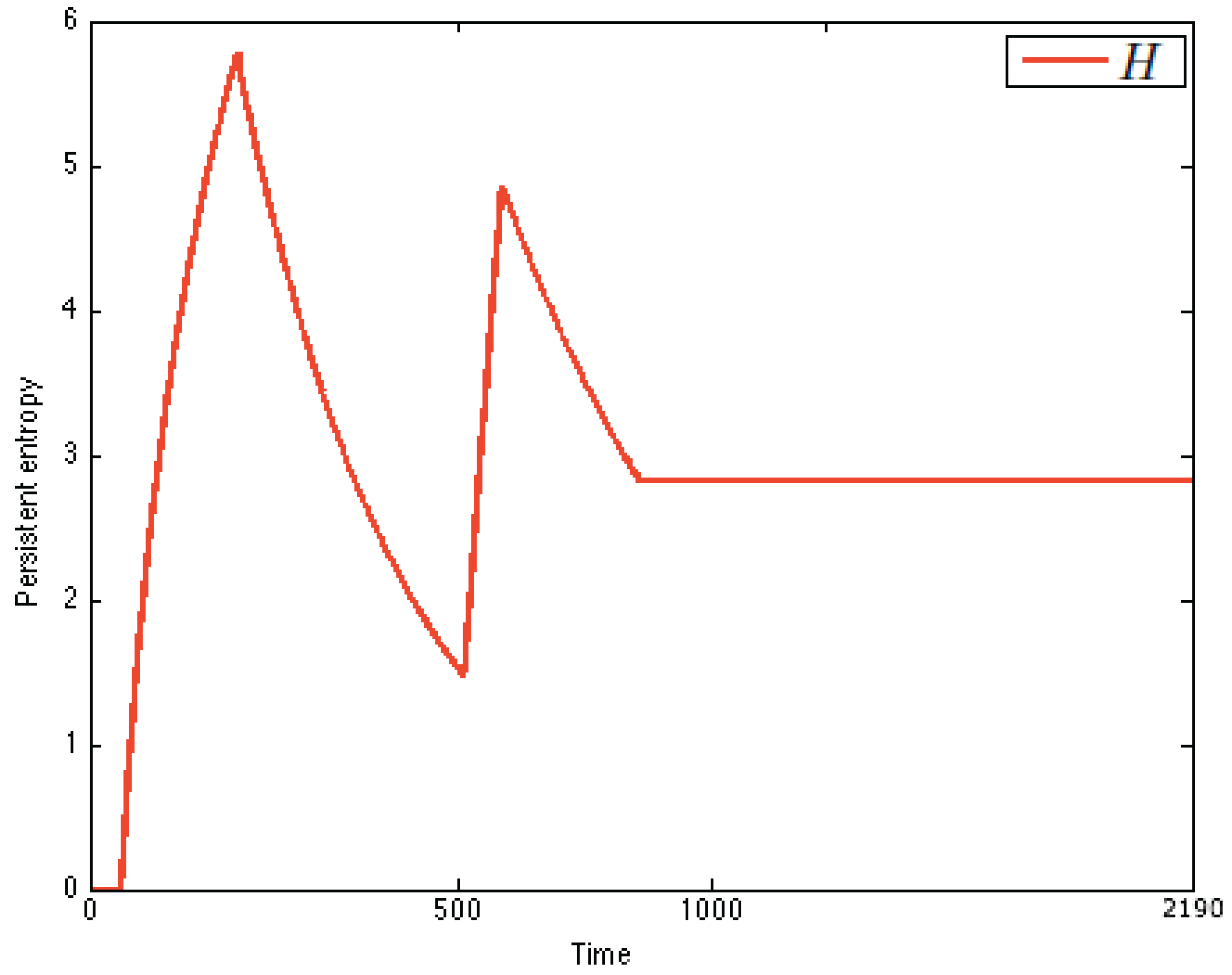
Figure 11 shows the chart of
. Persistent entropy recognizes the dynamics of the immune system: a peak in the chart means immune activation, while a plateau represents the immune memory. An upward curve between a peak and a plateau means proliferation, while a backward curve means immune response. From the comparison of the charts, it is possible to recognize that the system is stimulated twice (
Figure 11).
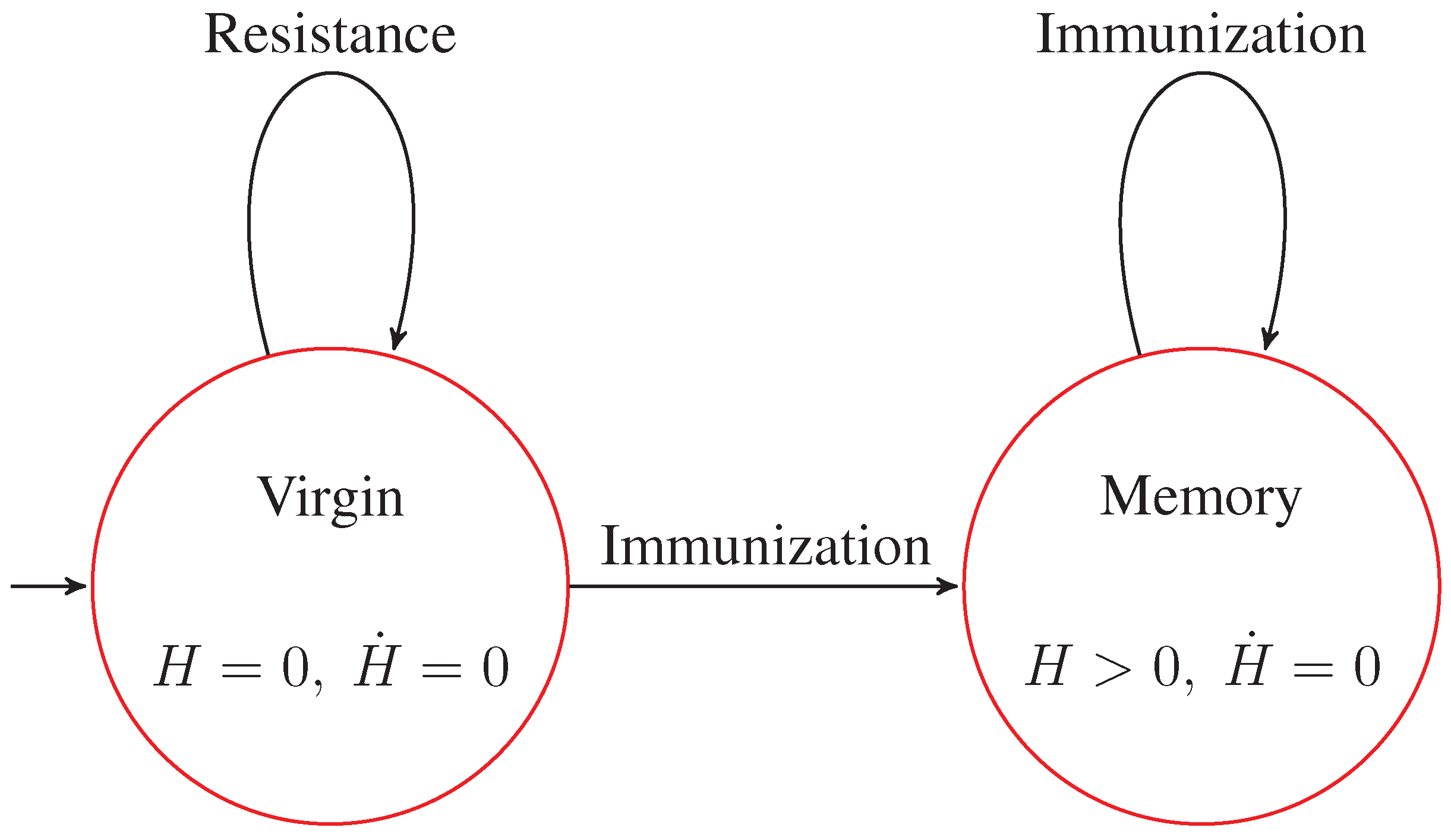
Note that from the chart, it is also possible to derive a discrete estimation of the first and second derivatives of
by using finite differences. Analyzing the chart of persistent entropy, we were able to recognize two steady states, namely virgin and memory. The virgin state of IN is characterized by the equilibrium condition
. This is the initial state in the PEA that we derived. The memory steady state corresponds to a plateau in the chart, and it is characterized by the equilibrium condition
. This information is depicted in
Figure 12 as the derived PEA.
Note that in the chart of
Figure 11, two peaks are present. This reflects the fact that the system was stimulated twice and, thus, entered a critical transition followed by an adaptation phase from state memory to itself. This then suggests that a self-transition should be added to the state memory in the PEA.
Figure 11.
Persistent entropy of the immune system. The difference between the peaks amplitude is motivated by the fact that before the second peaks, the antibodies have been already stimulated, and the immune memory has been reached, so the system is more reactive and is faster in the suppression of the antigen; thus, the the entropy value for the steady state is .
Figure 12.
Persistent entropy automaton representing the S level of the model of the idiotypic network.
Figure 12.
Persistent entropy automaton representing the S level of the model of the idiotypic network.
Finally, even if we do not observe it in our simulation, we know from domain-specific knowledge that when in the virgin state, if the received stimulus is not grater than a certain threshold, then the immune activation does not start at all, and after a while, the system goes back to the initial state again. This means that also in the initial state of the PEA, a self-loop transition should be added.


