Local Feature Extraction and Information Bottleneck-Based Segmentation of Brain Magnetic Resonance (MR) Images

Abstract

Automated tissue segmentation of brain magnetic resonance (MR) images has attracted extensive research attention. Many segmentation algorithms have been proposed for this issue. However, due to the existence of noise and intensity inhomogeneity in brain MR images, the accuracy of the segmentation results is usually unsatisfactory. In this paper, a high-accuracy brain MR image segmentation algorithm based on the information bottleneck (IB) method is presented. In this approach, the MR image is first mapped into a “local-feature space”, then the IB method segments the brain MR image through an information theoretic formulation in this local-feature space. It automatically segments the image into several clusters of voxels, by taking the intensity information and spatial information of voxels into account. Then, after the IB-based clustering, each cluster of voxels is classified into one type of brain tissue by threshold methods. The performance of the algorithm is studied based on both simulated and real T1-weighted 3D brain MR images. Our results show that, compared with other well-known brain image segmentation algorithms, the proposed algorithm can improve the accuracy of the segmentation results substantially.

1. Introduction

Based on the capability of helping brain-disease diagnosis and neuroscience research, segmentation of brain tissue in MR images is a topic of major interest in the field of brain magnetic resonance (MR). Among various segmentation schemes of brain MR images, manual segmentation performed by medical experts is usually considered to be the ground truth. However, segmenting brain MR images manually is time-consuming and highly subjective. Many automated segmentation algorithms have been proposed to solve this problem [1,2,3,4,5,6,7,8,9,10,11,12,13,14,15].

Due to the existence of various noise and artifacts in MR images [16], classical voxel-intensity-based automated segmentation methods, such as the K-means method and Gaussian mixture modeling, suffer from unsatisfactory accuracy [15,17,18]. So far, a variety of advanced methods have been proposed to improve the segmentation accuracy, for example, adding spatial constraints [1,4,8], using fuzzy methods [1,3,11,12] or using hidden Markov random field modeling [10,13]. These methods improve the segmentation accuracy to some degree, in their own way. However, to our knowledge, information theoretic methods, e.g., the information bottleneck (IB) method, have been relatively rarely studied in the field of brain MR image segmentation. Information theoretic methods have been proven very efficient in solving problems in various fields, including communication, clustering, signal processing and, even, image segmentation. Therefore, we are interested in the question of whether they can be utilized to improve the accuracy of brain MR image segmentation. We focus on the study of this question, and in this paper, we propose an IB-based segmentation algorithm, which automatically segments the brain MR images with high accuracy.

The IB method was introduced as a rigorous information theoretical framework of data quantization [19,20], offering an explicit trade-off between data fidelity and data compression in terms of information measures. Afterwards, it was widely applied to the fields of clustering [21,22,23], image segmentation [24,25], etc. Roughly speaking, the IB-based methods can be classified as “hard” and “soft”, according to the different manners of assignment/quantization (deterministic or probabilistic). In [23], the authors applied a soft-version IB method to the analysis of fMRI data, resulting in remarkable clustering results. In [24], the authors presented an image segmentation algorithm based on a hard version of the IB method and studied its performance on general images. In their segmentation approach, they first split an image with a certain strategy, then after a hard-version IB-based merging process, they obtained the final segmentation results. Due to the adoption of hard clustering, the segmentation performed by their approach has not yet revealed the full capability of the IB method on image segmentation. In this paper, we focus on the issue of segmenting brain MR images and propose a segmentation algorithm based on the soft-version IB method.

In our approach, for each voxel, we first extract a corresponding local feature, which incorporates the intensity information, not only of the voxel itself, but also of its neighbors. To some extent, the intensity information of a voxel’s neighbors implies the spatial information of the voxel. Thus, the spatial information is also incorporated into the segmentation. By accomplishing the feature extraction, all voxels in an MR image are mapped into a local-feature space. Then, a soft-version IB method performs a soft clustering in the local-feature space. By this process, one original brain MR image is clustered into several clusters of voxels. The number of final clusters is intrinsically determined by the IB method. Finally, each cluster of voxels is further classified into one kind of brain tissue by threshold methods. The proposed algorithm is studied in detail and compared with some other well-known segmentation algorithms on T1-weighted 3D brain MR images.

The paper is organized as follows. In Section 2, we present a detailed description of the proposed segmentation method. In Section 3, we validate the algorithm on both simulated and real 3D brain MR image datasets. Last, we present conclusions in Section 4.

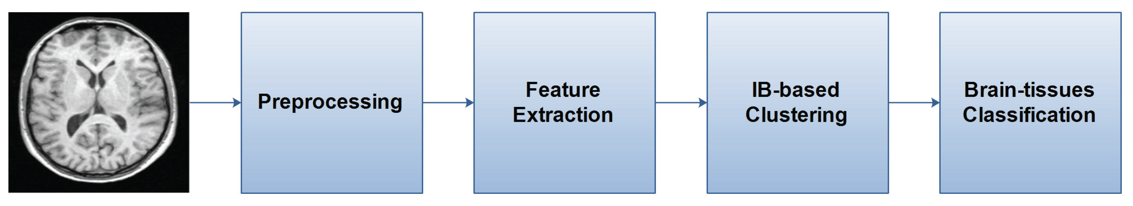
2. IB-Based Segmentation Method

In this section, we describe the IB-based segmentation method in detail. The method mainly consists of four stages, namely, a preprocessing stage, a feature extraction stage, an IB-based clustering stage and a brain-tissue classification stage. In the preprocessing stage, the brain region in the raw MR images is extracted, and the images are enhanced to increase the image contrast. This is a common stage for different segmentation methods in general, so we do not elaborate upon it here. After the preprocessing, the brain MR images are segmented further. Details of the other three stages are presented in the following subsections. Figure 1 gives the schematic description of the whole segmentation method.

Figure 1. The flow diagram of the information bottleneck (IB)-based segmentation method.

Figure 1. The flow diagram of the information bottleneck (IB)-based segmentation method.

2.1. Feature Extraction in Brain MR Images

In this stage, a local feature is extracted for each voxel in the brain MR image, which incorporates the intensity information, not only of the voxel itself, but also of its neighbors. Since there exists different kinds of noise in the brain MR images, the intensity information of an individual voxel is not enough for the high-accuracy brain-tissue classification of the voxel. Thus, we consider the intensity information of the voxel’s neighbors in addition, which reflects the local texture structure around the voxel. Hence, with the local-feature extraction, more information can be utilized in the segmentation.

In our method, the intensity of a voxel in the image is considered to be a random quantity. That is, given a brain MR image, we consider the image to be a sample of the brain imaging for a subject, with certain measurement noise. The observation equation of the brain imaging can be formulated as below:

$${\mathit{x}}_v=x_v^o+{\mathit{n}}_v$$

(1)

where ${\mathit{x}}_v$ denotes the observation intensity of the voxel, v, in the imaging samples, $x_v^o$ denotes the real intensity of the voxel, v, for the subject, and ${\mathit{n}}_v$ denotes the corresponding observation noise. The probability distribution of the observation noise is supposed to be zero-mean Gaussian with variance ${\sigma }_v^2$. Therefore, the probability distribution of the observation intensity of the voxel, v, is $p\left({\mathit{x}}_v\right)=p\left(\mathit{x}\right|v)=\mathcal{N}(x_v^o,{\sigma }_v)$. The parameters of the normal distribution can be estimated from multiple images of the same subject. When there is only one image for a subject, the value of $x_v^o$ can be simply estimated as the current observation intensity of the voxel, v, in the sole image, and the value of ${\sigma }_v$ can be determined by reasonable assumptions.

As the intensity of a voxel is a random variable, the local feature corresponding to the voxel is also considered to be a random quantity. Here, we do not give the explicit expression for the local feature, but describe the feature through its probability distribution. For the voxel, v, we construct the distribution of its corresponding local feature, ${\gamma }_v$, based on the intensity distributions of the voxel, v, itself and of its $l^2-1$ neighbors within a window of size $l\times l$, as below (We use a 2D window rather than a 3D window, because the method proposed is performed on 3D volumes slice by slice in this paper. Moreover, in many cases, the resolution of the voxel might not be the same for different dimensions, e.g.,1 mm * 1 mm * 5 mm. In such cases, the neighbors along the thick dimension actually are not the same “near” as those along thin dimensions in the sense of anatomy.):

$$\left\{\begin{array}{c}q\left({\gamma }_v\right)=p\left({\mathit{x}}_v\right)+\frac{1}{l^2-1}[p\left({\mathit{x}}_{v,1}\right)+\cdots +p\left({\mathit{x}}_{v,l^2-1}\right)]\hfill \\ p\left(\gamma \right|v)=p\left({\gamma }_v\right)=\frac{q\left({\gamma }_v\right)}{{\sum }_{{\gamma }_v}q\left({\gamma }_v\right)}\hfill \end{array}\right.$$

(2)

where the notation, $p\left({\mathit{x}}_{v,j}\right)$, means the intensity distribution of the jth neighboring voxel of voxel v. Note that the equal signs here represent the equal relationship between two functions rather than two values. More specifically, if we take the first equation above, for example, the equal sign means that, for an arbitrary value, r, in the support of the function, $q\left({\gamma }_v\right)$ (which is the union of the supports of the $l^2$ probability distributions in the right-hand side of the equation), we have:

$$q({\gamma }_v=r)=p({\mathit{x}}_v=r)+\frac{1}{l^2-1}[p({\mathit{x}}_{v,1}=r)+\cdots +p({\mathit{x}}_{v,l^2-1}=r)]$$

The distribution of the voxel feature, ${\gamma }_v$, and the distribution of the voxel intensity, ${\mathit{x}}_v$, may have supports in the same range, but in essence, voxel feature and voxel intensity are two random quantities of different meanings. The first Equation in (2) combines the the intensity distributions of the central voxel, v, and of the surrounding $l^2-1$ neighboring voxels within the window, resulting in a combination distribution, $q\left({\gamma }_v\right)$. The two terms in the right-hand side of the first equation reflect the intensity information of the central voxel and the neighboring voxels, respectively, while the coefficient, $\frac{1}{l^2-1}$, balances these two kinds of information. Here, the weighting coefficient can be further made adjustable by adding a free parameter, α, resulting in $\frac{\alpha }{l^2-1}$. In this paper, we let the weighting coefficient be a constant ($\frac{1}{l^2-1}$), for the reasons that this setting can lead to satisfactory segmentation results, as well as reduce the number of free parameters. The second Equation in (2) normalizes the combination distribution, to make the distribution a real probability distribution. We view the normalized combination distribution as the probability distribution of a new random quantity, which is exactly the local feature corresponding to the voxel, v. By this way, we get the statistical information of the local feature for a voxel.

For a brain MR image consisting of N voxel, denoted as an integer set $V=\{1,2,\cdots ,N\}$, we get N corresponding probability distributions of voxel feature, $\left\{p\right(\gamma \left|v\right);v\in V\}$. Besides, the probability distribution of a feature over the whole image can be calculated as $p\left(\gamma \right)={\sum }_{v}p\left(\gamma \right|v)$, which describes the global information contained in the image. Thus, we have mapped the original brain MR image into a feature space of interest, Γ, and have gotten the relevant feature information over the whole image. In the following stage, the soft-version IB method clusters voxels of the image in such a feature space.

2.2. IB-Based Clustering

The IB method was first proposed as a rigorous information theoretical framework of data quantization [19,20], offering an explicit tradeoff between data fidelity and data compression in the sense of information measures. For input data, the IB method outputs a compressed representation, which has the largest mutual information with the input data, at a given degree of data compression. In the case of image segmentation, we want to segment the image consisting of N voxels into a few numbers of clusters of voxels, for example, M clusters, with $M<N$. Therefore, the segmentation results can be naturally viewed as a kind of compressed representation of the original image. In the following, we first describe the problem of MR image segmentation from the perspective of data compression mathematically, then we give the solution to the problem based on the IB method.

Given a brain image consisting of N voxels, denoted as an integer set $V=\{1,2,\cdots ,N\}$, and given a feature space of interest, Γ, for segmentation, we need to assign a cluster label, $k\in K=\{1,2,\cdots ,M\}$, for each voxel, $v\in V$, according to their corresponding features. In a soft clustering, the assignment is described by the conditional probabilities, $p\left(k\right|v),k\in K,v\in V$. Here, the voxel label and cluster label are viewed as two random quantities, v and k, respectively, with their value, $v\in V,k\in K$. The clustering re-quantifies the image information, which is described in the feature space, Γ, from N levels/voxels to M levels/clusters. To obtain good segmentation results, we need to make the clustering results retain as much image information as possible, while compressing the image data to a certain degree. This object leads to the minimization of the cost function of the IB method:

$$\mathcal{L}\left[p\right(k\left|v\right)]=I(\mathit{v};\mathit{k})-\beta \mathit{I}(\mathit{k};\gamma )$$

(3)

where $I(\mathit{v};\mathit{k})$ is the mutual information between the original presentation, v, and the compressed representation/re-quantification, k, $I(\mathit{k};\gamma )$ is the mutual information between the compressed representation, k, and the feature of image γ in the space, Γ, and β is a positive-weighting coefficient. A high degree of data compression usually indicates a small $I(\mathit{v};\mathit{k})$, while a high degree of data fidelity means a large $I(\mathit{k};\gamma )$. Thus, this cost function gives an explicit tradeoff between the image data compression and the image data fidelity, in the sense of mutual information. For the minimization of the functional (3), in [19], the authors provided an iterative solution, as below (τ is the iteration step):

$$\left\{\begin{array}{c}{p}_{\tau }\left(k\right|v)=\frac{p_{\tau }\left(k\right)}{Z_{\tau }(v,\beta )}exp(-\beta d_{\tau }(v,k))\hfill \\ p_{\tau +1}\left(k\right)=\sum _{v}p\left(v\right)p_{\tau }\left(k\right|v)\hfill \\ p_{\tau +1}\left(\gamma \right|k)=\sum _{\gamma }p\left(\gamma \right|v)p_{\tau }\left(v\right|k)\hfill \end{array}\right.$$

(4)

where:

$$d_{\tau }(v,k)=\sum _{\gamma }p\left(\gamma \right|v)log\frac{p\left(\gamma \right|v)}{p_{\tau }\left(\gamma \right|k)}$$

(5)

is the Kullback-Leibler divergence [26] between $p\left(\gamma \right|v)$ and $p_{\tau }\left(\gamma \right|k)$ and:

$$Z_{\tau }(v,\beta )=\sum _k{p}_{\tau }\left(k\right)exp\left(\beta d_{\tau }(v,k)\right)$$

(6)

Before performing the iterative algorithm above, we need to determine several initial conditions, including the number of clusters, $M_{\text{initial}}$, the probabilities, $p_0\left(k\right|v)$ and $p\left(v\right)$, etc. The initialization steps for image segmentation are as below: (a) initialize $p\left(v\right)=1/N,v\in V$, which means a uniform prior distribution of the voxels; (b) perform the voxel-intensity-based K-means clustering method (with $M_{\text{initial}}$ preset) on the image first, then initialize the “soft assignment”, $p_0\left(k\right|v)$, according to the result of the k-means clustering, that is, for voxel v, $p_0\left(k\right|v),k\in K$ is set at large probabilities at the cluster label given by the k-means clustering and is set at small probabilities at other cluster labels; (c) initialize $p_0\left(k\right)$, $p_0\left(v\right|k)$ and $p_0\left(\gamma \right|k)$ according to the complete probability formula and the Bayes rule, as below:

$$\left\{\begin{array}{c}{p}_0\left(k\right)=\sum _{v}p\left(v\right)p_0\left(k\right|v)\hfill \\ p_0\left(v\right|k)=\frac{p\left(v\right)p_0\left(k\right|v)}{p_0\left(k\right)}\hfill \\ p_0\left(\gamma \right|k)=\sum _v{p}_0\left(\gamma \right|v)p_0\left(v\right|k)\hfill \end{array}\right.$$

(7)

After accomplishing the initialization steps, we perform the iteration process (4) until the algorithm converges, then we get the final probabilistic assignment, $p_{\text{final}}\left(k\right|v)$. At last, for each voxel v, we let the cluster label, $k_0$, which corresponds to the largest probability, $p_{\text{final}}\left(k_0\right|v)$, be its final cluster label. Note that, after performing such a decision, the probabilities of some clusters, $p\left(k\right)$, may reach zero, leading to a smaller number of final clusters, $M_{\text{final}}$, $M_{\text{final}}<M_{\text{initial}}$.

In the soft IB method, the number of final clusters, $M_{\text{final}}$, is affected by the value of β, which controls the tradeoff between data fidelity and data compression. A large value of β increases the weight of data fidelity, resulting in an $M_{\text{final}}$ close to the initial set, $M_{\text{initial}}$, while a small value of β increases the weight of data compression, resulting in an $M_{\text{final}}$ close to one. In general, $\beta \ge 1$ is necessary for the soft IB method to converge toward an optimal solution [27]. Besides, the number of final clusters, $M_{\text{final}}$, is also naturally affected by the input image. Qualitatively, under a fixed β, a complicated image results in an $M_{\text{final}}$ close to the initial set, $M_{\text{initial}}$, while a simple image results in a smaller $M_{\text{final}}$.

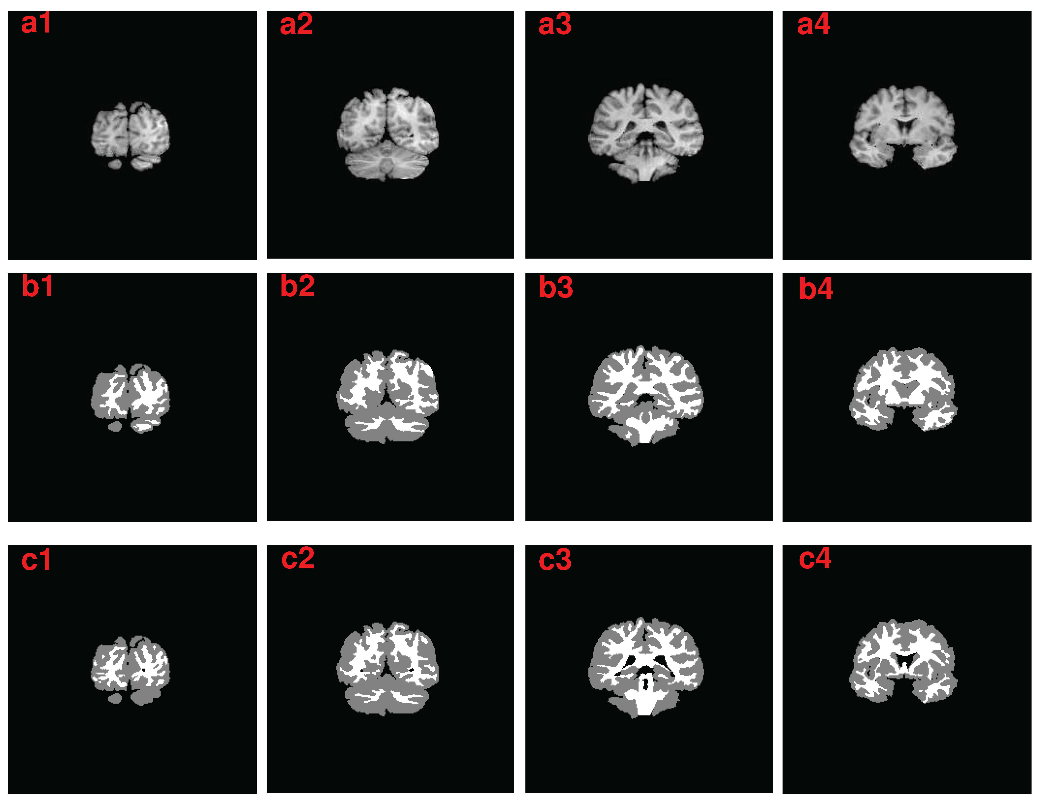
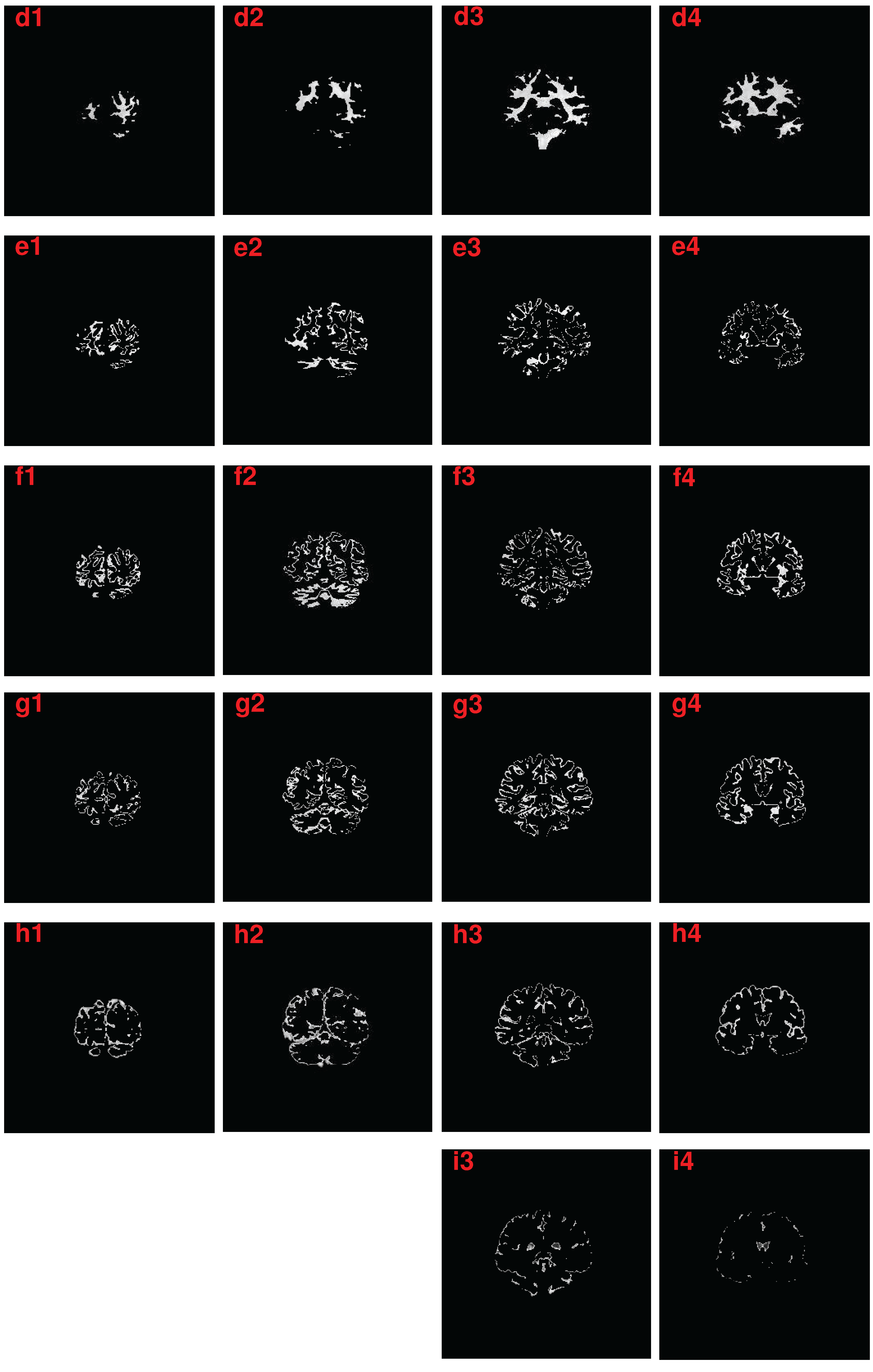
2.3. Brain Tissue Classification

After the feature extraction and IB-based clustering, the brain MR image is automatically segmented into several clusters of voxels, with the number of clusters affected jointly by the value of β and the input image. To segment the image into several brain tissues of interest, in this stage, we further classify each of the clusters into a certain type of brain tissue. Here, we focus on two main brain tissues, white matter (WM) and gray matter (GM).

We accomplish the classification by simple threshold methods. First, we calculate a global intensity threshold of the whole image using classical threshold methods, such as the mean method or the OTSUmethod [28,29]. Second, we compare the mean intensity of each cluster with the global intensity threshold. The cluster of voxels with mean intensity larger than the global intensity threshold is classified as white matter, and vice verse. Note that, classification of an individual voxel according to its intensity is usually not accurate in a noisy case. In contrast, with noisy voxels having been clustered into several clusters based on the information of local features, classification of these voxel-clusters according to their mean intensity is more robust. Therefore, in this stage, we adopt such a simple classification procedure. The accuracy of segmentation with this kind of classification will be tested in the next section.

3. Results and Discussion

In this section, we evaluate the proposed segmentation method through a set of experiments. The experiments are based on a simulated brain MR image set and a real brain MR image set. The simulated dataset is taken from the BrainWeb repository [30]. It consists of simulated 3D T1-weighted MR images (eight bits) with various levels of noise and spatial inhomogeneity. The real dataset is taken from the Internet brain segmentation repository (IBSR) [31]. It consists of 20 real normal 3D T1-weighted brain MR images (eight bits). In the real image set, each brain MR image has a corresponding ground-truth segmentation result generated by trained investigators using semiautomated segmentation algorithms [32]. These two image data sets have been widely used in the evaluation of brain MR image segmentation algorithms [1,2,8].

In the proposed method, there are two main free parameters, the weighting coefficient, β, and the initial cluster number, $M_{\text{initial}}$. In the following experiments, we first evaluate the performance of the algorithm on both simulated and real image sets based on empirically selected parameters, then we study the joint effect of the two parameters based on two representative real brain images. We evaluate the segmentation results by comparing them with the corresponding ground truths, and we adopt the Tanimoto coefficient [31] as the overlap metric in comparison, which is also adopted by the IBSR. Besides, the algorithm is performed on the 3D images slice by slice.

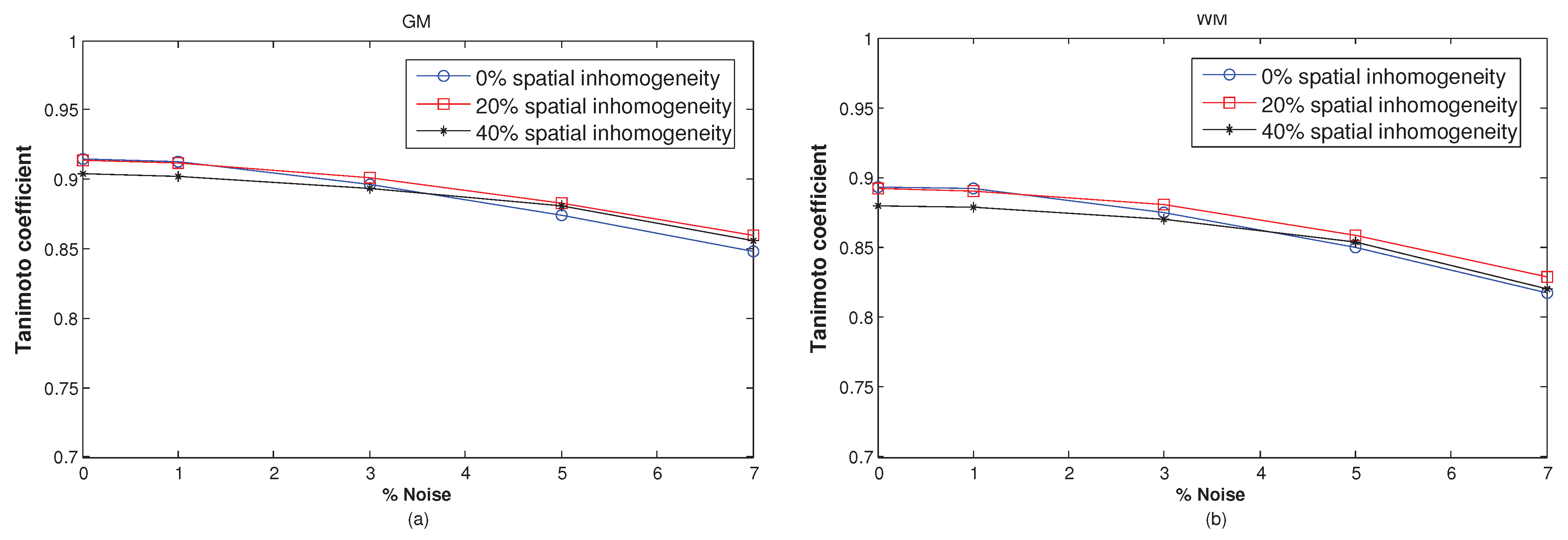
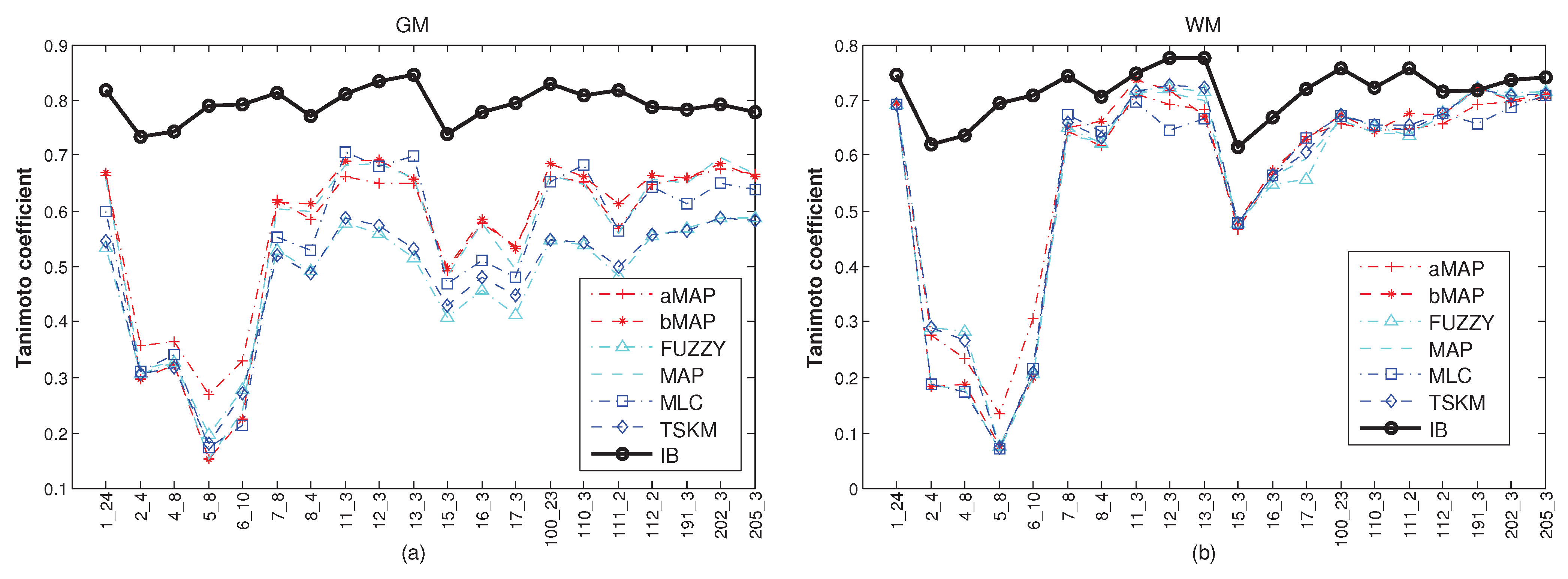
3.1. Performance of the Algorithm under Empirical Parameters

In this part, we set $\beta =1.6$, $M_{\text{initial}}=6$. Since for each subject, there is only one volume in the image set, we assume the standard deviation of noise to be seven, which is about 3% of the maximal intensity level of an eight-bit image. Other reasonable values, such as five or 10, do not affect the final results much for the segmentation of brain MR images. Besides, the window size used in the feature extraction is $3\times 3$.

Firstly, we evaluate the proposed method on the simulated image set. Figure 2 shows the performance of the method under five different noise levels and three different inhomogeneity levels. From the results, we see that the proposed method can obtain high-accuracy segmentation results (with Tanimoto coefficients nearing one) for the simulated data, and it is robust to the noise and inhomogeneity. We explain the reasons for the robustness of the method as follows. Since the 3D images are processed slice by slice, the intensity threshold for brain tissue classification is calculated within each slice, and its value is, thus, different for different slices. This makes the algorithm robust to inter-slice intensity inhomogeneity. Besides, the enhancement of the slice image in the preprocessing stage and the adoption of local feature and information measures help the method to be robust to noise and intra-slice bias.

Figure 2. Tanimoto’s performance metric of the proposed segmentation algorithm on the simulated 3D brain magnetic resonance (MR) images from BrainWeb. (a) For gray matter (GM) segmentation; (b) for white matter (WM) segmentation.

Figure 2. Tanimoto’s performance metric of the proposed segmentation algorithm on the simulated 3D brain magnetic resonance (MR) images from BrainWeb. (a) For gray matter (GM) segmentation; (b) for white matter (WM) segmentation.

Secondly, we evaluate the proposed method on the real image set. The IBSR provides the performance of six well-known segmentation algorithms on the same image set for convenient comparison, including the maximum a posteriori probability (MAP), adaptive MAP (aMAP), biased MAP (bMAP), fuzzy c-means (FUZZY), tree-structure k-means (TSKM) and Maximum Likelihood (MLC). In Figure 3, we show the segmentation accuracy of our algorithm and of the above six algorithms. We see that our algorithm has a significant performance advantage to the six algorithms and obtains high-accuracy segmentation results for real images with different levels of noise. In Figure 4, we show four real example images of the MR scans, their corresponding segmentation results produced by our algorithm and the corresponding ground truths. The segmentation results show high similarity with the corresponding ground truths. In Figure 5, we further show the detailed IB-based clustering results for the same four real examples of MR scans. From these results, we see that the IB method clusters each MR slice image into five or six clusters of voxels at the current setting of parameters. The voxel-clusters, d1–d4 and e1–e4, with mean intensities above the threshold, are finally classified as white matter, while other voxel-clusters are finally classified as gray matter. Note that, for real MR images, a3 and a4, the IB method actually obtains the voxel-clusters corresponding to cerebrospinal fluid (see i3 and i4), which have very low intensity in the original MR images. In this paper, we only focus on the classification of gray matter and white matter. Therefore, these voxel-clusters, with mean intensities far below the threshold, are finally classified as gray matter.

Figure 3. Tanimoto’s performance metric of different segmentation algorithms on 20 normal 3D brain MR images from the Internet brain segmentation repository (IBSR). (a) For GM segmentation; (b) for WM segmentation.

Figure 3. Tanimoto’s performance metric of different segmentation algorithms on 20 normal 3D brain MR images from the Internet brain segmentation repository (IBSR). (a) For GM segmentation; (b) for WM segmentation.

Figure 4. Four real T1-weighted brain MR images (first row), the corresponding segmentation results obtained by our algorithms (second row) and the corresponding ground truths (third row).

Figure 4. Four real T1-weighted brain MR images (first row), the corresponding segmentation results obtained by our algorithms (second row) and the corresponding ground truths (third row).

Figure 5. Detailed IB-based clustering results for the same four examples of MR scans as those shown in Figure 4 (a1–a4). Results displayed in one column correspond to one example.

Figure 5. Detailed IB-based clustering results for the same four examples of MR scans as those shown in Figure 4 (a1–a4). Results displayed in one column correspond to one example.

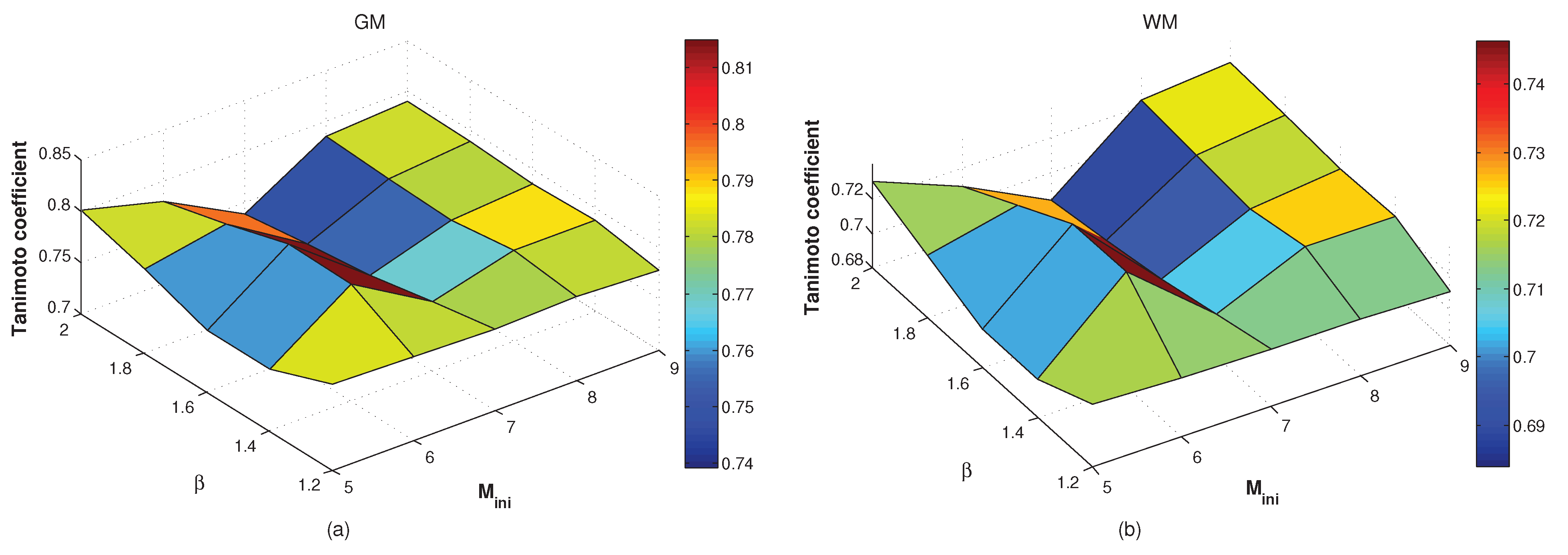
3.2. Effect of the Free Parameters on the Algorithm’s Performance

In this part, we choose two representative real brain images, $“1\_24”$ and $“15\_3”$, which are of high segmentation accuracy (with low level noise) and of relatively low segmentation accuracy (with high level noise), respectively, to study the joint effect of the free parameters on the performance of the proposed algorithm.

Figure 6. Tanimoto’s performance metric of our algorithm under different values of β and $M_{\text{initial}}$ for the image, $“1\_24”$. (a) For GM segmentation; (b) for WM segmentation.

Figure 6. Tanimoto’s performance metric of our algorithm under different values of β and $M_{\text{initial}}$ for the image, $“1\_24”$. (a) For GM segmentation; (b) for WM segmentation.

Figure 7. Tanimoto’s performance metric of our algorithm under different value of β and $M_{\text{initial}}$ for the image, $“15\_3”$. (a) For GM segmentation; (b) for WM segmentation.

Figure 7. Tanimoto’s performance metric of our algorithm under different value of β and $M_{\text{initial}}$ for the image, $“15\_3”$. (a) For GM segmentation; (b) for WM segmentation.

Here, we let the value of $M_{\text{initial}}$ vary in [5,9] and let the value of β vary in [1.2, 2.0]. Values of other parameters are set the same as those adopted in the above experiments. When $\beta <1.2$, the cost function of IB gives an insufficient weighting for the data fidelity, making the number of final clusters be one. When $\beta >2.0$, the cost function of IB gives a large weighting for the data fidelity, making the number of final cluster $M_{\text{final}}=M_{\text{initial}}$. Figure 6 shows the segmentation accuracy of our algorithm under different values of β and $M_{\text{initial}}$ for the image, $“1\_24”$, while Figure 7 shows the same kind of performance evaluation for the image, $“15\_3”$. From these surface plots, we see that, under a wide range of parameter values, our algorithm can obtain high-accuracy segmentation results for real images with different levels of noise. These results show that our algorithm has a certain degree of tolerance for parameter-value selection.

4. Conclusions

In this paper, we have proposed a new approach for brain MR image segmentation. This approach first maps the original image to a local-feature space, which incorporates the intensity information of both the central voxel and the neighboring voxels. Then, the soft-version IB method clusters the voxels in the feature space. Finally, the clusters of voxels are classified into brain tissues by threshold methods. We have validated the performance of the proposed algorithm on both simulated and real T1-weighted brain image sets in detail. Our results show that, compared with some other well-known brain image segmentation algorithms, the proposed algorithm can improve the segmentation accuracy substantially.

References

1. Ji, Z.X.; Xia, Y.; Sun, Q.S.; Chen, Q.; Xia, D.S.; Feng, D.D. Fuzzy local gaussian mixture model for brain MR image segmentation. IEEE Trans. Inf. Technol. Biomed. 2012, 16, 339–337. [Google Scholar] [PubMed]
2. Tian, G.J.; Xia, Y.; Zhang, Y. Hybrid genetic and variational expectation-maximization algorithm for GMM based brain MR image segmentation. IEEE Trans. Inf. Technol. Biomed. 2011, 15, 373–380. [Google Scholar] [CrossRef] [PubMed]
3. Ji, Z.X.; Sun, Q.S.; Xia, D.S. A modified possibilistic fuzzy C-means clustering algorithm for bias field estimation and segmentation of brain MR image. Comput. Med. Imag. Graph. 2011, 35, 383–397. [Google Scholar] [CrossRef] [PubMed]
4. Liao, L.; Lin, T.; Li, B. MRI brain image segmentation and bias field correction based on fast spatially constrained kernel clustering approach. Pattern Recog. Lett. 2008, 29, 1580–1588. [Google Scholar] [CrossRef]
5. Sfikas, G.; Nikou, C.; Galatsanos, N.; Heinrich, C. MR brain tissue classification using an edge-preserving spatially variant bayesian mixture model. Med. Image. Comput. Comput. Assist. 2008, 11, 43–50. [Google Scholar]
6. Song, T.; Jamshidi, M.M.; Lee, R.R.; Huang, M. A modified probabilistic neural network for partial volume segmentation in brain MR image. IEEE Trans. Neural Netw. 2007, 18, 1424–1432. [Google Scholar] [CrossRef] [PubMed]
7. Chang, H.; Valentino, D.J.; Duckwiler, G.R.; Toga, A.W. Segmentation of brain MR images using a charged fluid model. IEEE Trans. Biomed. Eng. 2007, 54, 1798–1813. [Google Scholar] [CrossRef] [PubMed]
8. Greenspan, H.; Ruf, A.; Goldberger, J. Constrained gaussian mixture model framework for automatic segmentation of MR brain images. IEEE Trans. Med. Imag. 2006, 25, 1233–1245. [Google Scholar] [CrossRef]
9. Li, X.; Li, L.; Lu, H.; Liang, Z. Partial volume segmentation of brain magnetic resonance images based on maximum a posteriori probability. Med. Phys. 2005, 32, 2337–2345. [Google Scholar] [CrossRef] [PubMed]
10. Chen, T.; Huang, T.S.; Liang, Z.P. Segmentation of Brain MR Images Using Hidden Markov Random Field Model with Weighting Neighborhood System. In Proceedings of the IEEE 2004 Nuclear Science Symposium Conference Record, Rome, Italy, 16–22 October 2004; Volume 5, pp. 3209–3212.
11. Liew, A.; Yan, H. An adaptive spatial fuzzy clustering algorithm for 3-D MR image segmentation. IEEE Trans. Med. Imag. 2003, 22, 1063–1075. [Google Scholar] [CrossRef] [PubMed]
12. Ahmed, M.; Yamany, S.; Mohamed, N.; Farag, A.; Moriarty, T. A modified fuzzy C-means algorithm for bias field estimation and segmentation of MRI data. IEEE Trans. Med. Imag. 2002, 21, 193–199. [Google Scholar] [CrossRef] [PubMed]
13. Zhang, Y.; Brady, M.; Smith, S. Segmentation of brain MR images through a hidden markov random field model and the expectation maximization algorithm. IEEE Trans. Med. Imag. 2001, 20, 45–57. [Google Scholar] [CrossRef] [PubMed]
14. Pham, D.L.; Xu, C.; Prince, J.L. Current methods in medical image segmentation. Ann. Rev. Biomed. Eng. 2000, 2, 315–337. [Google Scholar] [CrossRef] [PubMed]
15. Wells, W.; Grimson, E.; Kikinis, R.; Jolesz, F. Adaptive segmentation of MRI data. IEEE Trans. Med. Imag. 1996, 15, 429–442. [Google Scholar] [CrossRef] [PubMed]
16. Macovski, A. Noise in MRI. Magn. Reson. Med. 1996, 36, 494–497. [Google Scholar] [CrossRef] [PubMed]
17. Kapur, T.; Grimson, W.E.; Wells, W.M.; Kikinis, R. Segmentation of brain tissue from magnetic resonance images. Med. Image Anal. 1996, 1, 109–127. [Google Scholar] [CrossRef]
18. Gupta, L.; Sortrakul, T. A gaussian-mixture-based image segmentation algorithm. Pattern Recog. 1998, 31, 315–325. [Google Scholar] [CrossRef]
19. Tishby, N.; Pereira, F.; Bialek, W. The Information Bottleneck Method. In Proceedings of the 37th Annual Allerton Conference Communicaiton, Control and Computing, Monticello, IL, USA, September 1999; pp. 368–377.
20. Slonim, N.; Tishby, N. Agglomerative information bottleneck. Adv. Neural Inf. Process. Syst. 1999, 12, 617–623. [Google Scholar]
21. Gordon, S.; Greenspan, H.; Goldberger, J. Applying the Information Bottleneck Principle to Unsupervised Clustering of Discrete and Continuous Image Representations. In Proceedings of the Ninth IEEE 2003 International Conference Computer Vision, Nice, France, 13–16 October 2003; Volume 1, pp. 370–377.
22. Slonim, N.; Tishby, N. Document Clustering Using Word Clusters via The Information Bottleneck Method. In Proceedings of the 23rd Annual International ACM SIGIR Conference on Research and Development in Information Retrieval, Athens, Greece, 24–28 July 2000; pp. 208–215.
23. Thirion, B.; Faugeras, O. Feature characterization in fMRI data: The information bottleneck approach. Med. Image Anal. 2003, 8, 403–419. [Google Scholar] [CrossRef] [PubMed]
24. Bardera, A.; Rigau, J.; Boada, I.; Feixas, M.; Sbert, M. Image segmentation using information bottleneck method. IEEE Trans. Image Process. 2009, 18, 1601–1612. [Google Scholar] [CrossRef] [PubMed]
25. Bardera, A.; Feixas, M.; Boada, I. Registration-Based Segmentation Using the Information Bottleneck Method. In Proceedings of the Iberian Conference on Patern Recognition and Image Analisys, Girona, Spain, 6–8 June 2007; Volume 2. pp. 190–197.
26. Cover, T.M.; Thomas, J.A. Elements of Information Theory, 2nd ed.; John Wiley and Sons: Hoboken, NJ, USA, 2006. [Google Scholar]
27. Still, S.; Bialek, W.; Bottou, L. Geometric clustering using the information bottleneck method. Adv. Neural Inf. Process. Syst. 2003, 16, 1165–1172. [Google Scholar]
28. Sezgin, M.; Sankur, B. Survey over image thresholding techniques and quantitative performance evaluation. J. Electron. Imag. 2004, 13, 146–165. [Google Scholar]
29. Nobuyuki, O. A threshold selection method from gray-level histograms. IEEE Trans. Syst. Man. Cybern. 1979, 9, 62–66. [Google Scholar]
30. Cocosco, C.A.; Kollokian, V.; Kwan, R.K.; Evans, A.C. BrainWeb: Online interface to a 3D MRI simulated brain database. NeuroImage 1997, 5. No. 4. [Google Scholar]
31. Center for Morphometric Analysis, IBSR Internet Brain Segmentation Repository. Available online: http://neurowww.mgh.harvard.edu/cma/ibsr/ (accessed on 23 May 2013).
32. Kennedy, D.N.; Filipek, P.A.; Caviness, V.S. Anatomic segmentation and volumetric calculations in nuclear magnetic resonance imaging. IEEE Trans. Med. Imag. 1989, 8, 1–7. [Google Scholar] [CrossRef] [PubMed]