Airborne Spectral Reflectance Dataset of Submerged Plastic Targets in a Coastal Environment

Abstract

Among the emerging applications of remote sensing technologies, the remote detection of plastic litter has observed successful applications in recent years. However, while the number of studies and datasets for spectral characterization of plastic is growing, few studies address plastic litter while being submerged in natural seawater in an outdoor context. This study aims to investigate the feasibility of hyperspectral characterization of submerged plastic litter in less-than-ideal conditions. We present a hyperspectral dataset of eight different polymers in field conditions, taken by an unmanned aerial vehicle (UAV) on different days in a three-week period. The measurements were carried out off the coast of Mytilene, Greece. The team collected the dataset using a Bayspec OCI-F push broom sensor from 25 m and 40 m height above the water. For a contextual background, the dataset also contains optical (RGB) high-resolution orthomosaics.

1. Introduction

Global plastic production keeps increasing annually, while a significant fraction of plastic waste is mismanaged [1]. Plastic debris finds its way from various sources into the aquatic environment, where it presents a growing threat to our planet’s ecosystems and environment [2]. Offshore sampling of floating plastic litter is challenging due to the vastness of the oceans and the limited footprint of vessel-based ocean research expeditions. However, several remote sensing-based approaches have proven to be promising for densifying and expanding datasets [3,4,5,6,7,8,9,10]. Recent studies have contributed to comprehensive knowledge about the spectral reflectance of floating plastic litter [3,8,11,12,13]. However, due to irregularities in debris composition (i.e., not fully plastic or combinations of buoyant with non-buoyant polymers) and weather-induced vertical mixing; floating plastic litter is not only abundant on the water surface but also in the upper 5 m of the water column [2,14,15]. Limited data are available on the spectral reflectance of submerged floating plastic litter [13], especially in the outdoor environment. High-quality data of submerged plastic in a real-world environment could contribute to a more realistic spectral remote sensing of floating plastic litter in the water column.

There is limited knowledge about the complexities introduced by submersion in the water column. In this study, we explore spectral reflectance under the influence of water depth, under field conditions, as part of the project SPOTS: Spectral Properties of Biofouled and Submerged Marine Plastic Litter. The study also aims to explore the potential for UAV-based hyperspectral data over open water. More specifically, we present hyperspectral data collected by a UAV over an artificial submerged target containing several different polymer types. The research team collected hyperspectral and optical data. The hyperspectral data are hypercubes, and the optical data are orthomosaics. Both data types are georeferenced datasets.

2. Results and Discussion

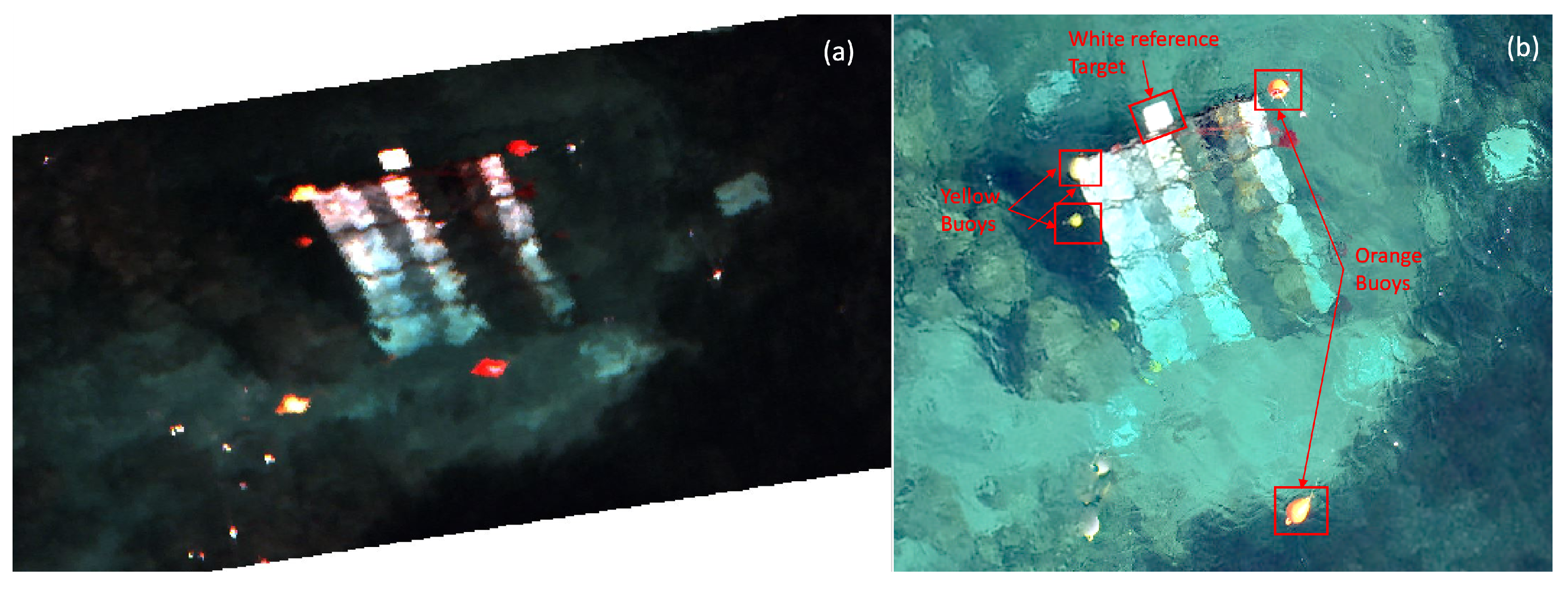
In this study, 12 hyperspectral cubes were created, five captured at 25 m and seven captured from 40 m (

Table 1. All hyperspectral cubes created for all days and heights of data acquisition.

Day No	Date	Flight Height in Meters	Georeferenced Hypercube Name	Normalized Georeferenced Hypercube Name
1	27/05/2021	40	20210527-F16-H40	20210527-F16-H40-NORM
2	28/05/2021	40	20210528-F20-H40	20210528-F20-H40-NORM
3	03/06/2021	25	20210603-F32-H25	20210603-F32-H25-NORM
4	03/06/2021	40	20210603-F31-H40	20210603-F31-H40-NORM
5	08/06/2021	25	20210608-F34-H25	20210608-F34-H25-NORM
6	08/06/2021	40	20210608-F35-H40	20210608-F35-H40-NORM
7	11/06/2021	25	20210611-F38-H25	20210611-F38-H25-NORM
8	11/06/2021	40	20210611-F42-H40	20210611-F42-H40-NORM
9	15/06/2021	25	20210615-F47-H25	20210615-F47-H25-NORM
10	15/06/2021	40	20210615-F45-H40	20210615-F45-H40-NORM
11	18/06/2021	25	20210618-F48-H25	20210618-F48-H25-NORM
12	18/06/2021	40	20210618-F49-H40	20210618-F49-H40-NORM

). An example of a hypercube of the target is presented in Figure 1. In this example, the flying altitude of the drone was 25 m above sea level. In Figure 1, it is important to point out the water surface target on the northern part of the image (white reference target from Teflon above the water surface), the large surface yellow buoys on the western part of the image, the large surface orange buoys on the eastern part, and the yellow-orange buoys (mainly underwater targets) next to the sides of the underwater target.

Spectral Measurements- Reflectance Results

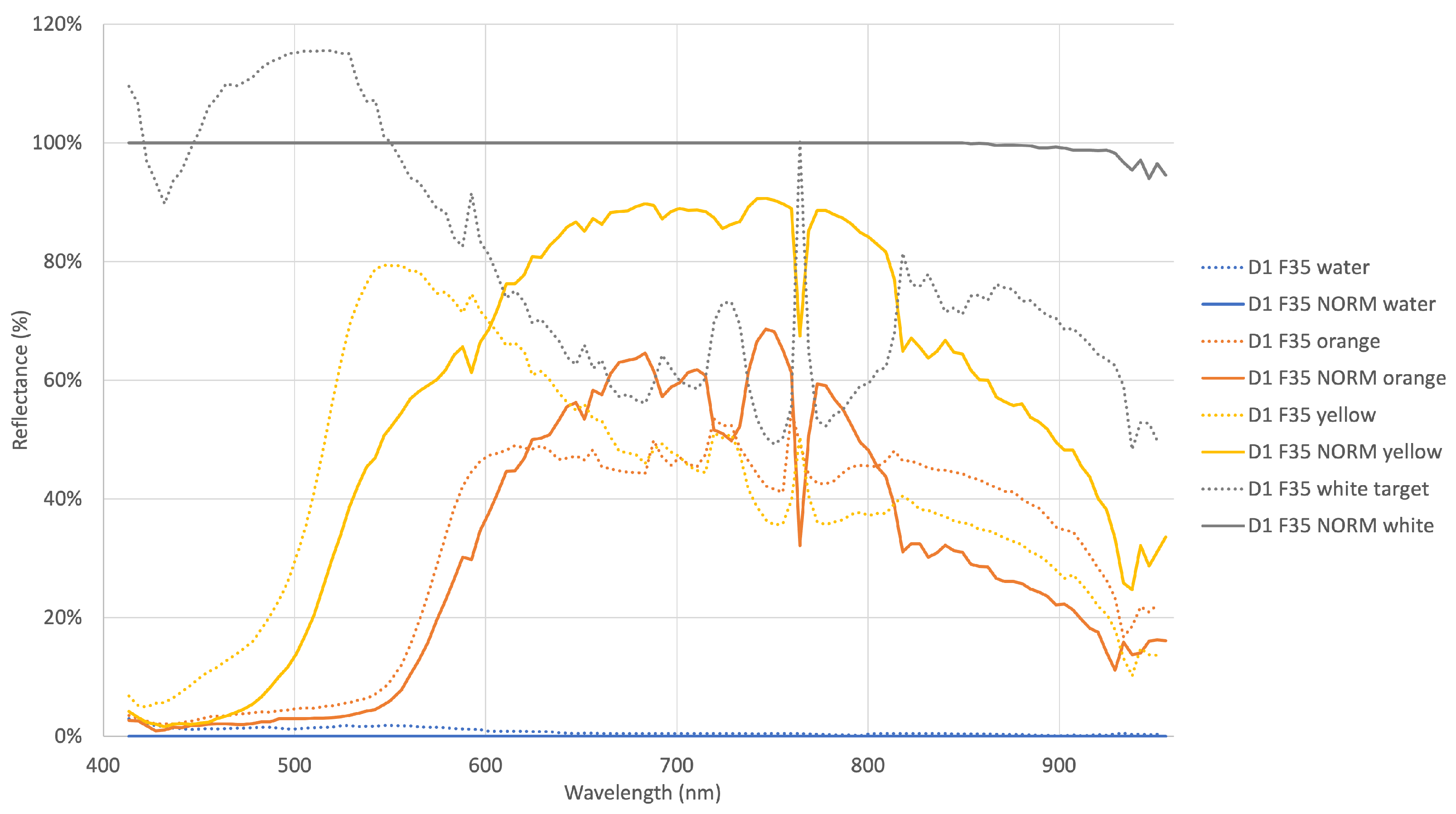
BaySpec’s hyperspectral sensor has to be calibrated radiometrically before each flight. The calibration is performed using a white reference plate provided by BaySpec with 93% reflectance, while dark reference is acquired automatically by the sensor with the shutter closed. The white and dark reference values are stored as metadata within the BaySpec’s image acquisition files and used to calculate the reflectance values by the BaySpec’s Cube Creator software. The reflectance spectral signatures of the reference targets above the water (white Teflon, orange, and yellow buoys), which were extracted from the BaySpec imagery, were compared with relevant in situ reflectance measurements, which were made using a Spectral Evolution PSR3500+ spectroradiometer. 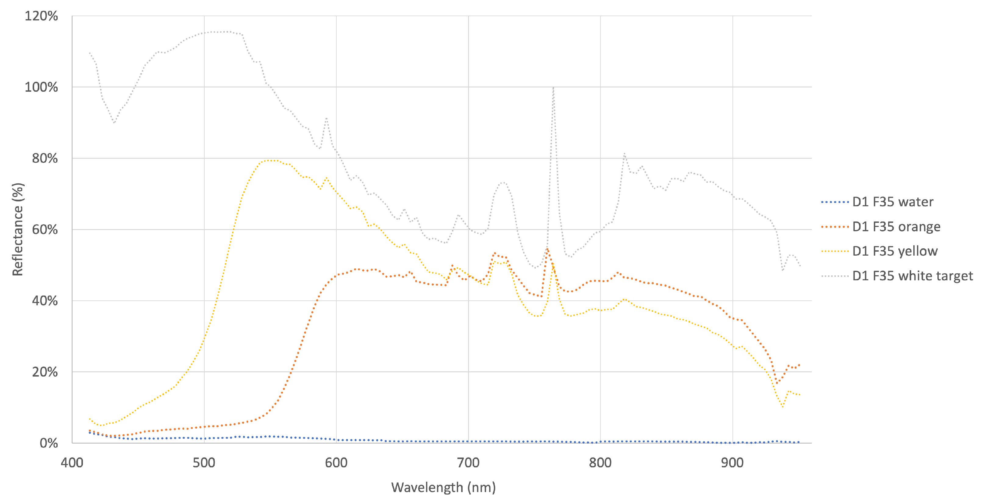The imagery-based reference measurements were carried out twice on two separate days to exclude possible errors due to natural light differences and are shown in Figure 2 and Figure 3 (dashed lines). The PSR3500+ reference in situ measurements of the surface targets are presented in Figure 4. When comparing the spectral signatures of the reference targets, we encountered several mismatches, especially for the white reference Teflon target (Figure 2, white target), which should typically have a constant flat shape around 85–95% of reflectance. Moreover, unexpected peaks around 760 nm for the reference orange and yellow buoys were observed. Therefore, we performed another radiometric calibration procedure on the raw BaySpec imagery using the Teflon plate as a white reference and some very deep-water pixels as a dark reference. The resulting normalized spectral signatures extracted from the newly calibrated imagery are presented in Figure 2 and Figure 3 (continuous lines pointed as NORM). Despite the exaggeration in the scale of the reflectance values, the newly calibrated spectral signatures of the NORM targets match the reference measurements made from the PSR3500+ spectroradiometer far better. Therefore, this type of radiometric calibration has been adopted for processing.

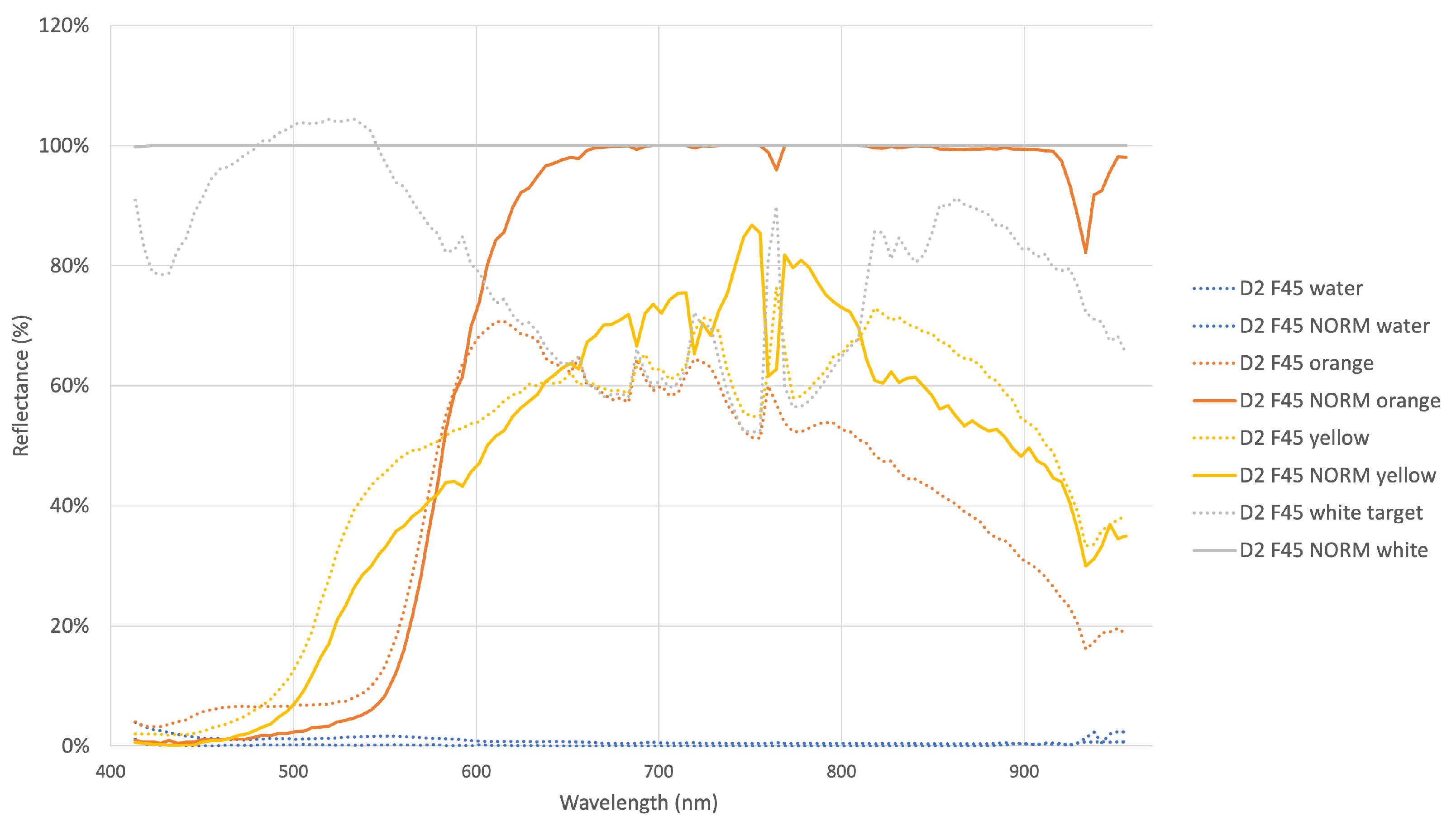
The normalized spectral signatures of Figure 2 and Figure 3 (NORM) have a normal shape from HDPE plastic. The difference in the reflectance is due to the color change, with yellow being brighter compared to orange and therefore having higher reflectance. In Figure 2 (8 June 2021), reflectance increases from 450 nm to 650 nm, where it remains relatively stable. There is a valley close to 760 nm and then a decrease from 770 to 950 nm. The same structure remains in Figure 3 (15 June 2021); however, the orange buoy presents unexpectedly high reflectance values at wavelengths higher than 600 nm. A suggested explanation of this effect is the direct light reflected from the buoy to the hyperspectral sensor due to the round shape of the buoy. This also indicates that sun glint conditions can severely impact the shape of spectral signatures, complicating the identification of the underlying material.

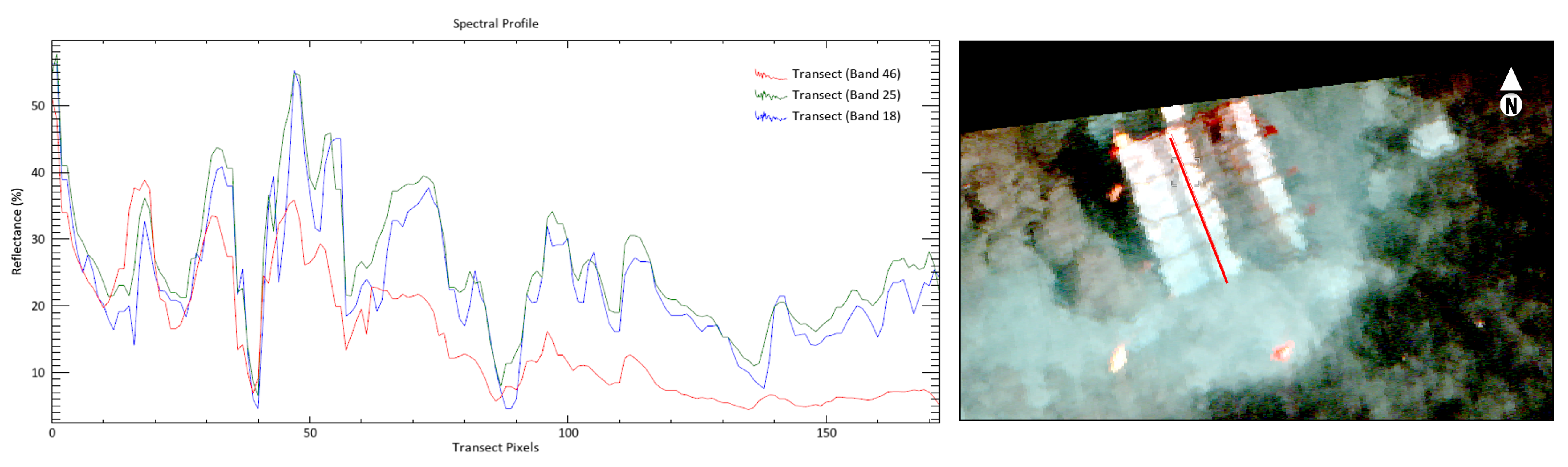
Our measurements aim to extract information about the reflectance changes due to the water depth of the different plastics. An example is illustrated in Figure 5, where RGB bands spectral signatures (Red 624.35 nm (band 46), Green 528.53 nm (band 25), Blue 426.41nm (band 18)) of PET are shown. The transect starts some cm under the water surface and ends at 3 m depth. Although single spectral transects cannot be used to derive concrete conclusions, we observe the expected attenuation of the light in all bands. Several picks should be further investigated; however, these are expected due to waves, sun glint, or plastic gaps in the structure frame. Spectral reflectance of 40% in some cm under the water is considered relatively high, which confirms the data quality, and the 5% reflectance of the red band is expected in the 3 m depth. An extensive time-series analysis is needed to examine the spectral change behavior of the plastics for the 0–3 m acquisitions. Moreover, environmental conditions (time of acquisition, wind, waves, and water clarity) must be taken into consideration for extracting a meaningful conclusion. Finally, hyperspectral lab measurements should be considered for harmonizing the spectral behavior of submerged plastics in different water depths.

3. Materials and Methods

3.1. Study Area

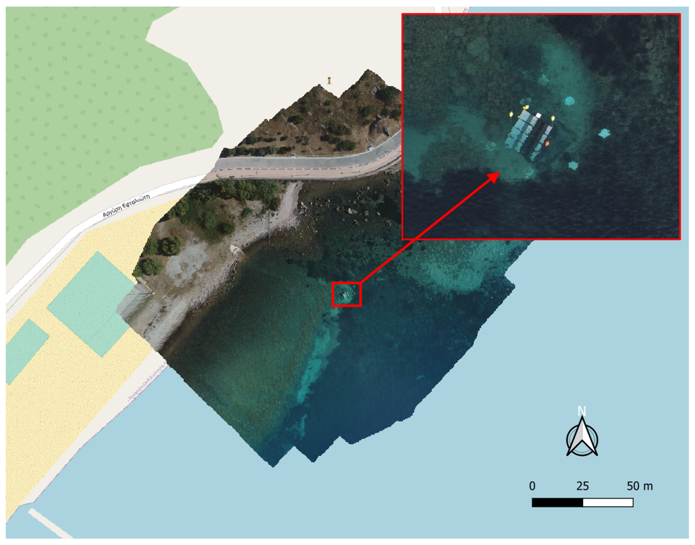
The site selected to run this experiment was Tsamakia beach, close to Mytilene city on the southeast side of Lesvos Island. This site was selected due to its bathymetry and its seabed characteristics. The water deepens gradually, reaching the necessary depth of about 3 m at a short distance from the shore, making it ideal for easy approach and target deployment and maintenance.

The seabed substrate is sandy, with rocky formations and sparse seagrass meadows, which become denser at bigger depths. Additionally, the site was selected due to its proximity to the University of the Aegean and the beach’s southeast orientation, as it is well protected from strong north and northeast winds. Figure 6 depicts the target position on Tsamakia beach.

The target was placed at about 40 m from the shoreline, on a sandy substrate, at a depth of 3.1 m. Close to the target, seagrass meadows exist and are visible as dark patches. The seagrass proved useful as a dark reference for the hyperspectral data collected during the experiment.

3.2. Methodology

3.2.1. Target Construction

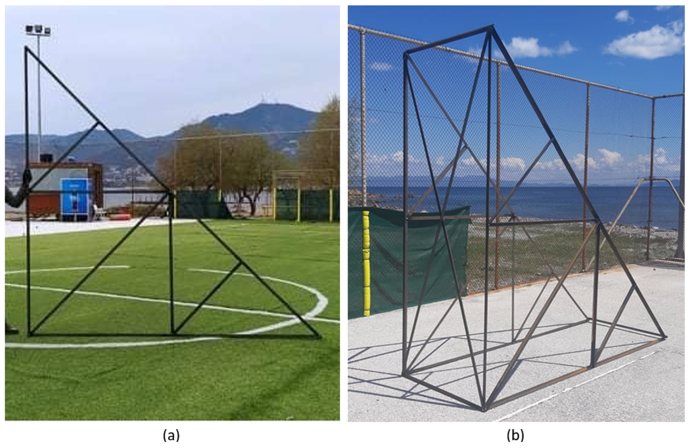
The underwater target was designed as a modular, truss-type structure, constructed using 6 m long L-section galvanized steel rails of 3 mm wall thickness, cut to the desired lengths. The design consisted of two separate target frames connected during underwater deployment to form the complete target structure. Each target frame consisted of two 3 m high simple truss members (Figure 7a), connected with parallel beams of 1.2 m in length. These parallel beams form the base to which the target materials were attached, creating slots where the target material panels were securely fixed. All connections between the L-section beams were pinned connections using 6 mm hex-type bolts. The target material panels were attached to the frame using thinner 4 mm bolts to reduce the cross-sectional area of the holes and avoid the cracking of the panels. This truss-type design and the specific L-section beams were selected to fulfill a set of distinct criteria. Firstly, the sections needed to provide enough rigidity so as for the truss-type frame to sustain the self-weight of the structure and the external loading from the current and wave action. The target material panels were not of considerable weight, but they drastically increased the surface area of the target structure. Consequently, the resultant forces on the target frame due to wave and current action were substantial. The rigidity of the structure also ensures that these external forces would be confronted with minimal frame deformation to avoid damage of the target panels due to bending. Secondly, the design of the target frame fulfills the criterion of overall weight and maneuverability, both on land and in water. The overall structure of the target allows it to be handled by a relatively small number of people, moved into the water, and deployed underwater by an underwater team of three people. Finally, the target is designed to be constructed without the the use of specialized equipment or personnel and to allow for easy disassembly and storage.

The field test target design consists of the following components:

• A truss structure to support a 45-degree slope down into the water. The structure’s height is 3 m (Figure 8a),
• A dark background sail (Figure 8b),
• A depth/distance gauge made by alternating black/white patches. In the first meter, the gauge has a resolution of 10 cm. The second and third meters it has a resolution of 20 cm. The final and deepest part has a resolution of 50 cm. This gauge can be observed in Figure 8c.
• Eight sample materials, mounted as 30 cm wide strips and running down the slope (in the order on the target left to the right):
  • PP (5 mm thickness);
  • PA-6 (5 mm thickness);
  • PVC (5 mm thickness);
  • White PS (10 mm thickness);
  • PET (5 mm thickness);
  • Black HDPE (5 mm thickness);
  • XPS (5 mm thickness);
  • LDPE, sourced from white plastic bags (<1 mm thickness).
• Two sample object types at 1 m depth intervals: yellow HDPE buoys on one side, red PA6 net balls on the other side,
• A 30 × 30 cm white reference plate, made of PTFE, mounted horizontally, such that it is always above water level. This reference plate can be observed in the top view in Figure 8d.

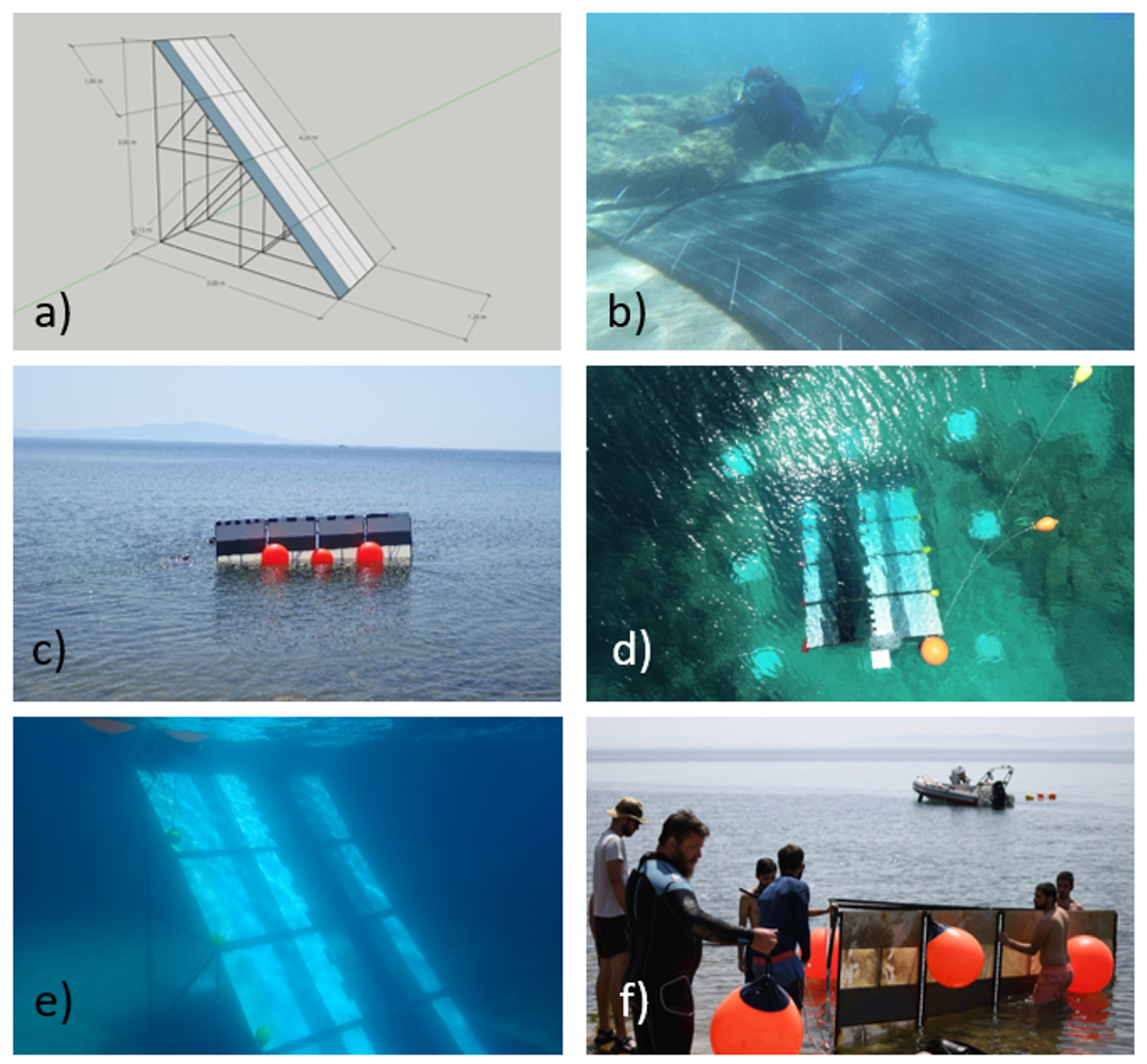
Figure 8 illustrates the deployment phase and gives an overview of the actions made during the target’s placement. Figure 8e shows the target just after submersion. From 25 May 2021, the target has remained deployed until 18 June 2021. As shown in Figure 8f, the target has gathered a significant amount of biofouling during the deployment period. The ground team regularly checked the target state and position and adjusted it accordingly during the entire deployment. Passing ferry ships or extreme weather conditions have occasionally moved the target away from its dark background, and additional adjustment was necessary. Thus, a diving team deployed extra weight to keep the target in position. Overall, the target stayed intact and was positioned very well during the 3-week deployment period.

3.2.2. Data Collection

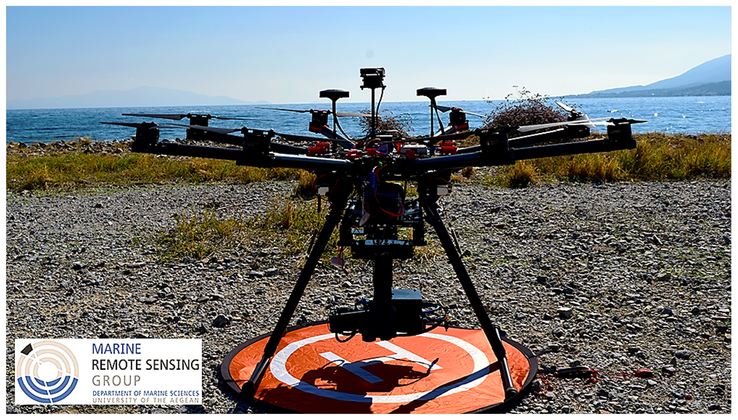
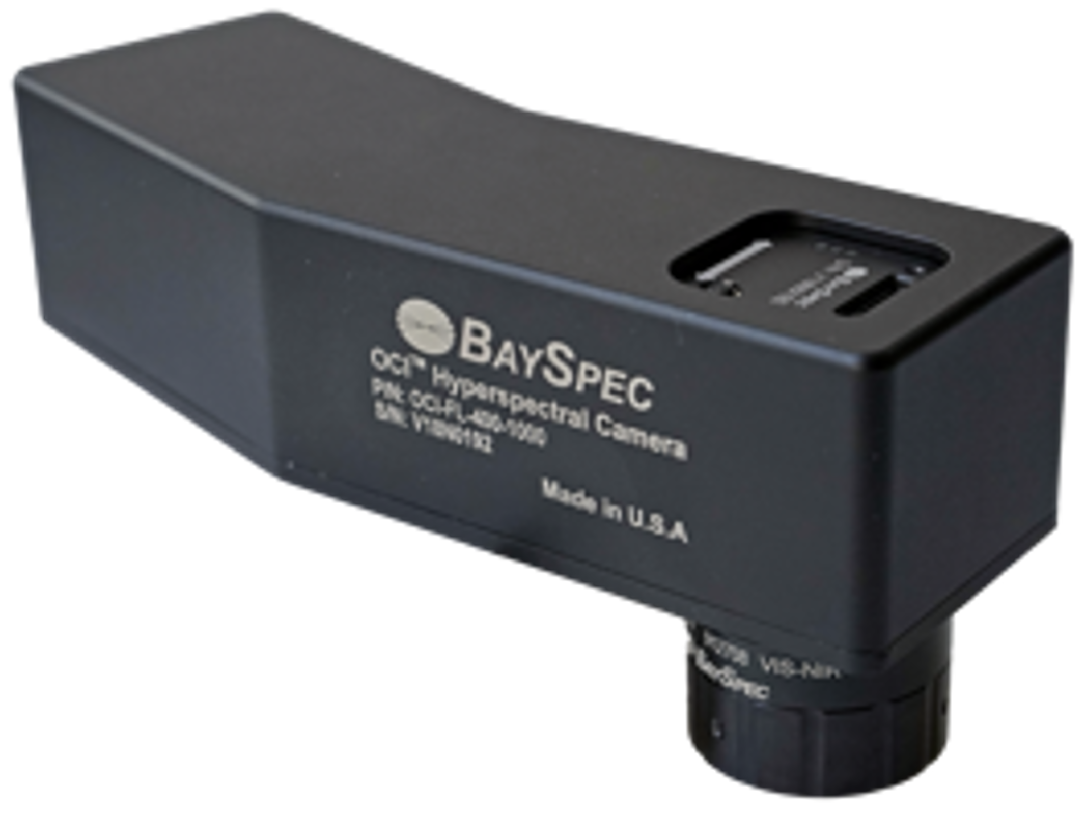
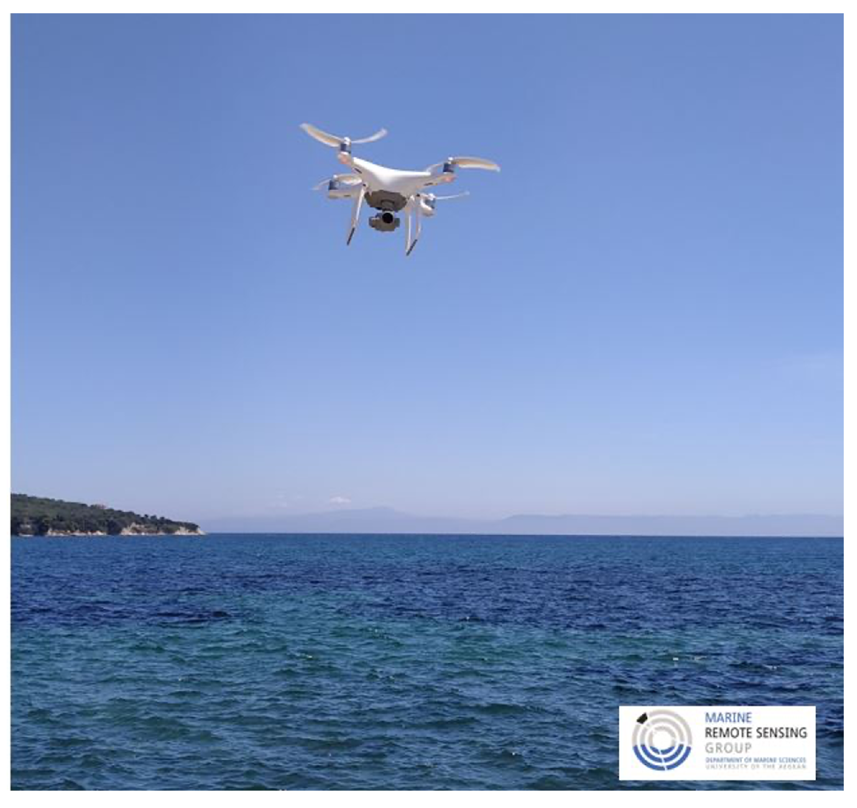
The data collection was realized from the 26th of May until the 18th of June. The team used two Unmanned Aerial Vehicles (UAVs). The first UAV was a customized DJI S1000 octocopter (Figure 9) to carry the hyperspectral push-broom sensor (Figure 10). The second UAV was a DJI Phantom 4 Pro v2 (Figure 11) for obtaining high-resolution RGB orthomosaics, which aided the hyperspectral data georeferencing and helped monitor the target’s condition and position.

The hyperspectral camera used for this experiment was the OCI-F Imager, created by BaySpec Inc. [16]. OCI-F is a miniaturized push-broom type hyperspectral camera covering the full VIS-NIR (400–1000 nm) wavelength range in 121 spectral bands with a width of 5–7 nm, specifically designed for UAV monitoring applications. It features ultra-compactness (14 cm × 7 cm × 7 cm) and is lightweight (570 g) with fast data transfer rates (up to 60 fps). The lens size is 16mm (19.3° FOV), and the spatial pixels have a range of 800 px × scan length. Marine Remote Sensing Group uses the camera, as it offers versatility on airborne platforms such as UAVs and provides hyperspectral image stitching. It is ideal for applications such as remote sensing and all airborne applications such as marine litter detection and coastal mapping.

The hyperspectral camera was mounted on a custom-made UAV. The airframe is based on the DJI S1000 Frame, an octocopter having the following specifications: (i) empty weight of 5.1 Kg, (ii) diameter of 0.8 m, and (iii) 5 Kg payload capacity. A custom, two-axis gimbal was created for the camera to be mounted to the UAV frame. The gimbal was tailor-made to handle sensor yaw and pitch and stabilize the camera level to nadir when acquiring data. The system’s total weight was 8.2 kg and was capable of 15 min of airtime. The UAS used in this experiment is depicted in Figure 9.

The OCI-F hyperspectral sensor used to realize the experiment is a true push--broom imager not dependent on a constant scanning speed. It was decided that the UAV data acquisition process scans the target vertically and inline aligned. Thus, achieve the best possible alignment (vertically and inline) between the material stripes and the pushbroom scan stripes of the imager. The Ardupilot Mission Planner software [17] was used to create the different approaches to the automatic flight planning tested.

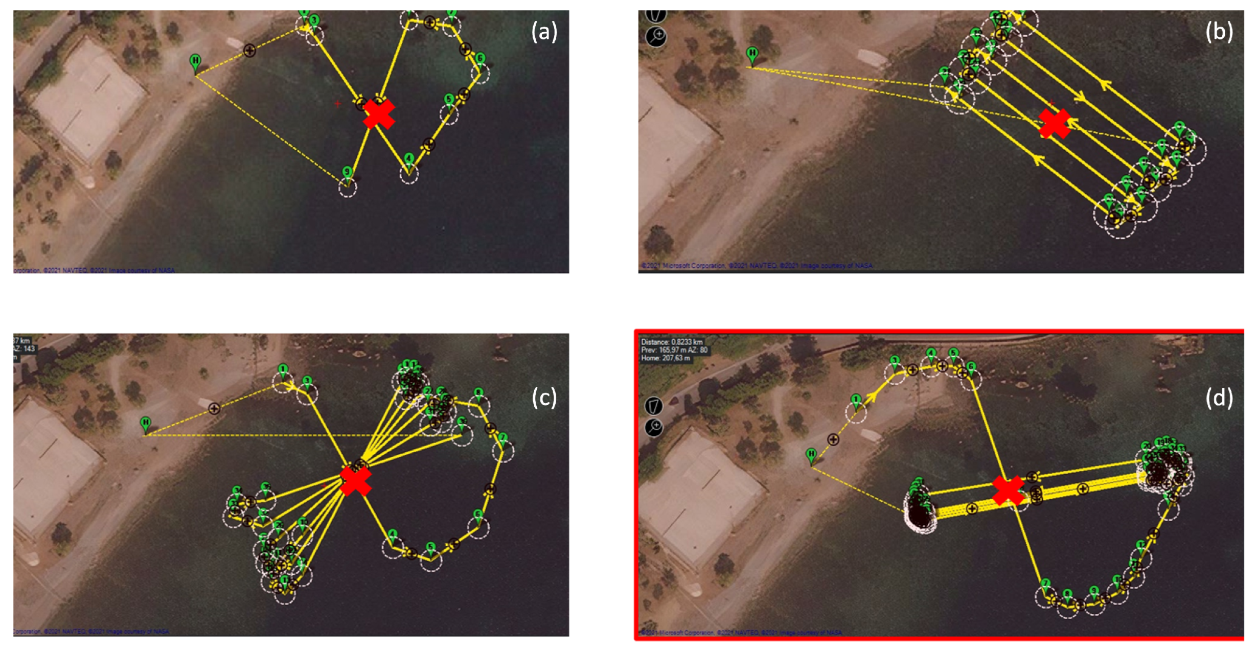
Several iterations and test flights with varying flight line patterns (Figure 12) were required. Finally, after optimizing the flight line bearing, the most effective flight path was a collection of densely packed parallel flight lines vertically placed above the horizontal axes of the targets (Figure 12d—bottom right mission depicts the optimal flight path).

All flight attempts were realized from the 26th of May until the 18th of June (

Table 2. All Flight missions that took place for the realization of the experiment.

No	Date	Flight Time Window	Number of Flights	Weather (Cloud Cover%, Temperature, Humidity%)	Mission Type
1	26/05/2021	09:12–10:04	3	22%, 23C, 59%	Flight Pattern & Camera Parameterization
2	27/05/2021	10:15–11:05	3	24%, 22C, 74%	Data Collection
3	28/05/2021	08:03–10:40	8	56%, 21C, 88%	Data Collection
4	01/06/2021	18:12–19:32	5	20%, 22C, 52%	Data Collection
5	03/06/2021	10:04–12:10	4	5%, 19C, 64%	Data Collection
6	08/06/2021	08:10–10:35	3	20%, 23C, 73%	Data Collection
7	11/06/2021	09:31–11:29	6	0%, 23C, 68%	Data Collection
8	15/06/2021	10:15–11:41	5	67%, 20C, 65%	Data Collection
9	18/06/2021	09:20–10:28	3	0%, 24C, 74%	Data Collection

). The overall weather conditions were ideal, with temperatures ranging from 19–24 degrees Celsius, humidity from 59 to 88%, and cloud cover from 0 to 67%. The overall number of test flights was 40, and the heights for data acquisition were 25 and 40 m. The overlap used during the data acquisition for orthomosaic creation was 80% for both side and front overlaps. No mosaicing was realised for hyperspectral cube creation, as the cubes were vertically and inline aligned between the plastic material stripes of the target and the pushbroom scan stripes of the imager. The team produced hyperspectral cubes from 31 out of 40 flights and 8 out of 9 test days. Cubes were not created for nine flights, as five were realized in the afternoon with limited illumination and four on a windy day with wavy sea status causing errors in hypercube creation. The team did not manage to collect data on the 26th of May, as it was testing the most appropriate flight path. Furthermore, they experimented with the OCI-F imager parameterization on this day to define how the sensor correctly captures all the submerged targets.

3.2.3. Data Processing Methodology

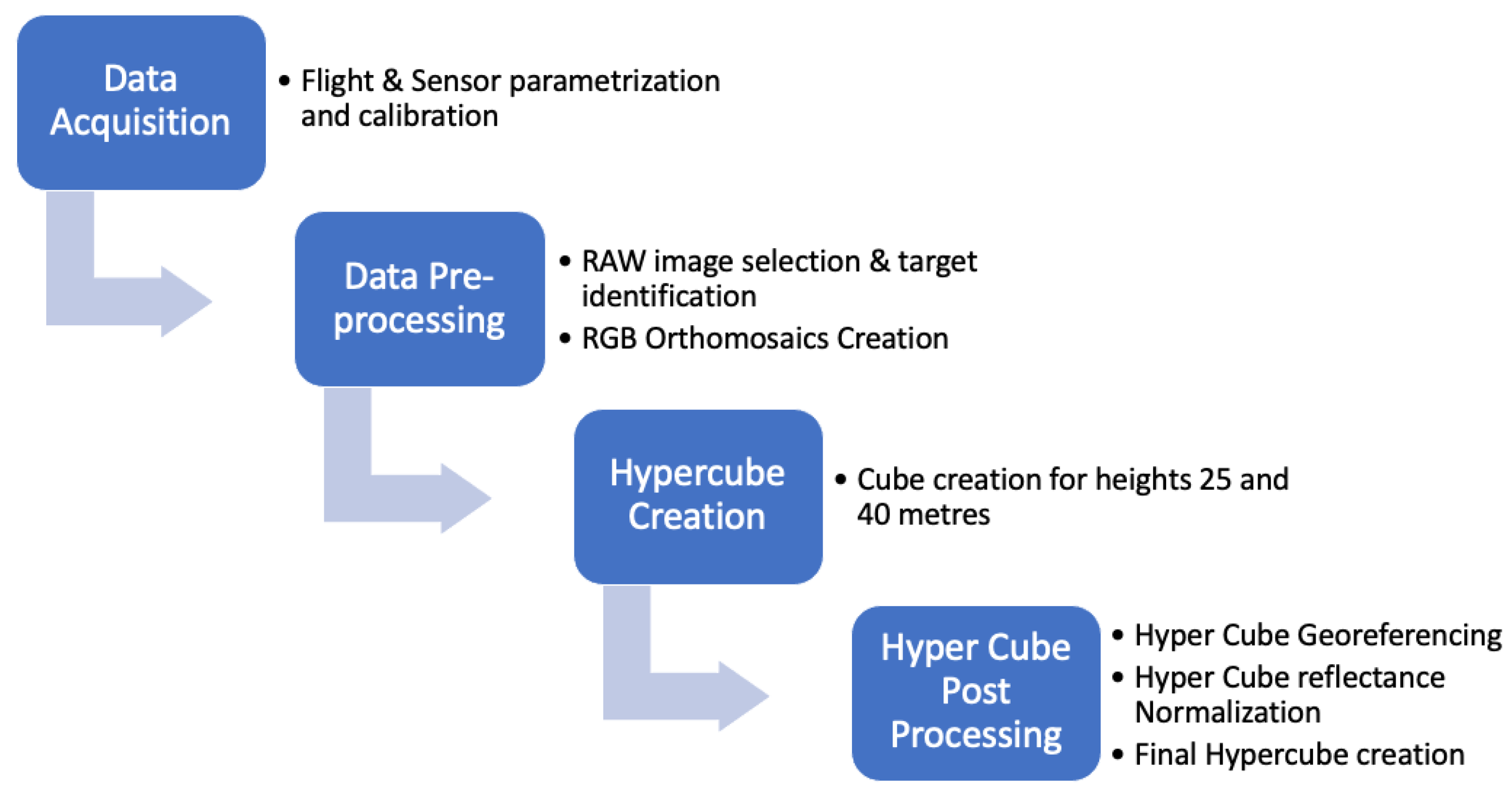
A methodological workflow was created to standardize the performance monitoring strategy for an airborne spectral reflectance dataset of submerged plastic targets in a coastal environment. The methodology is based on four pillars: The first pillar is the data acquisition protocol that enables the system selection, system preparation, mission programming, and the data acquisition flight. The second pillar consists of the preprocessing step, where an experienced photo interpreter selects the correct raw image sequences that depict the submerged target using the CubeCreator provided by BaySpec [16]. Furthermore, in this step, very high resolution RGB orthomosaics are created to be used as a base for georeferencing the hypercubes. The third pillar is the hypercube creation. Finally, the hypercubes created from the previous step were georeferenced using Q-GIS [19], and all their bands were normalized and checked for reflectance integrity errors. The following flowchart (Figure 13) illustrates the methodological steps and the overall structure of the approach proposed by this study.

The OCI-F Imager carries two sensors, one push-broom hyperspectral sensor (sensor-1) and a RGB snapshot camera (sensor-2), whose images are used for hyperspectral scan stripe stitching. During the data pre-processing step, the raw data sequence depicting the sub-merged target had to be selected. Before processing the recorded raw hyperspectral scan stripes for creating the hyperspectral cubes, the user should select the correct range of raw hyperspectral stripes from sensor-1. The image selection process is a manual interpretation process realized by an expert and is driven using RGB images from sensor-2. In this process, the photo-interpreter selected the sequence of raw hyperspectral stripes in the flight line where the drone passed exactly above the underwater target. Normally, after hyperspectral data range selection, the BaySpec’s Cube Creator software is used to create the hyperspectral cubes. Cube Creator is a Microsoft Windows-based software provided by the camera vendor. It is used to process the raw images recorded by the two camera sensors; the hyperspectral one (sensor-1) and the RGB (sensor-2). The software uses the RGB images captured by camera’s sensor-2 to match the hyperspectral sensor’s (sensor-1) data, i.e., align the hyperspectral stripes in a sequence using the RGB images as a reference, thus creating the cube. Furthermore, it allows the user to display and check the raw images, view the hyperspectral cubes in different spectral bands, display the spectra from the cube files and perform classification calculations from the spectrum data. Even though the Cube Creator software works seamlessly in most cases, when the hyperspectral image acquisitions are carried out solely over water areas, the hyperspectral lines of the sensor 1 fail to align using the RGB images of sensor-2. The software cannot locate the necessary tie points, since no regular object shapes are depicted in the images. Therefore, our team created an ANSI C routine, which created hyperspectral cubes (in 8-bit or 16-bit format, depending on the acquisition settings) directly from the selected raw OCI-F hyperspectral stripes, without geometric alignment. These hypercubes, which contained the targets, were then manually georeferenced by selecting control points from the DJI Phantom 4 RGB orthomosaics. Since the scan length over the sub-merged target is quite small and the UAV only captured a straight flight line, only minor geometric distortions were observed, and the georeferencing process (carried out in QGIS) is considered sufficient in terms of geometric accuracy. The hyperspectral cubes are depicting the plastic target at surface level with an approximate pixel size of 1 and 1.5 cm for 25 and 40 m flight heights, respectively. No corrections have been made to optically enhance the hyperspectral cubes’ resolution, as the pixels become coarser according to depth. The estimated change in resolution is less than 0.1 cm due to the small height difference of the plastic targets (3 m surface to bottom distance).

4. Conclusions

A hyperspectral dataset was created for eight submerged types of plastics using a BaySpec OCI-F hyperspectral camera. Plastics were deployed at 0–3 m depth and remained submerged for a period of three weeks. A total of 12 hyperspectral cubes were created from two different UAV flight path heights (25 and 40 m). From the present study, four main conclusions can be derived. Firstly, it is extremely challenging to couple very similar datasets due to a variety of factors occurring during the acquisition times. Water clarity-turbidity, sea waves (short gravity-capillary or swell), sea foam, and light conditions are some examples of the obstacles that need to be overcome. These in situ conditions play a significant role for the quality of the data sets.

Secondly, a correct UAV flight path over the target is crucial for the final data cubes. From our observations, we conclude that it is important to scan the submerged target vertically on the inclined side to acquire complete lines of the submerged plastics. High repeatability of the flight tracks is essential for the similarity of the data set. However, due to the GPS error of the drone’s flight controller, it is not easy to achieve the same path over the target. Therefore, every acquisition required to fly several times over the same target to scan it correctly.

Thirdly, we conclude that push broom hyperspectral scanners cannot easily be used above water surfaces. Often, the scanning lines cannot be aligned (even manually), and therefore the final image quality is questionable. This is because the water surface moves during the scanning, and the sensor cannot acquire the right illumination from the target. Additionally, the georeferencing procedure, most of the time, is problematic since the RGB sensor cannot be used correctly for the alignment of hyperspectral lines due to the dynamic behavior of the sea surface.

Fourthly, additional calibration is needed when a push broom hyperspectral scanner is used above water surfaces. Especially for targets with low sensitivity, e.g., underwater targets, some reference targets should always be present during the experiments. The quality of the hypercubes should always be examined against known reference targets, and a threshold should be applied for accepting them as appropriate for further analysis and publication.

References

- Geyer, R.; Jambeck, J.R.; Law, K.L. Production, use, and fate of all plastics ever made. Sci. Adv. 2017, 7. [Google Scholar] [CrossRef] [PubMed] [Green Version]
- Lebreton, L.; Slat, B.; Ferrari, F.; Sainte-Rose, B.; Aitken, J.; Marthouse, R.; Hajbane, S.; Cunsolo, S.; Schwarz, A.; Levivier, A.; et al. Evidence that the Great Pacific Garbage Patch is rapidly accumulating plastic. Sci. Rep. 2018, 8, 4666. [Google Scholar] [CrossRef] [PubMed] [Green Version]
- Garaba, S.P.; Aitken, J.; Slat, B.; Dierssen, H.M.; Lebreton, L.; Zielinski, O.; Reisser, J. Sensing Ocean Plastics with an Airborne Hyperspectral Shortwave Infrared Imager. Environ. Sci. Technol. 2018, 52, 11699–11707. [Google Scholar] [CrossRef] [PubMed]
- Evans, M.C.; Ruf, C.S. Toward the Detection and Imaging of Ocean Microplastics with a Spaceborne Radar. IEEE Trans. Geosci. Remote Sens. 2022, 60, 4202709. [Google Scholar] [CrossRef]
- De Vries, R.; Egger, M.; Mani, T.; Lebreton, L. Quantifying floating plastic debris at sea using vessel-based optical data and artificial intelligence. Remote Sens. 2021, 13, 3401. [Google Scholar] [CrossRef]
- Ciappa, A.C. Marine plastic litter detection offshore Hawai’i by Sentinel-2. Mar. Pollut. Bull. 2021, 168, 112457. [Google Scholar] [CrossRef] [PubMed]
- Topouzelis, K.; Papakonstantinou, A.; Garaba, S.P. Detection of floating plastics from satellite and unmanned aerial systems (Plastic Litter Project 2018). Int. J. Appl. Earth Obs. Geoinf. 2019, 79, 175–183. [Google Scholar] [CrossRef]
- Garaba, S.P.; Arias, M.; Corradi, P.; Harmel, T.; de Vries, R.; Lebreton, L. Concentration, anisotropic and apparent colour effects on optical reflectance properties of virgin and ocean-harvested plastics. J. Hazard. Mater. 2021, 406, 124290. [Google Scholar] [CrossRef] [PubMed]
- Diruit, W.; Le Bris, A.; Bajjouk, T.; Richier, S.; Helias, M.; Burel, T.; Lennon, M.; Guyot, A.; Ar Gall, E. Seaweed Habitats on the Shore: Characterization through Hyperspectral UAV Imagery and Field Sampling. Remote Sens. 2022, 14, 3124. [Google Scholar] [CrossRef]
- Harishidayat, D.; Al-Shuhail, A.; Randazzo, G.; Lanza, S.; Muzirafuti, A. Reconstruction of Land and Marine Features by Seismic and Surface Geomorphology Techniques. Appl. Sci. 2022, 12, 9611. [Google Scholar] [CrossRef]
- Tasseron, P.; van Emmerik, T.; Peller, J.; Schreyers, L.; Biermann, L. Advancing floating macroplastic detection from space using experimental hyperspectral imagery. Remote Sens. 2021, 13, 2335. [Google Scholar] [CrossRef]
- Freitas, S.; Silva, H.; Silva, E. Remote hyperspectral imaging acquisition and characterization for marine litter detection. Remote Sens. 2021, 13, 2536. [Google Scholar] [CrossRef]
- Knaeps, E.; Sterckx, S.; Strackx, G.; Mijnendonckx, J.; Moshtaghi, M.; Garaba, S.P.; Meire, D. Hyperspectral-reflectance dataset of dry, wet and submerged marine litter. Earth Syst. Sci. Data 2021, 13, 713–730. [Google Scholar] [CrossRef]
- Kooi, M.; Reisser, J.; Slat, B.; Ferrari, F.F.; Schmid, M.S.; Cunsolo, S.; Brambini, R.; Noble, K.; Sirks, L.A.; Linders, T.E.; et al. The effect of particle properties on the depth profile of buoyant plastics in the ocean. Sci. Rep. 2016, 6, 33882. [Google Scholar] [CrossRef] [PubMed] [Green Version]
- Law, K.L.; Morét-Ferguson, S.E.; Goodwin, D.S.; Zettler, E.R.; Deforce, E.; Kukulka, T.; Proskurowski, G. Distribution of surface plastic debris in the eastern pacific ocean from an 11-year data set. Environ. Sci. Technol. 2014, 48, 4732–4738. [Google Scholar] [CrossRef] [PubMed]
- BaySpec. OCI™-F Hyperspectral Imager (VIS-NIR, SWIR)-BaySpec. 2022. Available online: https://www.bayspec.com/spectroscopy/oci-f-hyperspectral-imager/ (accessed on 1 December 2022).
- ArduPilot. Mission Planner. 2019. Available online: http://ardupilot.org/planner/docs/mission-planner-overview.html (accessed on 1 December 2022).
- Google. Google Maps. 2022. Available online: https://www.google.com/maps/ (accessed on 1 December 2022).
- QGIS Development Team. QGIS Geographic Information System; Open Source Geospatial Foundation: Beaverton, OR, USA, 2022. [Google Scholar]
Figure 1.
Depiction of the target from an altitude of 25 m: (a) RGB image of the hyperspectral cube using three channels; (b) RGB orthomosaic.
Figure 2.
Spectral signatures derived from the hyperspectral cube for 8 June 2021 (Flight number 35–height 40 m).
Figure 3.
Spectral signatures derived from the hyperspectral cube for 15 June 2021 (Flight number 45–height 40 m).
Figure 4.
Diagram of spectra for reference targets derived from PSR3500+ spectroradiometer in situ measurements.
Figure 5.
Transect plot of hypercube 11 June 2021 for RGB bands (Flight number: 38, height 25 m).
Figure 6.
Orthomosaic, indicating the placement of the target in Tsamakia beach. The red outlined inset is a close-up view of the target and the substrate of the sea bottom. Basemap is provided by OSM ((OpenStreetMap (OSM)).
Figure 7.
(a) A single truss member of the target frame structures, (b) one of the two single-target frames before the parallel beams are attached.
Figure 8.
(a) Technical draft of one-half of the target, (b) dark background being deployed by the team of divers, (c) the target being deployed using flotation balloons, (d) close-up top view of the target, (e) the submerged target, just after deployment, and (f) the target being decommissioned after three weeks. Biofouling is visible.
Figure 9.
DJI S1000 with Bayspec OCI-F on a custom-made gimbal.
Figure 10.
BaySpec OCI-F hyperspectral push-broom sensor [
16].
Figure 11.
DJI Phantom 4 Pro v2 UAV.
Figure 12.
All tested flights have different patterns to achieve the best coverage of the target. Attempted data acquisition flight patterns (
a) x shaped, (
b) grid path, (
c) multi-x shaped with various angles. Subfigure (
d) depicts closely aligned parallel flight lines that proved to be the most effective. Using this flight pattern, the entire target was scanned in one pass, depicting the target in one hyperspectral cube. Basemaps are provided by Google [
18].
Figure 13.
Methodological workflow.