
Determining Plant Diversity within Interconnected Natural Habitat Remnants (Ecological Network) in an Agricultural Landscape: A Matter of Sampling Design?

 ,
,  , ,
, ,  and
and 
Abstract
:1. Introduction
2. Materials and Methods
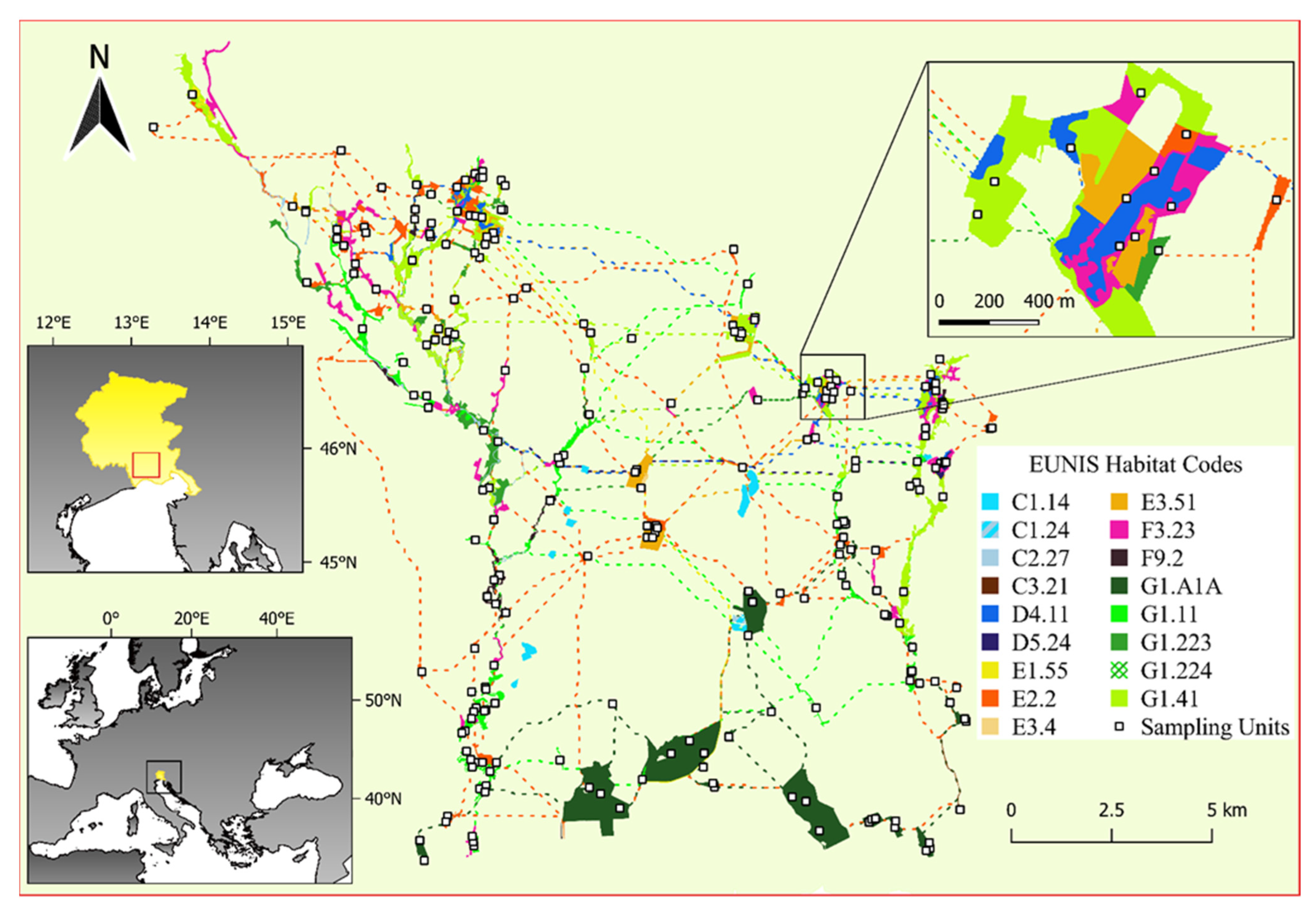
2.1. Study Area and EN Model
2.2. Sampling Design and Data Collection within the EN
2.3. Data Analysis
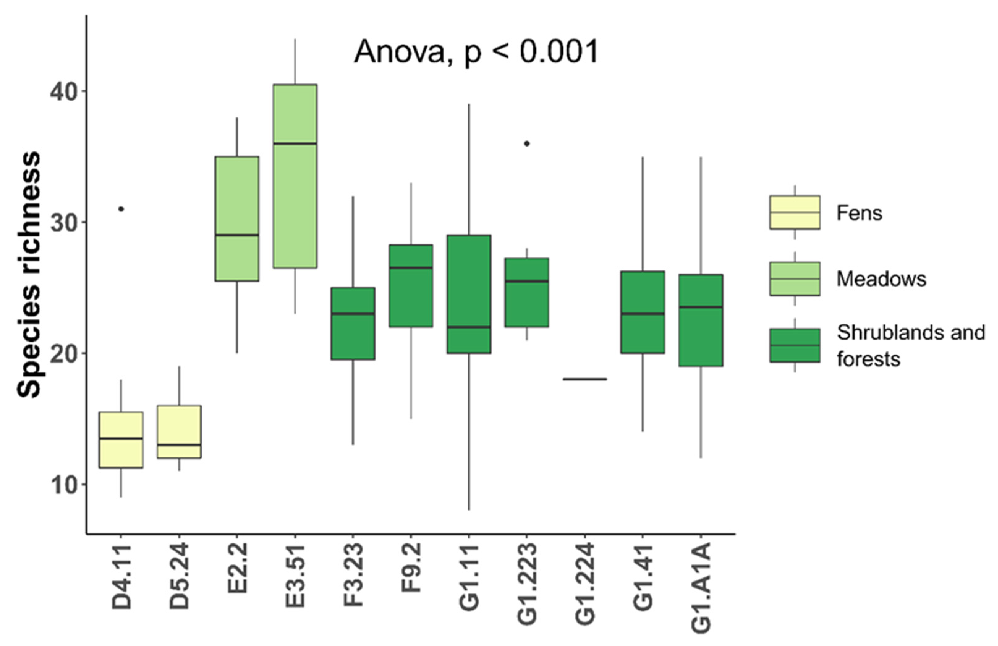
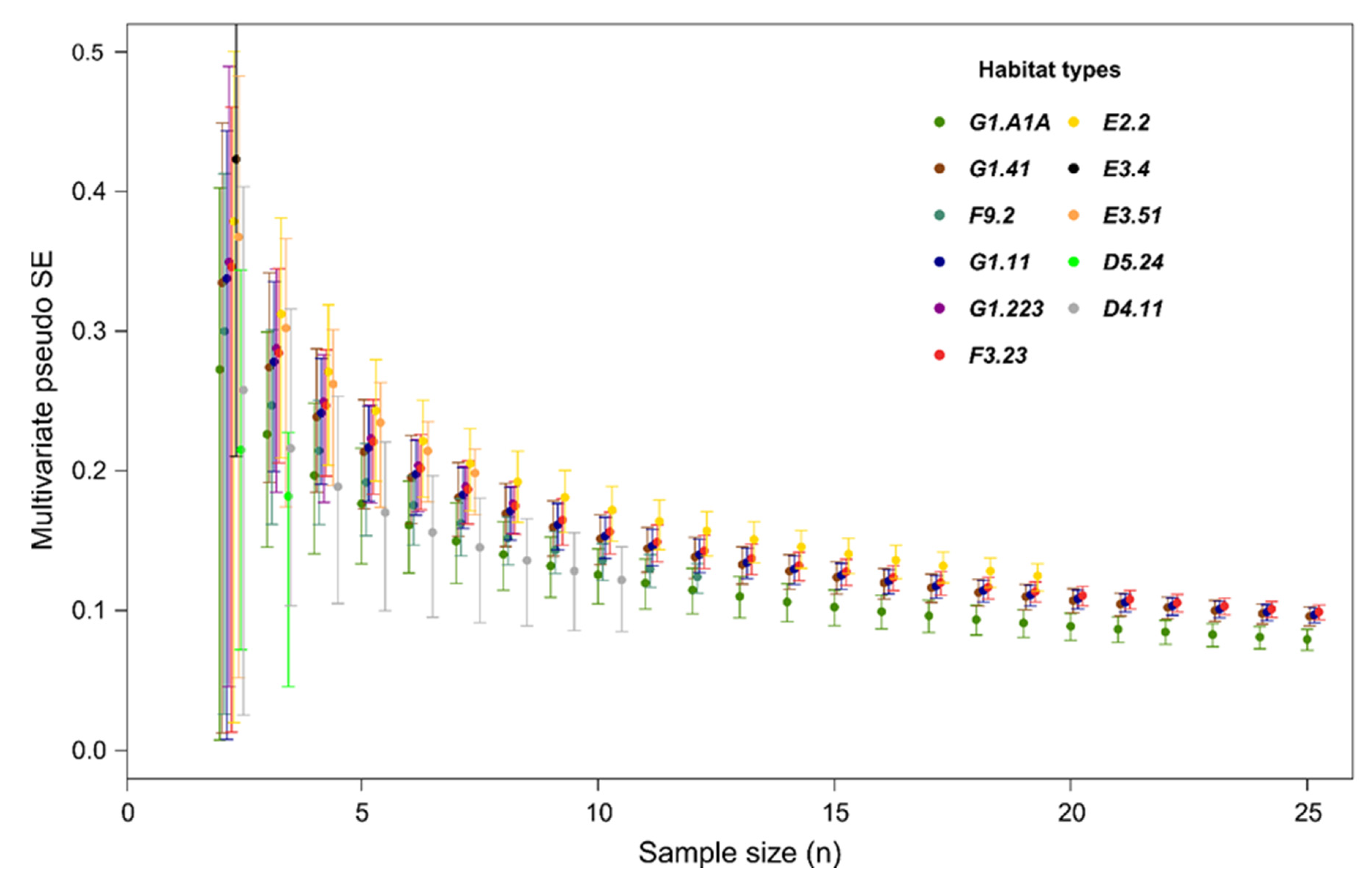
3. Results
4. Discussion
5. Conclusions
Supplementary Materials
Author Contributions
Funding
Institutional Review Board Statement
Informed Consent Statement
Data Availability Statement
Acknowledgments
Conflicts of Interest
References
- Landi, P.; Minoarivelo, H.O.; Brännström, Å.; Hui, C.; Dieckmann, U. Complexity and stability of ecological networks: A review of the theory. Popul. Ecol. 2018, 60, 319–345. [Google Scholar] [CrossRef]
- IPBES. Summary For Policymakers of the Global Assessment Report on Biodiversity and Ecosystem Services of the Intergovernmental Science-Policy Platform on Biodiversity and Ecosystem Services; Díaz, S., Settele, J., Brondízio, E.S., Ngo, H.T., Guèze, M., Agard, J., Arneth, A., Balvanera, P., Brauman, K.A., Butchart, S.H.M., et al., Eds.; IPBES: Bonn, Germany, 2019; p. 56. [Google Scholar] [CrossRef]
- EEA. State of Nature in the EU Report European Environment Agency 2020. State of Nature in the EU. Results from Reporting under the Nature Directives 2013–2018; Publication office of European Unions: Luxembourg, 2020; p. 142. ISBN 978-92-9480-259-0. [Google Scholar] [CrossRef]
- UN (United Nation). Transforming our World: The 2030 Agenda for Sustainable Development, A/RES/70/L.1. Resolution Adopted by the General Assembly; United Nations: New York, NY, USA, 2015; Available online: https://sustainabledevelopment.un.org/post2015/transformingourworld/publication (accessed on 12 November 2021).
- UN (United Nations). Sustainable Development Goals; United Nations: New York, NY, USA, 2015; Available online: http://www.un.org/sustainabledevelopment/sustainable-development-goals/ (accessed on 12 November 2021).
- European Commission. Communication from the Commission to the European Parliament, the Council, the European Economic and Social Committee and the Committee of the Regions EU Biodiversity Strategy for 2030 Bringing Nature Back into Our Lives COM/2020/380 Final 20.5.2020 Brussels 2020. Available online: https://eur-lex.europa.eu/legal-content/EN/TXT/?uri=CELEX:52020DC0380 (accessed on 16 November 2021).
- Cushman, S.A.; McRae, B.; Adriaensen, F.; Beier, P.; Shirley, M.; Zeller, K. Biological corridors and connectivity. In Key Topics in Conservation Biology 2; Macdonald, D.W., Willis, K.J., Eds.; Wiley-Blackwell: Hoboken, NJ, USA, 2013; pp. 384–404. [Google Scholar]
- Pascual, M.; Dunne, J. Ecological Networks: Linking Structure to Dynamics in Food Webs; Oxford University Press: New York, NY, USA, 2006. [Google Scholar]
- Fahrig, L. Effects of habitat fragmentation on biodiversity. Annu. Rev. Ecol. Evol. Syst. 2003, 34, 487–515. [Google Scholar] [CrossRef] [Green Version]
- Battisti, C. Frammentazione Ambientale Connettività Reti Ecologiche: Un Contributo Teorico E Metodologico Con Particolare Riferimento Alla Fauna Selvatica; Provincia di Roma Assessorato alle Politiche Agricole, Ambientali e Protezione Civile: Rome, Italy, 2004. (In French) [Google Scholar]
- Biondi, E.; Nanni, L. Geosigmeti, Unità Di Paesaggio E Reti Ecologiche. In Identificazione E Cambiamenti Nel Paesaggio Contemporaneo; Blasi, C., Paolella, A., Eds.; Atti del Terzo Congresso IAED: Roma, Italy, 2005; pp. 134–140. [Google Scholar]
- Rosati, L.; Fipaldini, M.; Marignani, M.; Blasi, C. Effects of fragmentation on vascular plant diversity in a Mediterranean forest archipelago. Plant. Biosyst. 2010, 144, 38–46. [Google Scholar] [CrossRef]
- Forman, R.T.T. Land Mosaics; Cambridge University Press: Cambridge, UK, 1995. [Google Scholar]
- Foltête, J.C. How ecological networks could benefit from landscape graphs: A response to the paper by Spartaco Gippoliti and Corrado Battisti. Land Use Policy 2019, 80, 391–394. [Google Scholar] [CrossRef]
- Tischendorf, L.; Fahrig, L. On the usage and measurement of landscape connectivity. Oikos 2000, 90, 7–19. [Google Scholar] [CrossRef] [Green Version]
- Taylor, P.D.; Fahrig, L.; With, K.A. Landscape connectivity: A return to the basics. In Connectivity Conservation; Cambridge University Press: Cambridge, UK, 2006. [Google Scholar]
- Taylor, P.D.; Fahrig, L.; Henein, K.; Merriam, G. Connectivity is a vital element of landscape structure. Oikos 1993, 68, 571–573. [Google Scholar] [CrossRef] [Green Version]
- LaPoint, S.; Balkenhol, N.; Hale, J.; Sadler, J.; van Der Ree, R. Ecological connectivity research in urban areas. Funct. Ecol. 2015, 29, 868–878. [Google Scholar] [CrossRef]
- Damschen, E.I. Landscape Corridors. In Encyclopedia of Biodiversity, 2nd ed.; Levin, S.A., Ed.; Academic Press: Cambridge, MA, USA, 2013; pp. 467–475. [Google Scholar] [CrossRef]
- De Montis, A.; Caschili, S.; Mulas, M.; Modica, G.; Ganciu, A.; Bardi, A.; Ledda, A.; Dessena, L.; Laudari, L.; Fichera, C.R. Urban–rural ecological networks for landscape planning. Land Use Policy 2016, 50, 312–327. [Google Scholar] [CrossRef]
- Keeley, A.T.H.; Ackerly, D.D.; Cameron, D.R.; Heller, N.E.; Huber, P.R.; Schloss, C.A.; Thorne, J.H.; Merenlender, A.M. New concepts, Models, and assessments of climate-wise connectivity. Environ. Res. Lett. 2018, 13, 073002. [Google Scholar] [CrossRef]
- Xu, H.; Plieninger, T.; Primdahl, J. A systematic comparison of cultural and ecological landscape corridors in Europe. Land 2019, 8, 41. [Google Scholar] [CrossRef] [Green Version]
- Battisti, C. Ecological network planning—From paradigms to design and back: A cautionary note. J. Land Use Sci. 2013, 8, 215–223. [Google Scholar] [CrossRef]
- Boitani, L.; Strand, O.; Herfindal, I.; Panzacchi, M.; St Clair, C.C.; van Moorter, B.; Saerens, M.; Kivimaki, I. Predicting the continuum between corridors and barriers to animal movements using step selection functions and randomized shortest paths. J. Anim. Ecol. 2015, 85, 32–42. [Google Scholar] [CrossRef] [Green Version]
- Gippoliti, S.; Battisti, C. More cool than tool: Equivoques, Conceptual traps and weaknesses of ecological networks in environmental planning and conservation. Land Use Policy 2017, 68, 686–691. [Google Scholar] [CrossRef]
- Kareksela, S.; Moilanen, A.; Tuominen, S.; Kotiaho, J.S. Use of inverse spatial conservation prioritization to avoid biological diversity loss outside protected areas: Inverse spatial conservation prioritization. Conserv. Biol. 2013, 27, 1294–1303. [Google Scholar] [CrossRef] [PubMed]
- Jalkanen, J.; Toivonen, T.; Moilanen, A. Identification of ecological networks for land-use planning with spatial conservation prioritization. Landscape Ecol. 2020, 35, 353–371. [Google Scholar] [CrossRef] [Green Version]
- Brooks, T.M.; Mittermeier, R.A.; Mittermeier, C.G.; da Fonseca, G.A.B.; Rylands, A.B.; Konstant, W.R.; Flick, P.; Pilgrim, J.; Oldfield, S.; Magin, G.; et al. Habitat loss and extinction in the hotspots of biodiversity. Conserv. Biol. 2002, 16, 909–923. [Google Scholar] [CrossRef] [Green Version]
- Wiegand, T.; Revilla, E.; Moloney, K.A. Effects of habitat loss and fragmentation on population dynamics. Conserv. Biol. 2005, 19, 108–121. [Google Scholar] [CrossRef]
- Thiele, J.; Kellner, S.; Buchholz, S.; Schirmel, J. Connectivity or area: What drives plant species richness in habitat corridors? Landscape Ecol. 2018, 33, 173–181. [Google Scholar] [CrossRef]
- Devillers, P.; Devillers-Terschuren, J.; Ledant, J.P. CORINE Biotopes Manual. Habitats of the European Community; Data Specifications—Part 2; EUR 12587/3 EN; European Commission: Luxembourg, 1991. [Google Scholar]
- Devillers, P.; Devillers-Terschuren, J. A Classification of Palaearctic Habitats; Nature and Environment, No 78; Council of Europe: Strasbourg, France, 1996. [Google Scholar]
- Davies, C.E.; Moss, D.; Hill, M.O. EUNIS Habitat Classification Revised 2004; Report to the European Topic Centre on Nature Protection and Biodiversity; European Environment Agency: Copenhagen, Denmark, 2004. [Google Scholar]
- European Commission. Interpretation Manual of European Union Habitats; EUR 28, April 2013, DG Environment, Nature ENV B.; European Commission: Luxembourg, 2013; p. 144. [Google Scholar]
- Lieth, H. Primary production: Terrestrial ecosystems. Hum. Ecol. 1973, 1, 303–332. [Google Scholar] [CrossRef]
- Cao, Y.; Larsen, D.P.; Hughes, R.M.; Angermeier, P.L.; Patton, T.M. Sampling effort affects multivariate comparisons of stream assemblages. J. N. Am. Benthol. Soc. 2002, 21, 701–714. [Google Scholar] [CrossRef] [Green Version]
- Yoccoz, N.G.; Nichols, J.D.; Boulinier, T. Monitoring of biological diversity in space and time. Trends Ecol. Evol. 2001, 16, 446–453. [Google Scholar] [CrossRef]
- Balmford, A.; Green, R.E.; Jenkins, M. Measuring the changing state of nature. Trends Ecol. Evol. 2003, 18, 326–330. [Google Scholar] [CrossRef]
- Del Vecchio, S.; Fantinato, E.; Silan, G.; Buffa, G. Trade-offs between sampling effort and data quality in habitat monitoring. Biodivers. Conserv. 2019, 28, 55–73. [Google Scholar] [CrossRef] [Green Version]
- Maccherini, S.; Bacaro, G.; Tordoni, E.; Bertacchi, A.; Castagnini, P.; Foggi, B.; Gennai, M.; Mugnai, M.; Sarmati, S.; Angiolini, C. Enough is enough? Searching for the optimal sample size to monitor european habitats: A case study from coastal sand dunes. Diversity 2020, 12, 138. [Google Scholar] [CrossRef] [Green Version]
- Anderson, M.J.; Santana-Garcon, J. Measures of precision for dissimilarity-based multivariate analysis of ecological communities. Ecol. Lett. 2015, 18, 66–73. [Google Scholar] [CrossRef] [PubMed] [Green Version]
- Directorate-General for Environment. EU Biodiversity Strategy for 2030: Bringing Nature Back into Our Lives; European Commission: Luxembourg, 2020. [Google Scholar]
- Sigura, M.; Boscutti, F.; Buccheri, M.; Dorigo, L.; Glerean, P.; Lapini, L. La rel dei paesaggi di pianura, Di area montana e urbanizzati. Piano Paesaggistico regionale del Friuli-Venezia Giulia (Parte Strategica) E1-allegato alla scheda di RER. Regione Friuli-Venezia Giulia. 2017. Available online: http://www.regione.fvg.it/rafvg/cms/RAFVG/ambiente-territorio/pianificazione-gestione-territorio/FOGLIA21/#id9 (accessed on 12 November 2021).
- Liccari, F.; Castello, M.; Poldini, L.; Altobelli, A.; Tordoni, E.; Sigura, M.; Bacaro, G. Do habitats show a different invasibility pattern by alien plant species? A test on a wetland protected area. Diversity 2020, 12, 267. [Google Scholar] [CrossRef]
- Foltête, J.C.; Savary, P.; Clauzel, C.; Bourgeois, M.; Girardet, X.; Sahraoui, Y.; Vuidel, G.; Garnier, S. Coupling landscape graph modeling and biological data: A review. Landscape Ecol. 2020, 35, 1035–1052. [Google Scholar] [CrossRef]
- ISPRA. La Carta della Natura della Regione Friuli-Venezia Giulia (Aggiornamento 2017). Available online: https://www.isprambiente.gov.it/it/servizi/sistema-carta-della-natura/carta-della-natura-alla-scala-1-50.000/la-carta-della-natura-della-regione-friuli-venezia-giulia-aggiornamento-2017 (accessed on 12 November 2021).
- Poldini, L.; Oriolo, G.; Vidali, M.; Tomasella, M.; Stoch, F.; Orel, G. Manuale degli habitat del Friuli-Venezia Giulia. Strumento a Supporto della Valutazione D’impatto Ambientale (VIA), Ambientale Strategica (VAS) e D’incidenza Ecologica (VIEc). Regione Autonoma Friuli-Venezia Giulia—Direz. Centrale Ambiente e Lavori Pubblici—Servizio Valutazione Impatto Ambientale, Univ. Studi Trieste Dipart. Biologia. 2006. Available online: http://www.regione.fvg.it/ambiente/manuale/home.htm (accessed on 12 November 2021).
- Bartolucci, F.; Peruzzi, L.; Galasso, G.; Albano, A.; Alessandrini, A.; Ardenghi, N.M.G.; Astuti, G.; Bacchetta, G.; Ballelli, S.; Banfi, E.; et al. An updated checklist of the vascular flora native to Italy. Plant. Biosyst. 2018, 152, 179–303. [Google Scholar] [CrossRef]
- Galasso, G.; Conti, F.; Peruzzi, L.; Ardenghi, N.M.G.; Banfi, E.; Celesti-Grapow, L.; Albano, A.; Alessandrini, A.; Bacchetta, G.; Ballelli, S.; et al. An updated checklist of the vascular flora alien to Italy. Plant. Biosyst. 2018, 152, 556–592. [Google Scholar] [CrossRef]
- Whittaker, R. Evolution and measurement of species diversity. Taxon 1972, 21, 213–215. [Google Scholar] [CrossRef] [Green Version]
- Bray, J.R.; Curtis, J.T. An ordination of the upland forest communities of Southern Wisconsin. Ecol. Monogr. 1957, 27, 325–349. [Google Scholar] [CrossRef]
- Hothorn, T.; Bretz, F.; Westfall, P.; Heiberger, R.M. Multcomp: Simultaneous Inference in General Parametric Models. R Package. 2008. Available online: http://CRAN.R-project.org (accessed on 12 November 2021).
- Chiarucci, A.; Bacaro, G.; Rocchini, D.; Ricotta, C.; Palmer, M.; Scheiner, S. Spatially constrained rarefaction: Incorporating the autocorrelated structure of biological communities into sample-based rarefaction. Commun. Ecol. 2009, 10, 209–214. [Google Scholar] [CrossRef]
- Bacaro, G.; Rocchini, D.; Ghisla, A.; Marcantonio, M.; Neteler, M.; Chiarucci, A. The spatial domain matters: Spatially constrained species rarefaction in a Free and Open Source environment. Ecol. Complex. 2012, 12, 63–69. [Google Scholar] [CrossRef]
- Bacaro, G.; Altobelli, A.; Cameletti, M.; Ciccarelli, D.; Martellos, S.; Palmer, M.W.; Ricotta, C.; Rocchini, D.; Scheiner, S.M.; Tordoni, E.; et al. Incorporating spatial autocorrelation in rarefaction methods: Implications for ecologists and conservation biologists. Ecol. Indic. 2016, 69, 233–238. [Google Scholar] [CrossRef] [Green Version]
- Thouverai, E.; Pavoine, S.; Tordoni, E.; Rocchini, D.; Ricotta, C.; Chiarucci, A.; Bacaro, G. Rarefy. R Package Version 1.0.0. 2020. Available online: http://CRAN.R-project.org (accessed on 12 November 2021).
- Oksanen, J.; Blanchet, G.F.; Friendly, M.; Kindt, R.; Legendre, P.; McGlinn, D.; Minchin, P.R.; O’Hara, R.B.; Simpson, G.L.; Solymos, P.; et al. Vegan: Community Ecology Package. R package version 2.5-6. 2019. Available online: https://CRAN.R-project.org/package=vegan (accessed on 12 November 2021).
- Tordoni, E.; Napolitano, R.; Maccherini, S.; Da Re, D.; Bacaro, G. Ecological drivers of plant diversity patterns in remnants coastal sand dune ecosystems along the northern Adriatic coastline. Ecol. Res. 2018, 33, 1157–1168. [Google Scholar] [CrossRef]
- Lande, R. Statistics and partitioning of species diversity, and similarity among multiple communities. Oikos 1996, 76, 5–13. [Google Scholar] [CrossRef]
- Crist, T.O.; Veech, J.A.; Gering, J.C.; Summerville, K.S. Partitioning species diversity across landscapes and regions: A hierarchical analysis of α, β, and γ-diversity. Am. Nat. 2003, 162, 734–743. [Google Scholar] [CrossRef] [PubMed] [Green Version]
- Muggeo, V.M.R. Estimating regression models with unknown break-points. Stat. Med. 2003, 22, 3055–3071. [Google Scholar] [CrossRef] [PubMed]
- Muggeo, V.M.R. Segmented: An R package to fit regression models with broken-line relationships. R News 2008, 8, 20–25. [Google Scholar]
- Franklin, J.; Serra-Diaz, J.M.; Syphard, A.D.; Regan, H.M. Global change and terrestrial plant community dynamics. Proc. Natl. Acad. Sci. USA 2016, 113, 3725–3734. [Google Scholar] [CrossRef] [PubMed] [Green Version]
- De Simone, S.; Sigura, M.; Boscutti, F. Patterns of biodiversity and habitat sensitivity in agricultural landscapes. J. Environ. Plan. Manag. 2016, 60, 1173–1192. [Google Scholar] [CrossRef]
- Arrhenius, O. Species and area. J. Ecol. 1921, 9, 95–99. [Google Scholar] [CrossRef] [Green Version]
- Urban, D.L.; Minor, E.S.; Treml, E.A.; Schick, R.S. Graph models of land mosaics. Ecol. Lett. 2009, 12, 260–273. [Google Scholar] [CrossRef] [PubMed]
- Galpern, P.; Manseau, M.; Fall, A. Patch-based graphs of landscape connectivity: A guide to construction, analysis and application for conservation. Biol. Conserv. 2011, 144, 44–55. [Google Scholar] [CrossRef]
- Diekmann, M.; Kühne, A.; Isermann, M. Random vs non-random sampling: Effects on patterns of species abundance, species richness and vegetation-environment relationships. Folia Geobot. 2007, 42, 179. [Google Scholar] [CrossRef]
- Lájer, K. Statistical tests as inappropriate tools for data analysis performed on non-random samples of plant communities. Folia Geobot. 2007, 42, 115–122. [Google Scholar] [CrossRef]
- Poldini, L.; Oriolo, G. Alcune entità nuove e neglette per la flora italiana. Inf. Bot. Ital. 2002, 34, 105–114. [Google Scholar]
- Wassen, M.J.; Venterink, H.O.; Lapshina, E.D.; Tanneberger, F. Endangered plants persist under phosphorus limitation. Nature 2005, 437, 547–550. [Google Scholar] [CrossRef]
- Dybkjær, J.B.; Baattrup-Pedersen, A.; Kronvang, B.; Thodsen, H. Diversity and distribution of riparian plant communities in relation to stream size and eutrophication. J. Environ. Qual. 2012, 41, 348–354. [Google Scholar] [CrossRef] [Green Version]
- Natlandsmyr, B.; Hjelle, K.L. Long-term vegetation dynamics and land-use history: Providing a baseline for conservation strategies in protected Alnus glutinosa swamp woodlands. For. Ecol. Manag. 2016, 372, 78–92. [Google Scholar] [CrossRef] [Green Version]
- Della Longa, G.; Boscutti, F.; Marini, L.; Alberti, G. Coppicing and plant diversity in a lowland wood remnant in North–East Italy. Plant. Biosyst. 2020, 154, 173–180. [Google Scholar] [CrossRef]
- Deák, B.; Rádai, Z.; Lukács, K.; Kelemen, A.; Kiss, R.; Bátori, Z.; Kiss, P.J.; Valkó, O. Fragmented dry grasslands preserve unique components of plant species and phylogenetic diversity in agricultural landscapes. Biodivers. Conserv. 2020, 29, 4091–4110. [Google Scholar] [CrossRef]


| Habitat [46] | EU Habitat (Directive 92/43/EEC) | EUNIS Habitat | Area (ha) | N Patches | N Plots | Average Richness (±SD) |
|---|---|---|---|---|---|---|
| AC6 | 3260—Water courses of plain to montane levels with the Ranunculion fluitantis and Callitricho-Batrachion vegetation | C2.27—Mesotrophic vegetation of fast flowing streams | 48.6 | 7 | Not sampled | Not sampled |
| AF5 | 3140—Hard oligo-mesotrophic waters with benthic vegetation of Chara spp. | C1.14—Charophyte submerged carpets in oligotrophic water bodies | 59.3 | 10 | Not sampled | Not sampled |
| AF6 | / | C1.24—Rooted floating vegetation of mesotrophic water bodies | 5.0 | 1 | Not sampled | Not sampled |
| BL13 | 91L0—Illyrian oak-hornbeam forests (Erythronio-Carpinion) | G1.A1A—Illyrian Quercus—Carpinus betulus forests | 599.4 | 17 | 34 | 23.3 ± 5.7 |
| BU10 | 91E0*—Alluvial forests with Alnus glutinosa and Fraxinus excelsior (Alno-Padion, Alnion incanae, Salicion albae) | G1.41—Alnus swamp woods not on acid peat | 410.5 | 43 | 28 | 23.3 ± 5.0 |
| BU11 | / | F9.2—Salix carr and fen scrub | 45.8 | 8 | 12 | 25.0 ± 5.2 |
| BU5 | 92A0—Salix alba and Populus alba galleries | G1.11—Riverine Salix woodland | 186.4 | 31 | 39 | 23.6 ± 6.9 |
| BU7 | 91F0—Riparian mixed forests of Quercus robur, Ulmus laevis and Ulmus minor, Fraxinus excelsior or Fraxinus angustifolia, along the great rivers (Ulmenion minoris) | G1.223—Southeast European Fraxinus—Quercus—Alnus forests | 112.4 | 20 | 8 | 25.9 ± 4.8 |
| BU8 | 91F0—Riparian mixed forests of Quercus robur, Ulmus laevis and Ulmus minor, Fraxinus excelsior or Fraxinus angustifolia, along the great rivers (Ulmenion minoris) | G1.224—Po QuercusFraxinus—Alnus forests | 1.9 | 1 | 1 | 18 |
| GM11 | / | F3.23—Tyrrhenian sub-Mediterranean deciduous thickets | 153.1 | 41 | 27 | 22.5 ± 4.7 |
| PC8 | 62A0—Eastern sub-Mediterranean dry grasslands (Scorzoneretalia villosae) | +E1.55—Eastern sub-Mediterranean dry grassland | 2.9 | 1 | 1 | 35 |
| PM1PM2 | 6510—Lowland hay meadows (Alopecurus pratensis, Sanguisorba officinalis) | E2.2—Low and medium altitude hay meadows | 127.2 | 37 | 19 | 29.7 ± 5.8 |
| PU1 | 6430—Hydrophilous tall herb fringe communities of plains and of the montane to alpine levels | +E3.4—Moist or wet eutrophic and mesotrophic grassland | 4.1 | 1 | 2 | 12 ± 14.1 |
| PU3 | 6410—Molinia meadows on calcareous, peaty or clayey-siltladen soils (Molinion caeruleae) | E3.51—Molinia caerulea meadows and related communities | 71.7 | 20 | 7 | 33.9 ± 8.5 |
| UC1 | / | +C3.21—Phragmites australis beds | 3.7 | 1 | 1 | 21 |
| UC11 | 7210 *—Calcareous fens with Cladium mariscus and species of the Caricion davallianae | D5.24—Fen Cladium mariscus beds | 9.9 | 2 | 3 | 14.3 ± 4.2 |
| UP4UP5 | 7230—Alkaline fens | D4.11—Schoenus nigricans fens | 75.5 | 28 | 10 | 14.9 ± 6.2 |
| Term | Distribution of Values | α Plot | Rate of Significance (% of Permutations with p < 0.05) | β Plot | Rate of Significance (% of Permutations with p < 0.05) | α (Habitat/node) | Rate of Significance (% of Permutations with p < 0.05) | β Network | Rate of Significance (% of Permutations with p < 0.05) |
|---|---|---|---|---|---|---|---|---|---|
| Habitat | Min. | 0.08 | 100% | 0.16 | 100% | 0.25 | 100% | 0.70 | 100% |
| 1st quart. | 0.09 | 0.18 | 0.27 | 0.72 | |||||
| Median | 0.09 | 0.18 | 0.28 | 0.72 | |||||
| 3rd quart. | 0.10 | 0.19 | 0.28 | 0.73 | |||||
| Max. | 0.10 | 0.20 | 0.30 | 0.75 | |||||
| Node | Min. | 0.10 | 100% | 0.0000 | 60.2% | 0.11 | 96.1% | 0.80 | 96% |
| 1st quart. | 0.11 | 0.02 | 0.14 | 0.85 | |||||
| Median | 0.12 | 0.03 | 0.14 | 0.86 | |||||
| 3rd quart. | 0.12 | 0.03 | 0.15 | 0.86 | |||||
| Max. | 0.14 | 0.06 | 0.20 | 0.89 |
| Term | Distribution of Values | F | Ƞ2 | Rate of Significance (% of Permutations with p < 0.05) |
|---|---|---|---|---|
| Habitat | Min. | 1.17 | 0.17 | 93.9% |
| 1st quart. | 3.23 | 0.37 | ||
| Median | 4.14 | 0.43 | ||
| 3rd quart. | 5.21 | 0.49 | ||
| Max. | 13.16 | 0.70 |
Publisher’s Note: MDPI stays neutral with regard to jurisdictional claims in published maps and institutional affiliations. |
© 2021 by the authors. Licensee MDPI, Basel, Switzerland. This article is an open access article distributed under the terms and conditions of the Creative Commons Attribution (CC BY) license (https://creativecommons.org/licenses/by/4.0/).
Share and Cite
Liccari, F.; Sigura, M.; Tordoni, E.; Boscutti, F.; Bacaro, G. Determining Plant Diversity within Interconnected Natural Habitat Remnants (Ecological Network) in an Agricultural Landscape: A Matter of Sampling Design? Diversity 2022, 14, 12. https://doi.org/10.3390/d14010012
Liccari F, Sigura M, Tordoni E, Boscutti F, Bacaro G. Determining Plant Diversity within Interconnected Natural Habitat Remnants (Ecological Network) in an Agricultural Landscape: A Matter of Sampling Design? Diversity. 2022; 14(1):12. https://doi.org/10.3390/d14010012
Chicago/Turabian StyleLiccari, Francesco, Maurizia Sigura, Enrico Tordoni, Francesco Boscutti, and Giovanni Bacaro. 2022. "Determining Plant Diversity within Interconnected Natural Habitat Remnants (Ecological Network) in an Agricultural Landscape: A Matter of Sampling Design?" Diversity 14, no. 1: 12. https://doi.org/10.3390/d14010012