Negative Thermal Expansivity of Ice: Comparison of the Monatomic mW Model with the All-Atom TIP4P/2005 Water Model


1
Graduate School of Natural Science and Technology, Okayama University, Tsushima-naka, Okayama 700-8530, Japan
2
Research Institute for Interdisciplinary Science, Okayama University, Tsushima-naka, Okayama 700-8530, Japan
*
Author to whom correspondence should be addressed.
Crystals 2019, 9(5), 248; https://doi.org/10.3390/cryst9050248
Submission received: 28 March 2019
/
Revised: 10 May 2019
/
Accepted: 12 May 2019
/
Published: 14 May 2019
(This article belongs to the Special Issue Ice Crystals)
Abstract
:We calculate the thermal expansivity of ice I for the monatomic mW model using the quasi-harmonic approximation. It is found that the original mW model is unable to reproduce the negative thermal expansivity experimentally observed at low temperatures. A simple prescription is proposed to recover the negative thermal expansion by re-adjusting the so-called tetrahedrality parameter, λ. We investigate the relation between the λ value and the Grüneisen parameter to explain the origin of negative thermal expansion in the mW model and compare it with an all-atom water model that allows the examination of the effect of the rotational motions on the volume of ice.
1. Introduction
Liquid water freezes into ice I under ambient pressure. One of interesting characteristics of ice I is its negative thermal expansivity at low temperatures [1,2,3,4,5]. This was also recovered by theoretical study [6]. The thermal expansivity of a crystal can be related to the so-called Grüneisen parameter. For a mode with frequency ν, this parameter is defined as γ = −(d ln ν/d ln V) [7]. The quantity is positive for stretching modes. This is evident from the sharp increase in the potential energy with a decrease in the bond length caused by the Pauli exclusion principle. By contrast, the Grüneisen parameter can be negative for bending modes. The negative thermal expansivity is realized when the Grüneisen parameter of the bending modes is negative and the positive contribution from the stretching modes is small enough.
The Gibbs energy calculation with the quasi-harmonic approximation is a useful computational approach to examine the thermal properties of crystals [8]. This method allows for the calculation of the temperature dependence of the equilibrium volume of a crystal, from which one can obtain the thermal expansivity. It also enables one to calculate the components of the thermal expansivity, that is, the heat capacity and the Grüneisen parameters of individual intermolecular vibrational modes. The quality of the results depends strongly on the employed force field. Excellent results can be obtained from ab initio methods considering a high level electron correlation with a large basis set, but such calculations are quite time-consuming and may therefore not be suitable for the treatment of ice I, for which the system size and the number of examined configurations should be large enough to take the hydrogen-disorder into account [9]. In addition, properties of molecular solids, including ice, are sensitive to van der Waals interactions while empirical models to correct the van der Waals interactions for density functional theory (DFT) methods are not specialized for ice [10]. At this point, classical force fields modelled to reproduce properties of ice I work better than ab initio force fields, except for the cleavage of chemical bonds. Of course, the ab initio calculation and the path integral method are useful for examining the isotope effects and for taking into account the anharmonic contributions [11,12,13]. Some discussions on the most effective method among these types of calculations has been conducted [14].
Here, we take advantage of the excellent reproducibility of classical force fields parameterized for liquid water and ice polymorphs. In passing, this kind of approach costs rather little, so that we can handle not only a larger number of molecules (say 1000) in the simulation cell but also many hydrogen-disordered structures, such as 100 different structures. The TIP4P/2005 model is one such classical force field [15]. A water molecule consists of one oxygen atom without charge, two positively charged hydrogen atoms, and one negatively charged site without mass. The oxygen atom interacts with oxygen atoms of other molecules via the Lennard-Jones (LJ) potential. This model reproduces the phase diagram of ice for a wide range of pressure except for the very high pressure region [16,17,18,19]. TIP4P/2005 is a re-parameterized TIP4P model [20]. It has been demonstrated that the thermal expansivity of ice I is negative at temperatures that are under 60 K when the original TIP4P model is employed [6]. A similar method was applied to ice II and III [21].
The monatomic water (mW) model is a different type of empirical model for water [22]. This is a single site water model, and the intermolecular interactions are described by the sum of the short-ranged pair and three-body interactions. The computational cost of the mW model is quite low because the number of interaction sites is reduced and because the long-range interactions are omitted. Nevertheless, this model reproduces various properties of ice I well, such as the melting point. It has been used frequently in molecular dynamics (MD) studies of nucleation and growth of not only ice I but also clathrate hydrates [23,24]. The mW model was developed on the basis of the Stillinger-Weber silicon model [25]. Although crystalline Si exhibits negative thermal expansivity, the Stillinger-Weber Si potential does not reproduce this anomaly [26].
The negative thermal expansivity of ice Ih has recently been measured in a and c lattice directions. Both measurements show an anisotropy in the thermal expansion between the a-axis and c-axis [3,4,5]. The temperature of the minimum thermal expansivity in those experiments shifts toward a low temperature, around 30 K. The negative thermal expansivity is observed for some crystals with open network structures, such as silicon, quartz, and silica zeolites. This fact suggests that the preference of a molecule for a regular tetrahedral arrangement, which is the origin of the low density of ice, is an important factor for the negative thermal expansivity [27]. In the mW model, the preference is implemented by a parameter in the three body interaction term. In this study, we calculate the thermal expansivity of ice I using the quasi-harmonic approximation and examine the effect of this tetrahedrality parameter on the thermal expansivity. We also calculate the thermal expansivity for the TIP4P/2005 model. The vibrational modes can be classified into the translation-dominant and rotation-dominant modes because it is an all-atom model. We demonstrate that the coupling between the two types of modes plays a vital role for the negative thermal expansivity of ice.
Our aim in this work is to explore how the mW model works in low temperatures by examining the thermal expansivity of ice. The original potential for the Si atom has been made, and the negative thermal expansion is recovered for amorphous Si only [28]. Therefore, it is of interest to examine if the mW model can reproduce the negative thermal expansivity and how to revise it to lead to its better reproducibility.
2. Method
2.1. Force Field Models and Structure of Ice
The potential energy of the mW model is the sum of the pairwise and three-body interactions [22]:
with
and
The parameters are given in Table 1. The interaction is short-ranged: a molecule interacts with a different molecule only when the distance between them is shorter than aσ = 0.43065 nm. The three-body term is zero when the O-O-O angle is the tetrahedral angle of θ0 = 109.47°, and otherwise it is positive. Therefore, the preference for tetrahedral arrangements increases with the increase of the coefficient of the three body term, λ. In the mW model, this tetrahedrality parameter is set to 23.15 to reproduce various properties of ice I and liquid water [22,24,29].
The TIP4P/2005 model is an all-atom rigid model for water [15]. The intermolecular interactions are described by pairwise additive Coulomb and LJ interactions. A negatively charged site without mass, M, is located on the bisector of the H-O-H angle with an O-M distance of 0.01546 nm. The O-H distance and the H-O-H angle are 0.09572 nm and 104.52°, respectively. The partial charge on each hydrogen atom is 0.5564 e. The LJ parameters of the oxygen atom are σO = 0.31589 nm and εO = 0.774912 kJ mol−1.
The structure of ice in this study is ice Ic, consisting of 1000 water molecules. A hundred hydrogen-disordered ice structures without net polarization are generated for the TIP4P/2005 model by the GenIce tool [30]. For ices with the mW model, oxygen atoms are simply placed on the corresponding lattice sites. The calculations are performed for numerous densities. The shape of the cell is kept cubic throughout the expansion or compression. Periodic boundary conditions are applied to ensure that the molecules are in the bulk phase without any surface effect.
2.2. Quasi-Harmonic Approximation
The Helmholtz energy of ice can be expressed as:
where is the potential energy at 0 K, is the vibrational free energy, and is the configurational entropy. The vibrational free energy consists of the harmonic and anharmonic contributions. The anharmonic part can be ignored at low temperatures at which the potential energy surface is regarded to be parabolic in any direction. The harmonic vibrational free energy is given by:
where is the Planck constant, is the Boltzmann constant, and is the frequency of the -th normal mode. The steepest descent method is employed to obtain the crystalline configuration at T = 0 K and its potential energy, Then, we calculate the mass-weighted Hessian matrix and diagonalize it to obtain the normal mode frequencies. The equilibrium volume, 〈V〉, at a given pressure, p, and at a temperature, T, is the volume that minimizes the following thermodynamic potential:
The pressure is set to 0.1 MPa in all of the calculations. The Gibbs free energy is given by:
3. Results
As will be shown below, the thermal expansivity is connected with the frequencies of the intermolecular vibrations via the Grüneisen parameter and the heat capacity. Therefore, some vibrational modes play a significant role in the appearance of its anomaly under cryogenic conditions. The distribution, known as the density of states (DOS), reveals the vibrational characteristics of ice. The calculated DOS resembles that of neutron scattering experiments, as shown in Figure 1 [9,31]. The DOS of the TIP4P/2005 model has two peaks. The modes in the lower frequency region of up to 400 cm−1 originate mostly from the translational motions, while the modes between 500 and 1000 cm−1 are associated mostly with the rotational (librational) motions. The frequency range of mW ice is limited to 250 cm−1 because all of the modes arise from the translational motions. The calculated DOS for TIP4P/2005 ice reproduces the overall feature of the experimental DOS. There are two distinct peaks in the low frequency region in both experimental and TIP4P/2005 ice. The DOSs in the rotation-dominant region agree roughly with each other. The mW model also has two distinct peaks in the low frequency region. The peak position of the higher one is fairly different from either of the other two. However, the position of the lower peak agrees with that of the TIP4P/2005 ice model and of the experimental one. Since the modes in this low frequency region, which corresponds to the O-O-O bending, play a central role in giving rise to a negative thermal expansivity [6], the mW model or its variants could reproduce the negative thermal expansivity.
Although the mW model was developed for ice I, we attempt to use this model for other ice phases. The thermodynamic potential, A + pV, is plotted against the molar volume for several ice phases in Figure 2. The equilibrium molar volume, 〈V〉, is the volume at which the thermodynamic potential is minimized. The equilibrium molar volume is reasonably obtained for ice Ic, Ih, II, and III. The curves of ices II and III reside totally inside the parabola of ice I, meaning that they cannot be the most stable phase at atmospheric pressure. When we elevate the pressure to 300 MPa, ice II and III can be stable relative to ice Ih with the mW model. We fail to obtain a smooth curve of the thermodynamic potential for ice VI. Probably, the deviation from the perfect tetrahedral coordination is too large to describe this ice structure through the mW model. The octahedral coordination of ice VII is also out of the applicable range of the force field model. The octahedral coordination does not mean that there are eight strong bonds for a molecule. It is impossible to distinguish four hydrogen bonding molecules out of the eight neighbors in the mW model because of the absence of the hydrogen atoms. Another limitation is that the mW model cannot describe the difference between hydrogen-disordered ice and its hydrogen-ordered counterpart. Thus, there is no way to distinguish, for example, ice Ih from ice XI.
The thermodynamic potential of Ic is the same as that of Ih for the mW model in the framework of the harmonic approximation, although Ih is slightly more stable than Ic experimentally. Because the interaction range is limited to the nearest four neighbors and they form an ideal tetrahedral arrangement both in ice Ih and Ic, no difference between them is expected for Uq at a fixed density. No practical difference in the vibrational free energy is found. The free energy from the anharmonic vibrations may give rise to the difference at high temperatures. Hereafter, we will not concern ourselves with the stability difference and will examine only ice Ic.
The equilibrium molar volume for ice Ic is plotted in Figure 3 as a function of temperature. It is evident that the thermal expansivity at low temperatures cannot be reproduced using the original mW model (λ = 23.15). In addition, the molar volume of 18.19 cm3 mol−1 is much smaller than the experimental value [3]. Figure 3 shows the volumes calculated with different λ values. We find that the negative thermal expansivity is successfully reproduced when the λ value is small enough, though only qualitatively.
The equilibrium volume depends substantially on the tetrahedrality parameter, λ. A smaller λ makes the hydrogen bond network more flexible and leads to a more compact packing, while the tetrahedral coordination remains. As shown in Figure 4, the peaks in the DOS shift to a lower frequency as a result of the increase in flexibility due to the decrease in λ from 23.15 to 13. Figure 5 plots the thermal expansivity against the temperature. The critical λ value to recover the negative thermal expansivity lies around 18.
4. Discussion
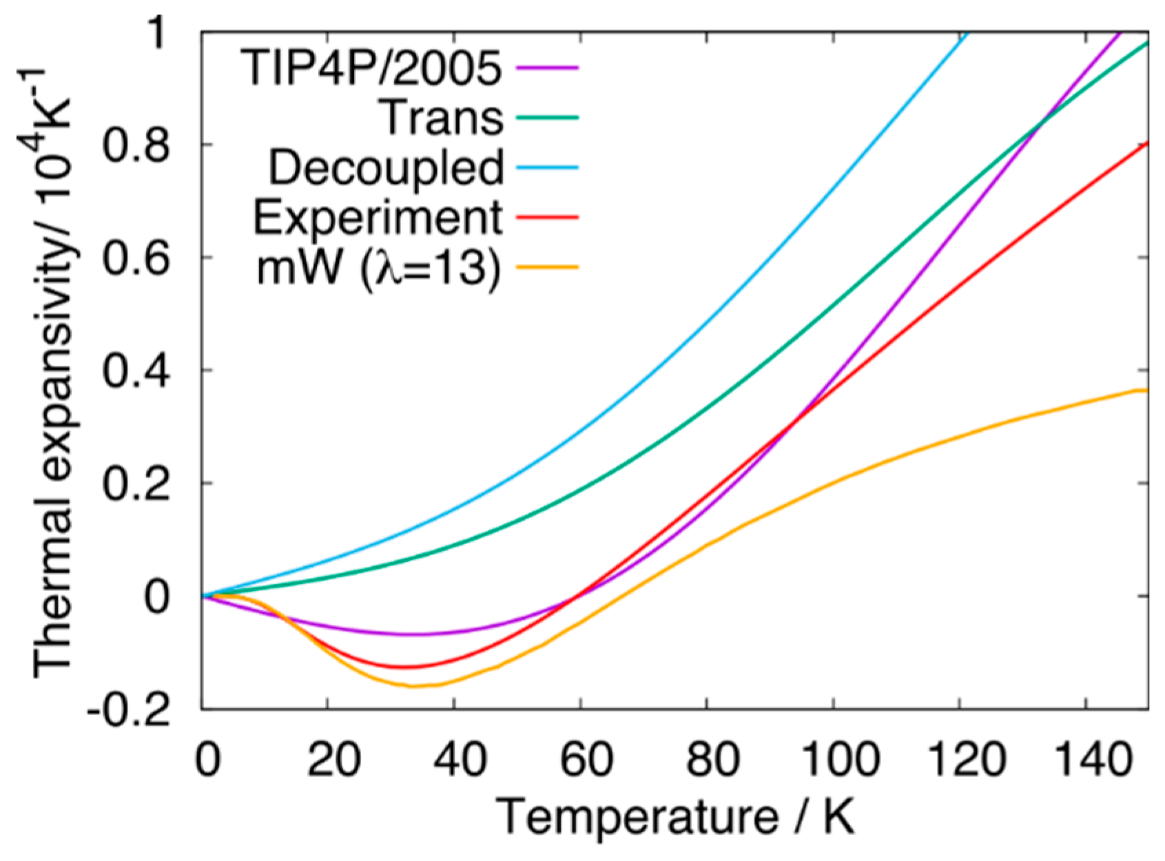
We calculate the temperature dependence of the molar volume for both the TIP4P/2005 model and the mW model. The purple curve in Figure 6 is the molar volume of ice Ic plotted against the temperature calculated with the all-atom TIP4P/2005 model. The value of 20.05 cm3 mol−1 is close to the experimental value for ice Ih, 19.3 cm3 mol−1 [3]. Figure 7 shows the thermal expansivity. The thermal expansivity of the TIP4P/2005 model is negative below 60 K, which is in agreement with the experimental result. We examine the effect of the coupling between the rotational and translational modes on the volume and its temperature dependence. The Hessian matrix, K, can be expressed as:
where t and r denote the translational and rotational components, respectively. We obtain a matrix Kb by removing the rotational-translational coupling elements, Ktr and Krt.
The thermodynamic properties without the rotational-translational coupling are calculated from the mode frequencies obtained by the diagonalization of the matrix Kb. Figure 6 shows that the volume of ice only slightly increases due to the removal of the coupling. However, the negative thermal expansivity disappears completely, as shown in Figure 7. It is also possible to eliminate the contributions from the rotational modes, as well as those from the rotational-translational coupling, by removing Krr in Equation (9). The volume calculated only from the translational motion is 19.38 3 cm3 mol−1, much smaller than the original value of the TIP4P/2005 model, 20.05 cm3 mol−1. Notwithstanding this, both the mW model and the TIP4P family reproduce the volume of liquid water fairly well [16], although there is a large discrepancy in the volume of ice I. The underestimation of the volume for the mW model may originate from the absence of the rotational modes. The shift to a higher frequency side upon compression in the TIP4P/2005 model is observed for the modes associated with the rotational motions, which is not shown but is a normal behavior against pressurization. This causes a decrease in the volume.
The thermal expansivity, α, can be expressed as:
where γ is the Grüneisen parameter, is the heat capacity, and is the isothermal compressibility. The Grüneisen parameter is expressed as:
where γi and are the Grüneisen parameter and heat capacity for the i-th mode, respectively. The mode Grüneisen parameter of the i-th mode is defined as:
The heat capacity of a mode is given by:
Figure 8 shows the frequency dependence of the heat capacities of the vibrational modes defined as:
for the mW model with λ = 13 at three different temperatures. The heat capacity is almost zero for modes with frequencies higher than 80 cm−1 at T = 20 K, reflecting the fact that only very low-frequency modes can be thermally excited at such a low temperature.
The mode Grüneisen parameter is calculated as follows. First, the mass-weighted Hessian matrix at the equilibrium volume, K0, is diagonalized as:
where Λ0 is the diagonalized matrix and U0 is the unitary matrix that diagonalizes K0. Next, the volume of the system is scaled isotropically by a factor of 1.0015, and the mass-weighted Hessian for the expanded system, Ke, is calculated. Similarly, the original system is scaled by 0.9985, and the mass-weighted Hessian for the shrunken system, Ks, is calculated. The mode frequencies of the expanded and the shrunken systems are calculated with the unitary matrix for the original volume:
and
The differential value, γi, is numerically calculated from Λe and Λs. Figure 9 shows the frequency dependence of the product γiCi for the mW model with λ = 13. The γi value is negative for the O-O-O bending modes around 50 cm−1. When the temperature is low enough, only this part contributes to the γ defined in Equation (11). At higher temperatures, the positive contributions from the high frequency O-O stretching modes become dominant because of the increase in Ci. Therefore, the negative thermal expansivity is observed only at low temperatures. A similar result was reported for the TIP4P model [6].
As shown in Figure 5, the negative thermal expansivity is found for the mW model when the λ parameter is small enough. Figure 10 presents the frequency dependence of γi. The mode Grüneisen parameters are positive even in the region around 50 cm−1 for the original λ value of 23.15. This is probably because the modes around 50 cm−1 with the original λ value have a lower O-O-O bending character. However, a decrease in the λ value can loosen the geometrical restriction of the arrangement on the three neighboring molecules and give rise to rather lower frequency modes, which may have the bending character.
5. Conclusions
We have calculated the chemical potential and volumetric properties of ice polymorphs with the original mW potential, applying the quasi-harmonic approximation. It is found that only several low-pressure ices (Ih, Ic, II, and III) are stable or metastable with the original mW model. The original mW model does not reproduce the negative thermal expansivity at low temperatures for ice I. A revision is proposed so as to recover the negative thermal expansivity. It is achieved by reducing one of the parameters of the force field model, λ, which was introduced for three molecules to favor the angle of the ideal tetrahedral arrangement, 109.47°. The origin of the negative thermal expansivity is examined for the revised mW model in terms of the anomalous mode Grüneisen parameters. In particular, the dependence of the mode Grüneisen parameters on the λ value is closely scrutinized. The magnitude of the negative mode Grüneisen parameters generally increases with decreasing λ value.
The calculated thermodynamic properties for mW ice are compared with those of a more realistic model, TIP4P/2005. The origin of the difference in the thermal expansivity is investigated by the chemical potential, whose vibrational free energy part is calculated from the block diagonal matrix in which all off-diagonal elements associated with translational-rotational degrees of freedom are removed. This decoupling of the translational and rotational motions eliminates the anomaly in the thermal expansivity and seems to be related to the observation that the negative thermal expansivity is not recovered with the original mW potential. The rotational degree of freedom may help to absorb the bare collisional motion between two adjacent oxygens through tight hydrogen bonding. The decrease in the λ value in mW, which loosens the geometrical restriction of the arrangement on the three neighboring molecules, seems to have a similar effect.
Author Contributions
M.M.H. performed the simulations and calculations, prepared the data, and wrote the paper; T.Y. co-wrote the paper; M.M. prepared the ice structures and revised the paper; H.T. conducted the project, wrote the programs for normal mode analysis, co-wrote and revised the paper.
Funding
This research was funded by JSPS KAKENHI grant number 17K19106 and MEXT as “Priority Issue on Post-Kcomputer” (Development of new fundamental technologies for high-efficiency energy creation, conversion/storage and use).
Conflicts of Interest
The authors declare no conflict of interest.
References
- Dantl, G. Wärmeausdehnung von H2O- und D2O-Einkristallen. Zeitschrift für Physik 1962, 166, 115–118. [Google Scholar] [CrossRef]
- Röttger, K.; Endriss, A.; Ihringer, J.; Doyle, S.; Kuhs, W.F. Lattice constants and thermal expansion of H2O and D2O ice Ih between 10 and 265 K. Addendum. Acta Crystallogr. B 2012, 68, 91. [Google Scholar] [CrossRef]
- Fortes, A.D. Accurate and precise lattice parameters of H2O and D2O ice Ih between 1.6 and 270 K from high-resolution time-of-flight neutron powder diffraction data. Acta Cryst. 2018, B74, 196–216. [Google Scholar]
- Buckingham, D.T.W.; Neumeier, J.J.; Masunaga, S.H.; Yu, Y.K. Thermal Expansion of Single-Crystal H2O and D2O Ice Ih. Phys. Rev. Lett. 2018, 121, 185505. [Google Scholar] [CrossRef]
- Fortes, A.D. Structural manifestation of partial proton ordering and defect mobility in ice Ih. Phys. Chem. Chem. Phys. 2019, 21, 8264–8474. [Google Scholar] [CrossRef]
- Tanaka, H. Thermodynamic stability and negative thermal expansion of hexagonal and cubic ices. J. Chem. Phys. 1998, 108, 4887–4893. [Google Scholar] [CrossRef]
- Grüneisen, E. Theorie des festen Zustandes einatomiger Elemente. Annalen der Physik 1912, 344, 257–306. [Google Scholar] [CrossRef]
- Nakamura, T.; Matsumoto, M.; Yagasaki, T.; Tanaka, H. Thermodynamic Stability of Ice II and Its Hydrogen-Disordered Counterpart: Role of Zero-Point Energy. J. Phys. Chem. B 2016, 120, 1843–1848. [Google Scholar] [CrossRef]
- Petrenko, V.F.; Whitworth, R.W. Physics of Ice; Oxford University Press: Oxford, UK, 1999. [Google Scholar]
- Grimme, S. Semiempirical GGA-type density functional constructed with a long-range dispersion correction. J. Comput. Chem. 2006, 27, 1787–1799. [Google Scholar] [CrossRef]
- Pamuk, B.; Soler, J.M.; Ramìrez, R.; Herrero, C.P.; Stephens, P.W.; Allen, P.B.; Fernàndez-Serra, M.-V. Anomalous Nuclear Quantum Effects in Ice. Phys. Rev. Lett. 2012, 108, 193003. [Google Scholar] [CrossRef] [PubMed]
- Salim, M.A.; Willow, S.Y.; Hirata, S. Ice Ih anomalies: Thermal contraction, anomalous volume isotope effect, and pressure-induced amorphization. J. Chem. Phys. 2016, 144, 204503. [Google Scholar] [CrossRef] [Green Version]
- Gupta, M.K.; Mittal, R.; Singh, B.; Mishra, S.K.; Adroja, D.T.; Fortes, A.D.; Chaplot, S.L. Phonons and anomalous thermal expansion behavior of H2O and D2O ice Ih. Phys. Rev. B 2018, 98, 104301. [Google Scholar] [CrossRef]
- McKinley, J.L.; Beran, G.J.O. Identifying pragmatic quasi-harmonic electronic structure approaches for modeling molecular crystal thermal expansion. Faraday Discuss. 2018, 211, 181–207. [Google Scholar] [CrossRef]
- Abascal, J.L.F.; Vega, C. A general purpose model for the condensed phases of water: TIP4P/2005. J. Chem. Phys. 2005, 123, 234505. [Google Scholar] [CrossRef]
- Sanz, E.; Vega, C.; Abascal, J.L.F.; MacDowell, L.G. Phase Diagram of Water from Computer Simulation. Phys. Rev. Lett. 2004, 92, 255701. [Google Scholar] [CrossRef] [PubMed]
- Aragones, J.L.; Vega, C. Plastic crystal phases of simple water models. J. Chem. Phys. 2009, 130, 244504. [Google Scholar] [CrossRef] [PubMed]
- Hirata, M.; Yagasaki, T.; Matsumoto, M.; Tanaka, H. Phase Diagram of TIP4P/2005 Water at High Pressure. Langmuir 2017, 33, 11561–11569. [Google Scholar] [CrossRef] [PubMed]
- Yagasaki, T.; Matsumoto, M.; Tanaka, H. Phase Diagrams of TIP4P/2005, SPC/E, and TIP5P Water at High Pressure. J. Phys. Chem. B 2018, 122, 7718–7725. [Google Scholar] [CrossRef] [PubMed]
- Jorgensen, W.L.; Chandrasekhar, J.; Madura, J.D.; Impey, R.W.; Klein, M.L. Comparison of simple potential functions for simulating liquid water. J. Chem. Phys. 1983, 79, 926–935. [Google Scholar] [CrossRef]
- Ramírez, R.; Neuerburg, N.; Fernández-Serra, M.-V.; Herrero, C.P. Quasi-harmonic approximation of thermodynamic properties of ice Ih, II, and III. J. Chem. Phys. 2012, 137, 044502–044513. [Google Scholar] [CrossRef]
- Molinero, V.; Moore, E.B. Water modeled as an intermediate element between carbon and silicon. J. Phys. Chem. B 2009, 113, 4008–4016. [Google Scholar] [CrossRef]
- Jacobson, L.C.; Hujo, W.; Molinero, V. Nucleation pathways of clathrate hydrates: Effect of guest size and solubility. J. Phys. Chem. B 2010, 114, 13796–13807. [Google Scholar] [CrossRef]
- Moore, E.B.; Molinero, V. Ice crystallization in water’s “no-man’s land”. J. Chem. Phys. 2010, 132, 244504. [Google Scholar] [CrossRef]
- Stillinger, F.H.; Weber, T.A. Computer simulation of local order in condensed phases of silicon. Phys. Rev. B 1985, 31, 5262–5271. [Google Scholar] [CrossRef]
- Laradji, M.; Landau, D.P.; Dünweg, B. Structural properties of Si1-xGex alloys: A Monte Carlo simulation with the Stillinger-Weber potential. Phys. Rev. B Condens. Matter 1995, 51, 4894–4902. [Google Scholar] [CrossRef]
- Takenaka, K. Negative thermal expansion materials: Technological key for control of thermal expansion. Sci. Technol. Adv. Mater. 2012, 13, 013001. [Google Scholar] [CrossRef]
- Fabian, J.; Allen, P.B. Thermal expansion and Grüneisen parameters of amorphous silicon: A realistic model calculation. Phys. Rev. Lett. 1997, 79, 1885. [Google Scholar] [CrossRef]
- Moore, E.B.; Molinero, V. Structural transformation in supercooled water controls the crystallization rate of ice. Nature 2011, 479, 506–508. [Google Scholar] [CrossRef]
- Matsumoto, M.; Yagasaki, T.; Tanaka, H. GenIce: Hydrogen-Disordered Ice Generator. J. Comput. Chem. 2018, 39, 61–64. [Google Scholar] [CrossRef]
- Li, J. Inelastic neutron scattering studies of hydrogen bonding in ices. J. Chem. Phys. 1996, 105, 6733–6755. [Google Scholar] [CrossRef]
Figure 1.
Densities of state of ice Ic calculated with the mW model (λ = 23.15) and that of the all-atom model. The experimental neutron scattering data for ice Ih is also shown [31].
Figure 1.
Densities of state of ice Ic calculated with the mW model (λ = 23.15) and that of the all-atom model. The experimental neutron scattering data for ice Ih is also shown [31].

Figure 2.
Thermodynamics potential, A + pV, for several ice structures at T = 20 K, obtained with the mW model. The curve for ice Ic overlaps completely with that of ice Ih.
Figure 2.
Thermodynamics potential, A + pV, for several ice structures at T = 20 K, obtained with the mW model. The curve for ice Ic overlaps completely with that of ice Ih.

Figure 3.
Molar volume of ice Ic as a function of temperature for the mW model, calculated with several λ values. The molar volume of ice Ih from the experimental data is also shown (red, right axis) [3].
Figure 3.
Molar volume of ice Ic as a function of temperature for the mW model, calculated with several λ values. The molar volume of ice Ih from the experimental data is also shown (red, right axis) [3].

Figure 4.
DOSs for ice Ic of the mW model with the original and modified λ values.

Figure 5.
Thermal expansivities of ice Ic calculated using the mW model with λ = 23.15 (purple line), 18.00 (green line), 15.00 (cyan line), and 13.00 (yellow line).
Figure 5.
Thermal expansivities of ice Ic calculated using the mW model with λ = 23.15 (purple line), 18.00 (green line), 15.00 (cyan line), and 13.00 (yellow line).

Figure 6.
Molar volume of ice Ic plotted against the temperature for the TIP4P/2005 model (purple), that calculated without the rotational-translational coupling (cyan), and that calculated only with the translational modes (green). The red curve is the volume of ice Ih from the experimental data. The volume of the mW model with λ = 13 is also shown (yellow, right axis).

Figure 7.
Thermal expansivity of ice Ic plotted against the temperature for the TIP4P/2005 model (purple), that calculated without the rotational-translational coupling (cyan), and that calculated only with the translational modes (green). The red curve is the thermal expansivity from the experimental data [3]. The thermal expansivity of the mW model with λ = 13 is also shown (yellow).

Figure 8.
Frequency dependence of the heat capacity of modes at temperatures 20 K (blue circle), 100 K (green diamond), and 400 K (red open square) for the mW model with λ = 13.
Figure 8.
Frequency dependence of the heat capacity of modes at temperatures 20 K (blue circle), 100 K (green diamond), and 400 K (red open square) for the mW model with λ = 13.

Figure 9.
Frequency dependence of γiCi at temperatures 20 K (blue circle), 100 K (green diamond), and 400 K (red open square) for the mW model with λ = 13.
Figure 9.
Frequency dependence of γiCi at temperatures 20 K (blue circle), 100 K (green diamond), and 400 K (red open square) for the mW model with λ = 13.

Figure 10.
Frequency dependence of the mode Grüneisen parameter for the original λ (blue circle), λ = 15 (green diamond), and λ = 13 (red open square).
Figure 10.
Frequency dependence of the mode Grüneisen parameter for the original λ (blue circle), λ = 15 (green diamond), and λ = 13 (red open square).


Table 1.
Parameters of the mW model [22].
Table 1.
Parameters of the mW model [22].
| A | 7.049556277 |
| B | 0.6022245584 |
| γ | 1.2 |
| a | 1.8 |
| λ | 23.15 |
| θ0 | 109.47° |
| σ | 0.23925 nm |
| ε | 25.895 kJ mol−1 |
© 2019 by the authors. Licensee MDPI, Basel, Switzerland. This article is an open access article distributed under the terms and conditions of the Creative Commons Attribution (CC BY) license (http://creativecommons.org/licenses/by/4.0/).
Share and Cite
MDPI and ACS Style
Huda, M.M.; Yagasaki, T.; Matsumoto, M.; Tanaka, H. Negative Thermal Expansivity of Ice: Comparison of the Monatomic mW Model with the All-Atom TIP4P/2005 Water Model. Crystals 2019, 9, 248. https://doi.org/10.3390/cryst9050248
AMA Style
Huda MM, Yagasaki T, Matsumoto M, Tanaka H. Negative Thermal Expansivity of Ice: Comparison of the Monatomic mW Model with the All-Atom TIP4P/2005 Water Model. Crystals. 2019; 9(5):248. https://doi.org/10.3390/cryst9050248
Chicago/Turabian StyleHuda, Muhammad Mahfuzh, Takuma Yagasaki, Masakazu Matsumoto, and Hideki Tanaka. 2019. "Negative Thermal Expansivity of Ice: Comparison of the Monatomic mW Model with the All-Atom TIP4P/2005 Water Model" Crystals 9, no. 5: 248. https://doi.org/10.3390/cryst9050248
Note that from the first issue of 2016, this journal uses article numbers instead of page numbers. See further details here.