On the Applicability of Stereological Methods for the Modelling of a Local Plastic Deformation in Grained Structure: Mathematical Principles

Abstract

Analysis of systems and structures from their cross-sectional images finds applications in many branches. Therefore, the question of content, quantity, and accuracy of information obtained from various techniques based on cross-sectional views of structures is particularly important. Application of conventional techniques for two-dimensional imaging on the analysis of structure from a cross-sectional image is limited. The reason for this limitation is the fact that these techniques use a fixed cross-sectional plane and therefore cannot check the 3D structural changes caused by deformation. Geometric orientation of a grained structure must be considered when data, scanned from a cross section, is processed in order to obtain information about local deformation in this structure. The so-called degree of structure orientation in 3D can be estimated experimentally from the cross-sectional image of the structure by the statistical (Saltykov) method of oriented testing lines. Subsequently if the correlation between orientation and deformation were to be known a detailed map of local deformation in the structure could be revealed. Unfortunately, exact theoretical works dealing with the assessment of local deformation by means of change of structure orientation in 3D are still missing. Our work seeks to partially remove this shortcoming. In our work we are interested in how the transformation of the image of a grained structure in a cross-sectional plane reflects structure deformation. An initial shape of grains is assumed which is transformed into a deformed shape by analytic calculation. We present brief mathematical derivations aimed at the problem of single grain-surface area deformation. The main goal of this work led to the design of a computationally low consuming procedure for quantification of local deformation in a grained structure based on the distortion of the image of this structure in a cross-sectional view.

1. Introduction

Final properties of components and systems prepared by means of forming technology are affected by mechanical working of the material. Essentially the forming process is a general method based on the deformation effects of external forces. These effects are macroscopic and do not reflect microscopic changes in the structure of material in all their diversity. The macroscopic strain cannot reflect all microstructural changes in the volume of deformed areas of the structure mainly in the case if only the surface layers of the material are deformed. To obtain exact information about changes in microstructure of materials in the whole volume of the bulk sample it is necessary to use suitable methods. Methods based on acoustic wave emission, analysis of dislocation, microhardness measurement, slip band observation, micromeshes method or macroscopic screw method can be used for this purpose and they are well developed. However, none of the mentioned available methods give analytical formulas relating local values of structure parameters and strain in any position of structure. The mentioned formulas are essential for a quantitative description of local changes induced by plastic deformation in the microstructure.

Grain boundary (interface between grains) is the main microstructural parameter in polycrystalline material. Grains have an isometric dimension when the grained structure is isotropic. The mean size of grains (grains size distribution) and the specific surface area of the grain boundaries are sufficient structural characteristics in this case. Grains have anisometric dimension when the grained structure is anisotropic and it is necessary to describe their orientation in space in this case.

In this context the question is how the spatial orientation of the grains themselves can be defined generally and exactly. It is possible to suspect intuitively that grain surface orientation in this sense can be evaluated by the prevailing orientation of the grain surface area elements. The next question is how can local deformation be estimated from the mentioned orientation of the grain surface.

Experimental observation and quantitative evaluation of shape and orientation of grains, domains or cells in grained, foam and cellular structures have been at the centre of attention of several authors already for some time [1,2]. Experimental observation has shown that the process of deformation is closely associated with the character of the crystallographic structure. Analysis of experimental data reveals that the grain boundaries and grain interactions during deformation play an important role in the process of deformation [3,4,5,6]. Various experimental procedures to characterize size, deformation, orientation, and position of single grain within the polycrystalline structure have been developed [7,8,9,10,11]. Most of these methods are already considered to be standard experimental techniques.

Calculation of grain boundary distortion during plastic straining has proven to be important in the theory of crystal plasticity and stereology [12,13,14,15,16]. Modelling of single crystal plasticity by numerical methods allows discussion of deviations of experimental results from ideal crystal behavior [17,18,19]. Information about the change of the grain surface area per unit volume as a function of deformation parameters is important in the production of steels [20].The amount of grain surface and grain edge per unit volume are parameters important in kinetic theory since both of them are heterogeneous nucleation sites. Recently published works demonstrate that problems of geometrical orientation of structure and distortion of structural units induced by deformation play an important role in different areas. We can mention for example biology where it is essential to clarify the organlevel tissue deformation dynamics to understand the morphogenetic mechanisms of organ development and regeneration. Construction and geometrical analyses of quantitative whole-organ tissue deformation maps must be realized for the evaluation of major morphogen and anisotropic tissue deformation along an axis [21].

2. Motivation and Aims

In recent years modern techniques and methods to observe crystal structure orientation have become available. For example, the image correlation method [22,23] is widely applied now. There is also a precise technique based on the triple points of grain boundaries [24,25] which can be followed by an electron backscatter diffraction (EBSD) method [26]. However, these methods have significant limitations (difficult sample preparation, requirement of conductive coatings, stability of electron beam for best data acquisition, etc.). In addition, all these methods are based on 2D observations. 3D measurement can only be done by stereology and high-resolution computed tomography (CT with nanofocus) could also handle 3D image reconstruction [27,28,29]. Stereological techniques provide quantitative information about a three-dimensional material from data scanned from two- dimensional planar sections of the structure. These techniques and methods are widely used today especially in the investigation of the character of coarse-grained and foamed structures.

Previous work has shown that there are several ways to evaluate grain orientation experimentally. However, the most acceptable way is the estimation of anisotropy based on stereological principle enabling determination of the “degree of grain orientation”. An anisotropic microstructure consists of (planar or linearly) oriented components which can be easily evaluated using stereological methods. We believe that results of such evaluation (degree of grain orientation in the volume of the plastically deformed structure) can be converted to values of local parameters of deformation. Therefore, it is sufficient to determine the degree of grain orientation to obtain a value of local strain.

We focus on the mathematical treatment of grain surface-deformation in our work. The problem of a grain-surface distortion induced by plastic deformation has been solved. We start with mathematics of grain behavior during linear deformation while we search for a formula enabling calculation of grain surface area change caused by deformation of grain using deformation tensor. Next, we propose a quantity for evaluation of degree of grain surface area orientation with respect to a certain vector in 3D space and discuss the correlation of this quantity with deformation parameters. Our contribution finishes with a brief commentary on the suggested technique of quantitative analysis, and outlines some key areas where further study is recommended.

We emphasize that strictly geometric orientation of the grain in 3D space is discussed in our work. The crystal structure within the grain is not analyzed (even though the concept of grain orientation is usually related with crystallographic orientation). A quantity κ is defined to evaluate the degree of orientation of the grain surface in relation to any direction. The presented work is focused on finding a correlation between the change in the degree of geometrical orientation of a grain and the deformation experienced by it. The case of a grain subjected to plastic deformation is studied in detail. The obtained results were applied for the particular case of a randomly oriented grained structure.

We present only a mathematical model for describing the deformation of a fictional, simplified grained structure—no real material is specified, nor is the actual deformation process described. We contribute thereby to the theoretical works on this topic published in the past [30,31,32,33,34]. A purely theoretical approach is presented. However, it has been shown that the discussed deformation mechanism, i.e., elongation (or the shortening) of grains under applied load, exists in a real-world material [35,36].

Stereological Method Based on Oriented Testing Lines

Direction of grain boundary orientation is the same as the direction of deformation. If the deformation scheme is known, grain boundaries can be decomposed into isotropic, planar, and linear oriented components using stereology method oriented test lines according to Saltykov [1] on propeller oriented metallographic prepared cutting planes. Grain boundaries are surfaces in volume and relative surface area, the average surface area to unit volume is measured—the isotropic, planar, and linear oriented parts of relative surface area. Intersections of cutting plane and the grain boundary surfaces are lines in the cutting plane. The average number of intersections per unit length of oriented test lines with grain boundaries P_L in the cutting plain is measured.

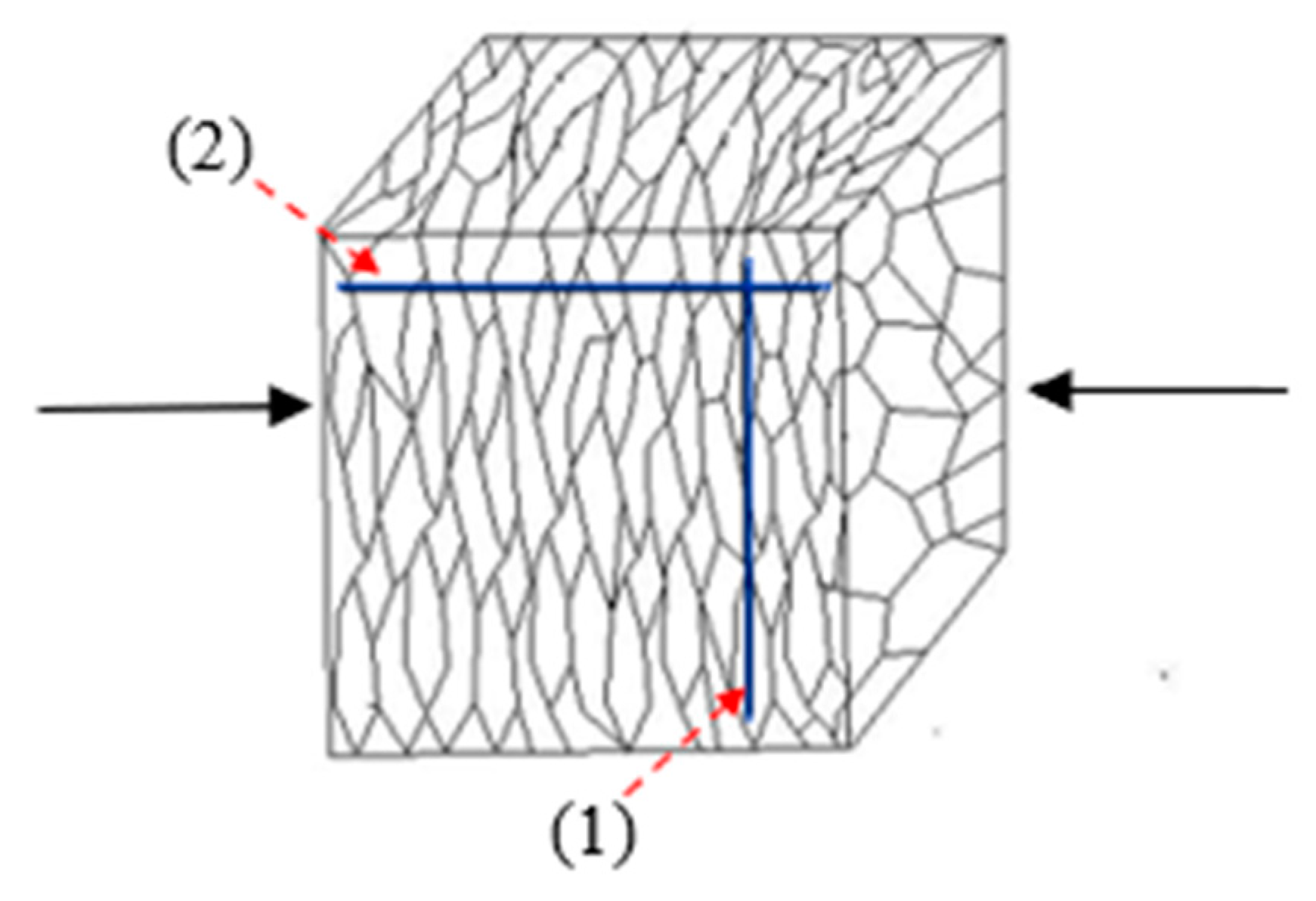
(a) Linear orientation of grain surface in sample volume

In the case of linear orientation of surfaces, the volume cutting plane, on which analysis is realized, must be parallel with the direction of orientation. In the perpendicular plane no orientation is observed. Test lines oriented parallel with the direction of orientation (1) intersect only the isotropic part of the surfaces in volume, test lines oriented perpendicular with direction of orientation (2) intersect isotropic and oriented part of surfaces in volume (see Figure 1). For the isotropic part of the relative surface area is as follows:

$${\left(S_V\right)}_{IS}=2{\left(P_L\right)}_P$$

(1)

where subscript IS means isotropic-randomly oriented and P means parallel orientation of test lines with direction of orientation. For the linear oriented part of the relative surface area it is as follows:

$${\left(S_V\right)}_{OR}=\frac{\pi }{2}\left[{\left(P_L\right)}_O-{\left(P_L\right)}_P\right]$$

(2)

where OR means oriented and subscript O perpendicular (orthogonal) orientation of test lines to direction of orientation. Total relative surface area is carried out by the sum of both parts:

$${\left(S_V\right)}_{TOT}=\frac{\pi }{2}{\left(P_L\right)}_O+\left(2-\frac{\pi }{2}\right){\left(P_L\right)}_P,$$

(3)

where subscript TOT means total.

(b) Planar orientation of grain surface in sample volume

In the case of planar orientation of surfaces in the volume cutting plane on which analysis is realized it must be perpendicular to the orientation plane. In the parallel plane no orientation is observed. Test lines oriented parallel to the plane of orientation (1) intersect only the isotropic part of the surfaces in volume, test lines oriented perpendicular to plane of orientation (2) intersect isotropic and oriented part of surfaces in volume (see Figure 2). For the isotropic part of the relative surface area it is as follows:

$${\left(S_V^{}\right)}_{IS}=2{\left(P_L\right)}_P$$

(4)

where subscript IS means isotropic-randomly oriented and P parallel orientation of test lines with plane of orientation. For the planar oriented part of the relative surface area it is as follows:

$${\left(S_V^{}\right)}_{OR}={\left(P_L\right)}_O-{\left(P_L\right)}_P$$

(5)

where OR means oriented and subscript O means perpendicular (orthogonal) orientation of test lines to the plane of orientation. Total relative surface area is carried out by the sum of both parts:

$${\left(S_V^{}\right)}_{TOT}={\left(P_L\right)}_O+{\left(P_L\right)}_P$$

(6)

where subscript TOT means total.

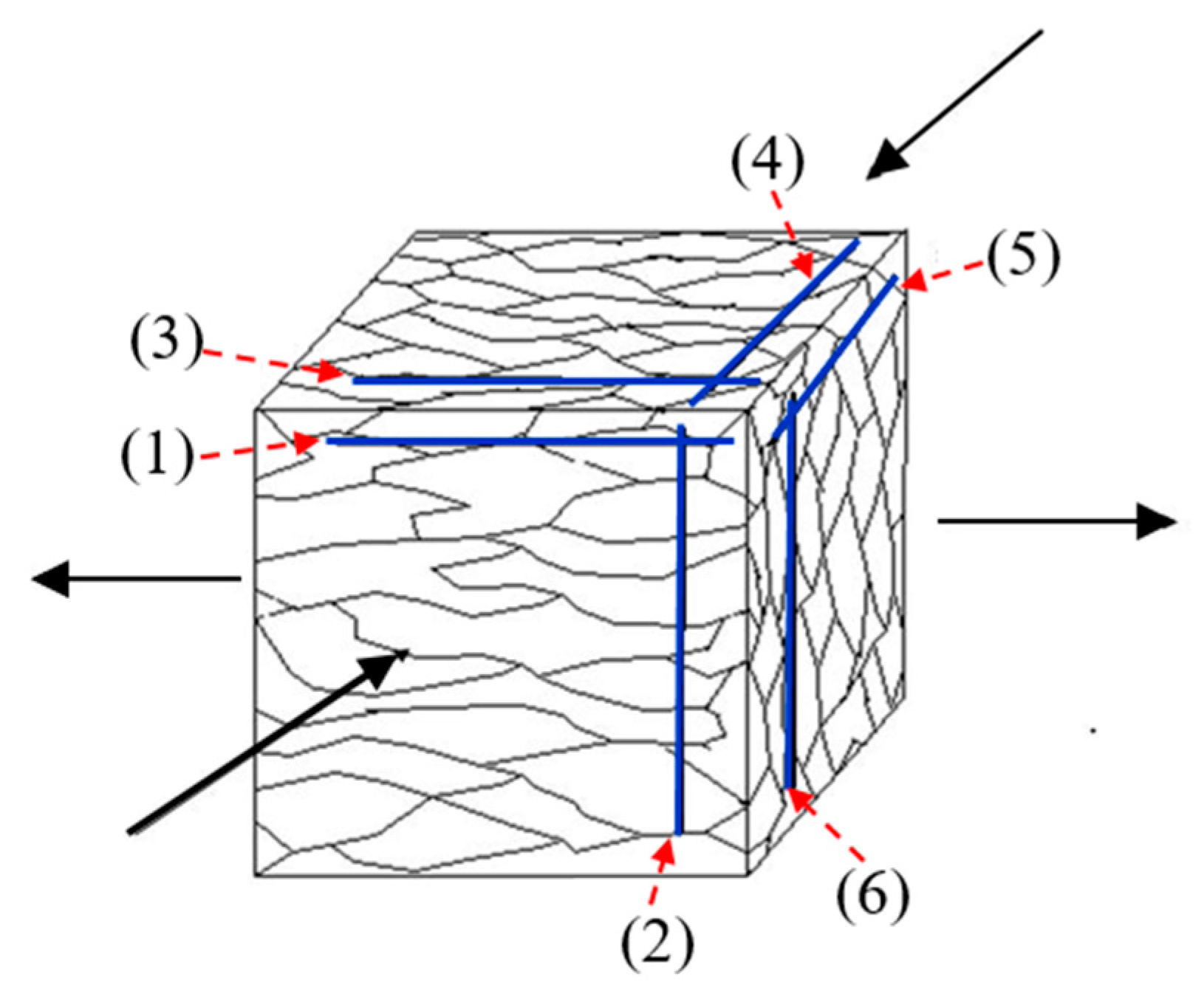
(c) Linear–planar orientation of grain surface in sample volume

In the case of linear–planar orientation of surfaces in volume the orientation is observed in all three orthogonal cutting planes, because the axis of linear orientation is perpendicular to the direction of the plane of orientation (direction of plane is normal to this)—see Figure 3. Each orientation component—planar and linear must be analyzed independently. Measurement must be realized on minimally two cutting planes. There are three possible cutting planes: cutting plane parallel with direction of linear orientation and parallel with plane of orientation, cutting plane perpendicular to direction of linear orientation and perpendicular to plane of orientation and cutting plane parallel with direction of linear orientation and perpendicular to plane of orientation.

The cutting plane parallel with the direction of linear orientation parallel with the plane of orientation test line, parallel with the direction of linear orientation (1) (see Figure 3) intersects only the isotropic part of the surfaces in volume (parameter (P_L)_PP), test lines oriented perpendicular with the direction of orientation (2) intersect the isotropic and linear oriented part of the surfaces in volume (parameter (P_L)_OP). For the isotropic and linear oriented part of the relative surface area it is:

$${\left(S_V^{}\right)}_{IS}=2{\left(P_L\right)}_{PP}$$

(7)

$${\left(S_V^{}\right)}_{ORL}=\frac{\pi }{2}\left[{\left(P_L\right)}_{OP}-{\left(P_L\right)}_{PP}\right]$$

(8)

where subscript ORL means linear oriented. The cutting plane perpendicular to the direction of linear orientation and perpendicular to the plane of the orientation test line parallel with the plane of orientation (6) intersects the isotropic and linear oriented parts of the surfaces in volume (parameter (P_L)_OP) (identical to test line 2), test lines oriented perpendicular to the plane of orientation (5) intersect the isotropic, linear and planar oriented parts of the surfaces in volume (parameter (P_L)_OO). For the planar oriented part of the relative surface area it is as follows:

$${\left(S_V^{}\right)}_{ORP}={\left(P_L\right)}_{OO}-{\left(P_L\right)}_{OP}$$

(9)

where subscript ORP means planar oriented.

On the cutting plane parallel with the direction of linear orientation and perpendicular to the plane of orientation test line parallel to the direction of linear orientation (the same as parallel to the plane orientation) (3) intersects only the isotropic part of the surfaces in volume (parameter (P_L)_PP) (identical to test line 1), the test line oriented perpendicular to the plane of orientation (4) intersects the isotropic, linear, and planar oriented parts of the surfaces in volume (parameter (P_L)_OO) (identical to test line 5). It is necessary for the determination of the quantitative parameters of the surfaces in volume with linear–planar orientation to use the system of three tested lines on two cutting planes and it is possible to form different combinations of tested lines (according to the identification in Figure 3)—(2 or 6) and (4 or 5) and (1 or 3).

(d) Experimental Quantification of degree of grain orientation

The degree of grain boundary orientation O can be estimated experimentally by means of formula:

$$O=\frac{{\left(S_V^{}\right)}_{OR}}{{\left(S_V^{}\right)}_{TOT}}$$

(10)

The degree of linear orientation surface (2D) in volume (3D) O_L of the linear orientated system of the surfaces in volume and degree of planar orientation O_P of planar orientated system of the surfaces in the volume are as follows:

$$O_L=1-2\left\{\frac{{\left(P_L\right)}_P}{\frac{\pi }{2}{\left(P_L\right)}_O+\left(2-\frac{\pi }{2}\right){\left(P_L\right)}_P}\right\}$$

(11)

$$O_P=1-2\left\{\frac{{\left(P_L\right)}_P}{{\left(P_L\right)}_O+{\left(P_L\right)}_P}\right\}$$

For the linear–planar oriented system of surfaces the degree of linear orientation O_LP, degree of planar orientation O_PL, and degree of total orientation O_TLP can be calculated by the following formulas:

$$\begin{gathered} O_{LP}=1-2\left\{\frac{2{\left(P_L\right)}_{PP}+{\left(P_L\right)}_{OO}-{\left(P_L\right)}_{OP}}{4{\left(P_L\right)}_{PP}+\pi \left[{\left(P_L\right)}_{OP}-\frac{\pi }{2}{\left(P_L\right)}_{PP}\right]+2\left[{\left(P_L\right)}_{OO}-{\left(P_L\right)}_{OP}\right]}\right\} \\ {O}_{PL}=1-2\left\{\frac{{\left(P_L\right)}_{PP}+\frac{\pi }{4}\left[{\left(P_L\right)}_{OP}-\frac{\pi }{2}{\left(P_L\right)}_{PP}\right]}{2{\left(P_L\right)}_{PP}+\frac{\pi }{2}\left[{\left(P_L\right)}_{OP}-\frac{\pi }{2}{\left(P_L\right)}_{PP}\right]+{\left(P_L\right)}_{OO}-{\left(P_L\right)}_{OP}}\right\} \\ {O}_{TLP}=1-2\left\{\frac{{\left(P_L\right)}_{PP}}{2{\left(P_L\right)}_{PP}+\frac{\pi }{2}\left[{\left(P_L\right)}_{OP}-\frac{\pi }{2}{\left(P_L\right)}_{PP}\right]+{\left(P_L\right)}_{OO}-{\left(P_L\right)}_{OP}}\right\} \end{gathered}$$

(12)

In the following text we deal with the theoretical analysis of the change of spatial orientation of grain during deformation and the possibilities of generalization of the mentioned relations (11) to (12).

3. Transformation of Grain-Surface Area at Linear Deformation

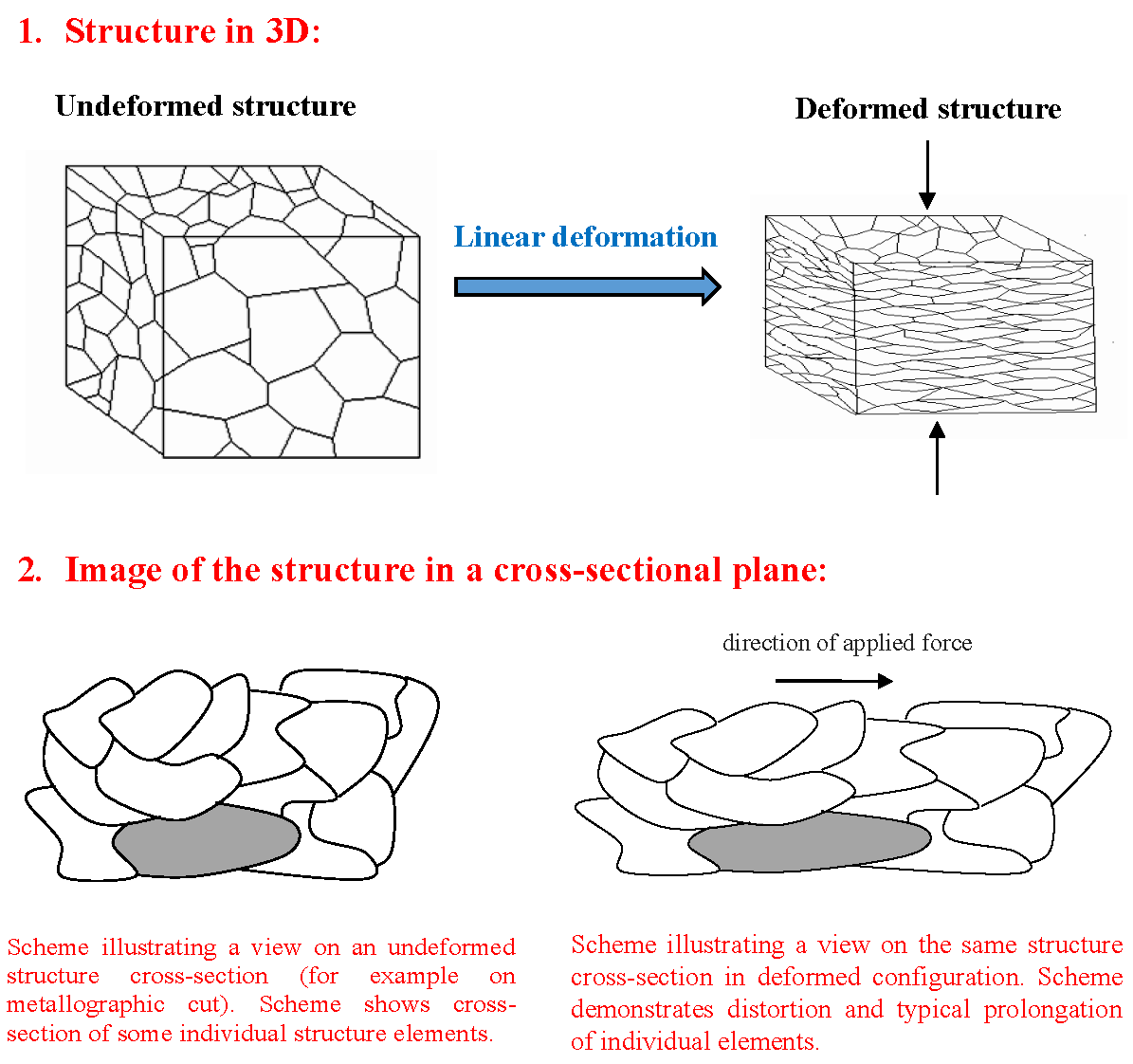
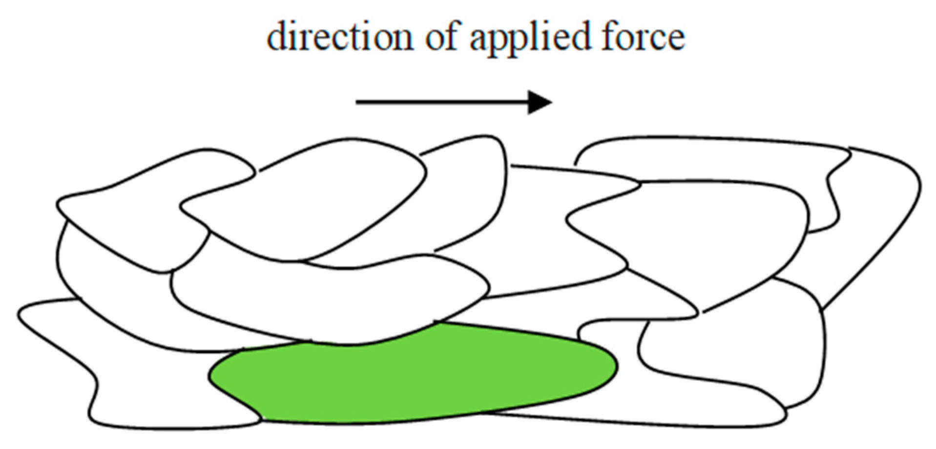
When a mechanical loading is applied most of the grains in a structure are submitted to a deformation. The deformation occurs according to the different orientations and influences from neighboring grains. If the grain is deformed a change in orientation and size of grain surface area are induced which leads to local heterogeneous plasticity. This is evident in the case where the typical grain prolongation in the direction of the loading force is visible (see Figure 4 and Figure 5).

This section provides an improved mathematical analysis of grain surface area transformation during linear grain deformation. Here we offer mathematical expressions usable in some models requiring the quantification of the deformed grain boundary surface. Relationships between coefficients of deformation tensor and change of grain surface are discussed. Results show how the specific area of the grain boundaries changes during local straining.

Let us discuss isotropic, linear elastic material with a grained structure. The parametrization of the surface of any single grain in 3D lies in the determination of the coordinates of each point on the surface:

$$X_i=X_i\left(u,v\right)$$

(13)

where i = 1, 2, 3 and u, v are parameters that changes in appropriate intervals. Then the position vectors of each point on the surface of the grain with any possible shape in undeformed configurations are as follows:

$$\overrightarrow{R}\left(u,v\right)=\left[X_1\left(u,v\right),X_2\left(u,v\right),X_3\left(u,v\right)\right],u\in \langle u_1,u_2\rangle v\in \langle v_1,v_2\rangle$$

(14)

Position vectors of each point on the surface of the same grain in the deformed state are as follows:

$$\overrightarrow{r}\left(u,v\right)=\left[x_1\left(u,v\right),x_2\left(u,v\right),x_3\left(u,v\right)\right],u\in \langle u_1^{\prime },u_2^{\prime }\rangle v\in \langle v_1^{\prime },v_2^{\prime }\rangle$$

(15)

In the general case, any 3D deformation can be described by a 3 × 3 deformation tensor:

$$\overrightarrow{\overrightarrow{\epsilon }}=\left(\begin{array}{ccc}{\epsilon }_{11}^{},& {\epsilon }_{12}^{},& {\epsilon }_{13}^{}\\ {\epsilon }_{21}^{},& {\epsilon }_{22}^{},& {\epsilon }_{23}^{}\\ {\epsilon }_{31}^{},& {\epsilon }_{32}^{},& {\epsilon }_{33}^{}\end{array}\right).$$

(16)

The deformation of grain for a small strain is linear. Therefore, using the notation mentioned above the deformation of the grain can be described by the following anisomorphic linear transformation:

$$\overrightarrow{r}=\overrightarrow{\overrightarrow{\epsilon }}\cdot \overrightarrow{R}\mathrm{or}{x}_i={\epsilon }_{ij}{X}_j$$

(17)

where i, j = 1, 2, 3 and ε_ij are coefficients of the deformation tensor (16). It is no problem to verify that ε_ij = δ_ij in the undeformed case (where δ_ij is the Kronecker symbol). We used the typical Einstein’s summation convention in the second formula in (17) whereby when an index variable appears twice in a single term it implies summation of that term over all the values of the index.

For simplicity this convention is used in all the following text.

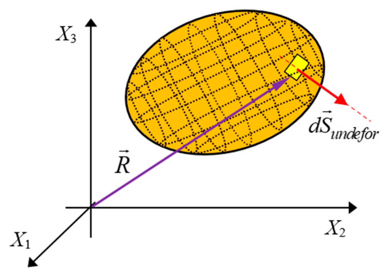
The surface element vectors for undeformed grain are determined as follows:

$$d^2{\overrightarrow{S}}_{undefor}=\left(\frac{\partial X_2}{\partial u}\frac{\partial X_3}{\partial v}-\frac{\partial X_3}{\partial u}\frac{\partial X_2}{\partial v}\right)\overrightarrow{i}-\left(\frac{\partial X_1}{\partial u}\frac{\partial X_3}{\partial v}-\frac{\partial X_3}{\partial u}\frac{\partial X_1}{\partial v}\right)\overrightarrow{j}+\left(\frac{\partial X_1}{\partial u}\frac{\partial X_2}{\partial v}-\frac{\partial X_2}{\partial u}\frac{\partial X_1}{\partial v}\right)\overrightarrow{k}$$

(18)

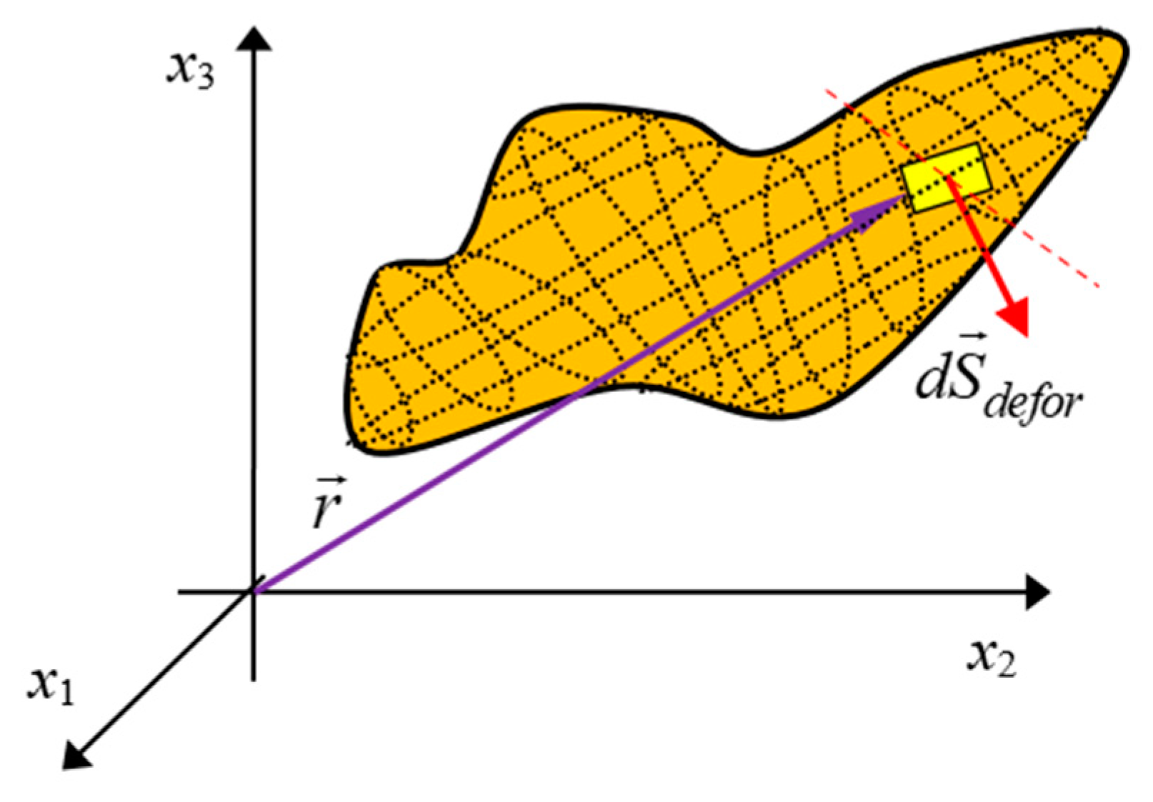
One of these vectors is shown in Figure 6. Using transformation (17) the vector of any surface element of the grain in the deformed state (see Figure 7) can be determined:

$$d^2{\overrightarrow{S}}_{defor}={\epsilon }_{2j}^{}{\epsilon }_{3k}^{}\left(\frac{\partial X_j}{\partial u}\frac{\partial X_k}{\partial v}-\frac{\partial X_j}{\partial v}\frac{\partial X_k}{\partial u}\right)\overrightarrow{i}-{\epsilon }_{1j}^{}{\epsilon }_{3k}^{}\left(\frac{\partial X_j}{\partial u}\frac{\partial X_k}{\partial v}-\frac{\partial X_j}{\partial v}\frac{\partial X_k}{\partial u}\right)\overrightarrow{j}+{\epsilon }_{1j}^{}{\epsilon }_{2k}^{}\left(\frac{\partial X_j}{\partial u}\frac{\partial X_k}{\partial v}-\frac{\partial X_j}{\partial v}\frac{\partial X_k}{\partial u}\right)\overrightarrow{k},$$

(19)

where i, j, k = 1, 2, 3.

After suitable re-indexing of the sums in Formula (19) the change of the mentioned vector of the surface element during deformation can be written as follows (please see details in Appendix A):

$$d^2{\overrightarrow{S}}_{defor}=\overrightarrow{\overrightarrow{\sigma }}\cdot d^2{\overrightarrow{S}}_{undefor}$$

(20)

where $\overrightarrow{\overrightarrow{\sigma }}$ can be introduced as a tensor of grain surface deformation. Coefficients of this tensor are related to the coefficients of the deformation tensor.

$${\sigma }_{wm}^{}={\left(-1\right)}^{w+m}det\left({\overrightarrow{\overrightarrow{\epsilon }}}_{mw}^{}\right)$$

(21)

where $det\left({\overrightarrow{\overrightarrow{\epsilon }}}_{mw}\right)$ is the subdeterminant of the matrix of the deformation tensor $\overrightarrow{\overrightarrow{\epsilon }}$. This subdeterminant is determined from the matrix of tensor $\overrightarrow{\overrightarrow{\epsilon }}$ by deleting the m-th row and w-th column. So, it is easily shows that coefficients of the tensor of grain surface deformation can be found as follows:

$${\sigma }_{wm}^{}={\epsilon }_{ik}^{}{\epsilon }_{jn}^{}-{\epsilon }_{in}^{}{\epsilon }_{jk}^{},$$

(22)

where indexes:

$$i=\frac{9-2w-{\left(-1\right)}^w}{4},j=\frac{15-2w+{\left(-1\right)}^w}{4}$$

(23)

$$k=\frac{12-2m-\left\{3+{\left(-1\right)}^m\right\}{\left(-1\right)}^{m+w}}{4},n=\frac{12-2m+\left\{3+{\left(-1\right)}^m\right\}{\left(-1\right)}^{m+w}}{4},w,m=1,2,3.$$

(24)

Then the size of the vector (20) of the deformed surface element is given as follows (please see details in Appendix B):

$${\left(d^2{S}_{defor}\right)}^2={\Gamma }_{jnks}\frac{\partial X_j}{\partial u}\frac{\partial X_n}{\partial u}\frac{\partial X_k}{\partial v}\frac{\partial X_s}{\partial v},$$

(25)

where coefficients:

$${\Gamma }_{jnks}={\displaystyle \sum _{\begin{array}{l}V\left(\left[p,q\right]\right),p\ne q\\ p,q\in \left\{1,2,3\right\}\end{array}}{\epsilon }_{pj}^{}{\epsilon }_{qk}^{}\left({\epsilon }_{pn}^{}{\epsilon }_{qs}^{}-{\epsilon }_{qn}^{}{\epsilon }_{ps}^{}\right)}$$

(26)

Notation under the summation symbol in (26) means the sum over all variations of indexes p, q while $p\ne q$. The entire surface area of the deformed grains can be determined by formula:

$$S_{defor}={\displaystyle \underset{v_1}{\overset{v_2}{\int }}{\displaystyle \underset{u_1}{\overset{u_2}{\int }}\sqrt{{\Gamma }_{jklm}\frac{\partial X_j}{\partial u}\frac{\partial X_k}{\partial v}\frac{\partial X_l}{\partial v}\frac{\partial X_m}{\partial u}}dudv}}.$$

(27)

where j, k, l, m = 1, 2, 3. We note, that we permanently use Einstein’s summation convention and the sum of 81 members is under the square root in Formula (27).

4. Quantitative Analysis of Grain Orientation: Projection Factor

In this section we define a novel scalar variable κ for quantification of the degree of grain- surface area orientation. First, there is briefly described motivation for such a way of introducing this variable. We believe that the variable κ helps to evaluate the grain orientation in a topological sense that is recognizably determined by the grain-surface area shape.

Orientations of surface elements of the grain in 3D are determined by the vectors $d\overrightarrow{S}$. These vectors are perpendicular to the grain-surface everywhere. Topologically the grain-surface area is considered to be a closed 2D manifold. Therefore the following holds:

$${\displaystyle \underset{\left(surface\right)}{\int }d\overrightarrow{S}}=\overrightarrow{0}$$

(28)

Grain boundaries are very important for energy balance of the grained structure. A special type of perturbance of this balance is induced by the loading force and for this reason a certain direction of orientation of the grain-surface elements becomes preferred under load. However, Formula (28) remains satisfied under load even in the unloaded condition. Atthe center of our attention is the question how could the correlation between the preferred orientation of the grain surface elements and the local structure deformation parameters be quantified.

Due to the planar character of the infinitesimal surface element dS there is no problem to define the orientation of this element in 3D just by means of the vector $d\overrightarrow{S}$. Then quantitative evaluation of the degree of orientation of this single surface element to the direction determined by the unit vector $\overrightarrow{\tau }$ can be performed using absolute value of scalar product:

$$\left|\overrightarrow{\tau }\cdot d\overrightarrow{S}\right|=dS\left|cos\left(\alpha \right)\right|=d{S}_p$$

(29)

where α is the angle between vectors $\overrightarrow{\tau }$ and $d\overrightarrow{S}$. The size of projection of the surface element dS_p to the plane perpendicular to the vector $\overrightarrow{\tau }$ is determined by quantity (29). Let S be the surface area of the whole grain. Then the quantity (29) calculated per unit surface area of the grain, i.e.:

$$\frac{dS\left|cos\left(\alpha \right)\right|}{S}$$

(30)

can determine a contribution of the element dS to the degree of whole grain-surface orientation to the direction determined by the unit vector $\overrightarrow{\tau }$. We need to introduce a variable κ enabling evaluation of the degree of whole grain-surface orientation to the direction determined by the unit vector $\overrightarrow{\tau }$ which would be also appropriate for quantitative analysis of grain surface distortion. The contribution rate of the surface element dS to the variable κ can be intuitively proposed by generalization of the quantity (31) as follows:

$$d\kappa =\frac{dS}{S}\xi \left(\alpha \right),$$

(31)

where ξ(α) is a value depending only on the angle α. Function ξ(α) must be designed in accordance with the requirement that the value κ corresponds to the quantities obtained from stereological measurements. In our work this function has been chosen in such a way that the limit of the values of variable κ correspond to values obtained in procedures realized on analysis of particle orientation using the Saltykov method (see Section 2 for an understanding of the principles). Consistent with this method we require:

$$\underset{\alpha \to \pi /2}{lim}\kappa =1,\underset{\alpha \to 0}{lim}\kappa =-1$$

(32)

So the following function can be used in this case:

$$\zeta \left(\alpha \right)=1-2\left|cos\left(\alpha \right)\right|$$

(33)

and contribution (31) can be written in the following form:

$$d\kappa =\left\{1-2\left|cos\left(\alpha \right)\right|\right\}\frac{dS}{S}=\frac{dS}{S}-2\frac{\left|\overrightarrow{\tau }\cdot d\overrightarrow{S}\right|}{S}.$$

(34)

Then the degree of whole grain-surface orientation to the direction determined by the unit vector $\overrightarrow{\tau }$ can be evaluated by the integration of (34) over the entire grain surface:

$$\kappa =1-2\frac{1}{S}{\displaystyle \underset{\left(Surface\right)}{\int }\left|\overrightarrow{\tau }\cdot d\overrightarrow{S}\right|}$$

(35)

In the following sections we examine how the quantity κ defined by (35) behaves during deformation and whether it allows analysis of the grain-surface area distortion induced by deformation. Namely if there is a vector $\overrightarrow{\gamma }$ satisfying:

$$\kappa \left(\overrightarrow{\gamma }\right)={\kappa }_{\max }$$

(36)

i.e., if the value of κ is maximal for vector $\overrightarrow{\gamma }$, this vector determines the preferred whole grain- surface area orientation (or grain orientation in a topological sense).

The degree of whole grain-surface orientation to the direction determined by the unit vector $\overrightarrow{\tau }$ in both deformed and undeformed configurations can be evaluated by Formula (35):

$${\kappa }_{undefor}=1-2\frac{{\displaystyle \underset{\left(Surface\right)}{\int }\left|\overrightarrow{\tau }\cdot d{\overrightarrow{S}}_{undefor}\right|}}{{\displaystyle \underset{\left(Surface\right)}{\int }\left|d{\overrightarrow{S}}_{undefor}\right|}},{\kappa }_{defor}=1-2\frac{{\displaystyle \underset{\left(surface\right)}{\int }\left|\overrightarrow{\tau }\cdot d{\overrightarrow{S}}_{defor}\right|}}{{\displaystyle \underset{\left(surface\right)}{\int }\left|d{\overrightarrow{S}}_{defor}\right|}}.$$

(37)

Let $\overrightarrow{\rho }$ be the unit vector parallel to the vector of the grain-surface element of undeformed grain, $d{\overrightarrow{S}}_{undefor}=\overrightarrow{\rho }d{S}_{undefor}$ i.e.,: where $\left|\overrightarrow{\rho }\right|=1$.

Taking into account the Formula (38) and considering the fact:

$$\overrightarrow{\tau }\cdot d^2{\overrightarrow{S}}_{defor}=\overrightarrow{\tau }\cdot \left(\overrightarrow{\overrightarrow{\sigma }}\cdot d^2{\overrightarrow{S}}_{undefor}\right)=\left({\overrightarrow{\overrightarrow{\sigma }}}^T\cdot \overrightarrow{\tau }\right)\cdot d^2{\overrightarrow{S}}_{undefor},$$

(38)

where ${\overrightarrow{\overrightarrow{\sigma }}}^T$ is the transposed tensor to the grain surface deformation tensor $\overrightarrow{\overrightarrow{\sigma }}$ determined by (22), Formulas (37) can be rewritten in the following form:

$${\kappa }_{undefor}=1-2\frac{{\displaystyle \underset{\left(Surface\right)}{\int }\left|\overrightarrow{\tau }\cdot d{\overrightarrow{S}}_{undefor}\right|}}{{\displaystyle \underset{\left(Surface\right)}{\int }\left|\overrightarrow{\rho }\right|d{S}_{undefor}}},{\kappa }_{defor}=1-2\frac{{\displaystyle \underset{\left(Surface\right)}{\int }\left|\left({\overrightarrow{\overrightarrow{\sigma }}}^T\cdot \overrightarrow{\tau }\right)\cdot d{\overrightarrow{S}}_{undefor}\right|}}{{\displaystyle \underset{\left(Surface\right)}{\int }\left|\overrightarrow{\overrightarrow{\sigma }}\cdot \overrightarrow{\rho }\right|d{S}_{undefor}}}$$

(39)

As can be concluded from comparison of the above Equation (39), transformation of the value κ during grain deformation can be realized as follows:

$$\overrightarrow{\tau }\to {\overrightarrow{\overrightarrow{\sigma }}}^T\cdot \overrightarrow{\tau }\wedge \overrightarrow{\rho }\to \overrightarrow{\overrightarrow{\sigma }}\cdot \overrightarrow{\rho }$$

(40)

Equation (39) correspond to Formulas (11) to (12). They can be considered as a generalized formula for the degree of grain orientation measured by the Saltykov method. As can be seen from (39) the transformation of κ during grain deformation is relatively complicated. We will not examine the properties of this transformation in detail. However, we want to point out the fact that that it is sufficient to integrate over the surface of the undeformed grain in both of the Formula (39). So, to determine the value κ in deformed configuration we need to know only the shape of the undeformed grain and the coefficients of the deformation tensor ε_ij. We believe, that κ is a scalar variable acceptable for the quantitative evaluation of grain-surface distortion during local deformation of the grained structure.

5. The Case of Plastic Deformation

The fundamental assumption used to establish the theory of plasticity is that plastic deformation is isochoric or volume preserving. Next, we apply the results obtained in previous sections to the case of plastic grain deformation, i.e., deformation in which the change of volume of grain is zero.

Conservation of grain volume during the plastic deformation process can be described by the formula:

V_undefor = V_defor

(41)

The Gauss formula can be used for determination of grain volume in both undeformed (V_undefor) and deformed (V_defor) configurations:

$${\displaystyle \underset{\left(S_{undefor}\right)}{\int }\overrightarrow{R}\cdot d{\overrightarrow{S}}_{undefor}}={\displaystyle \underset{\left(V_{undefor}\right)}{\int }div\left(\overrightarrow{R}\right)dV}=3V_{undefor},{\displaystyle \underset{\left(S_{defor}\right)}{\int }\overrightarrow{r}\cdot d{\overrightarrow{S}}_{defor}}={\displaystyle \underset{\left(V_{defor}\right)}{\int }div\left(\overrightarrow{r}\right)d{V}^{\prime }}=3V_{defor}.$$

(42)

A comparison of the Equation (42) shows:

$${\displaystyle \underset{\left(S_{undefor}\right)}{\int }\overrightarrow{R}\cdot d{\overrightarrow{S}}_{undefor}}={\displaystyle \underset{\left(S_{defor}\right)}{\int }\overrightarrow{r}\cdot d{\overrightarrow{S}}_{defor}}={\displaystyle \underset{\left(S_{undefor}\right)}{\int }\left\{{\overrightarrow{\overrightarrow{\sigma }}}^T\cdot \left(\overrightarrow{\overrightarrow{\epsilon }}\cdot \overrightarrow{R}\right)\right\}\cdot }d{\overrightarrow{S}}_{undefor}$$

(43)

where Formulas (17) and (20) were used. It is necessary to integrate over the same (but any) surface area on both sides of the previous Equation (43). Therefore, for plastic deformations the following applies:

$$\overrightarrow{R}={\overrightarrow{\overrightarrow{\sigma }}}^T\cdot \left(\overrightarrow{\overrightarrow{\epsilon }}\cdot \overrightarrow{R}\right),{\overrightarrow{\overrightarrow{\sigma }}}^T={\overrightarrow{\overrightarrow{\epsilon }}}^{-1}\mathrm{respectively}.$$

(44)

As follows from Formula (44) the transposed tensor of the grain surface deformation tensor is inverse to the deformation tensor in the case of plastic deformation. If we consider Formula (43), the following equation can be written in the case of plastic deformation (please see details in Appendix C):

$$\left\{\left({\epsilon }_{1n}{\epsilon }_{2j}{\epsilon }_{3k}-{\epsilon }_{2n}{\epsilon }_{1j}{\epsilon }_{3k}+{\epsilon }_{3n}{\epsilon }_{1j}{\epsilon }_{2k}\right)-\left({\delta }_{1n}{\delta }_{2j}{\delta }_{3k}-{\delta }_{2n}{\delta }_{1j}{\delta }_{3k}+{\delta }_{3n}{\delta }_{1j}{\delta }_{2k}\right)\right\}\left(\frac{\partial X_j}{\partial u}\frac{\partial X_k}{\partial v}-\frac{\partial X_j}{\partial v}\frac{\partial X_k}{\partial u}\right)X_n=0.$$

(45)

Equation (45) must be satisfied for any function $X_i=X_i\left(u,v\right)$ in the case of grain volume conservation during plastic deformation. If (45) is expanded without further assumptions, this leads to the following 27 equations:

$${\epsilon }_{1n}\left({\epsilon }_{2j}{\epsilon }_{3k}-{\epsilon }_{2k}{\epsilon }_{3j}\right)-{\epsilon }_{2n}\left({\epsilon }_{1j}{\epsilon }_{3k}-{\epsilon }_{1k}{\epsilon }_{3j}\right)+{\epsilon }_{3n}\left({\epsilon }_{1j}{\epsilon }_{2k}-{\epsilon }_{1k}{\epsilon }_{2j}\right)-$$

$$-{\delta }_{1n}\left({\delta }_{2j}{\delta }_{3k}-{\delta }_{2k}{\delta }_{3j}\right)+{\delta }_{2n}\left({\delta }_{1j}{\delta }_{3k}-{\delta }_{1k}{\delta }_{3j}\right)-{\delta }_{3n}\left({\delta }_{1j}{\delta }_{2k}-{\delta }_{1k}{\delta }_{2j}\right)=0\hspace{1em}\dots \forall \hspace{1em}n,j,k$$

(46)

i.e., the following equation must be satisfied in the case of plastic deformation (please see details in Appendix D):

$$det\left(\overrightarrow{\overrightarrow{\epsilon }}\right)=1$$

(47)

Next, the conditions for the deformation tensor can be considered in the case of plastic deformation of a homogeneous and isotropic grained structure:

$${\epsilon }_{ji}^{}=0\mathrm{for}\mathrm{all}i\ne j\ne k\hspace{1em}\wedge \hspace{1em}det\left(\overrightarrow{\overrightarrow{\epsilon }}\right)={\epsilon }_{ii}^{}{\epsilon }_{jj}^{}{\epsilon }_{kk}^{}=1.$$

(48)

Elements of the deformation tensor are directly related to grain prolongation (contraction) δ (−1 < δ < ∞) in this case. If the loading force is applied in the direction of the x-axis the following holds:

$${\epsilon }_{11}^{}=\delta +1,{\epsilon }_{22}^{}={\epsilon }_{33}^{}=\frac{1}{\sqrt{\delta +1}}$$

(49)

and due to Formula (44) the degree of grain surface area orientation (39) can be modified to the following form:

$${\kappa }_{defor}=1-2\frac{{\displaystyle \underset{\left(Surface\right)}{\int }\left|\left({\overrightarrow{\overrightarrow{\epsilon }}}^{-1}\cdot \overrightarrow{\tau }\right)\cdot d{\overrightarrow{S}}_{undefor}\right|}}{{\displaystyle \underset{\left(Surface\right)}{\int }\left|{\overrightarrow{\overrightarrow{\epsilon }}}^{-1}\cdot \overrightarrow{\rho }\right|d{S}_{undefor}}}9.$$

(50)

Detailed information about the shape of the grain is necessary for the practical application of the result (39) and (50) because integrals in these formulas are integrated over the entire surface of the grain. However, there is no possibility to determine the real shape of each grain in the material structure exactly. Therefore, deformation of the model of the grained structure is usually investigated. Models of the grained structure consist of grains with various idealized shapes. For instance, deformation of spheres can be considered since spheres are not space filling and have no edges. Deformation of cubes can be also investigated, and mathematical analysis can be simplified, but cubes are unfortunately clearly poor for approximations to the shapes of real grains. The tetrakaidecahedronal shape of the grain is very suitable for modeling because it is space filling and approximately identical with the shape of real grains observed metallographically in the undeformed state [37,38].

Models of grained structures based on the specific idealized shape of grains allow examination of the relationship between grain orientation and local deformation but the problem of non-zero grain orientation in the case of zero value of initial deformation of the structure often arises from such models [39,40].

Our method presented in the next section does not evaluate the orientation of one idealized grain placed in the structure but investigates the orientation of all grain boundaries localized in a certain area of the grained structure. Integrals in the Formulas (39) and (50) must be integrated over the surface of all grain boundaries in this area. The relationship between grain orientation in this local area and local deformation can be determined from these formulas in this case.

6. Random Matrix Approximation

In this section we explain the applicability of results presented above in the modelling of local deformations in grained structures. Integrals in (39) should be integrated over the entire surface of the grain boundaries when the degree of orientation of the whole grained structure κ is evaluated.

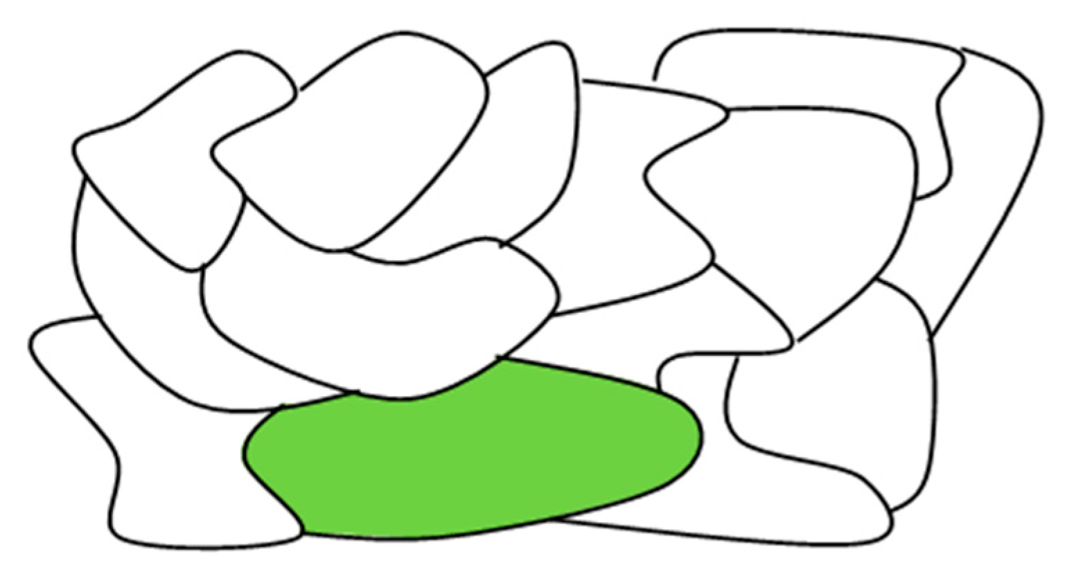
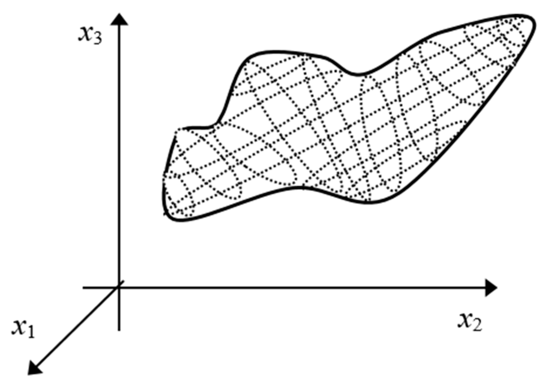
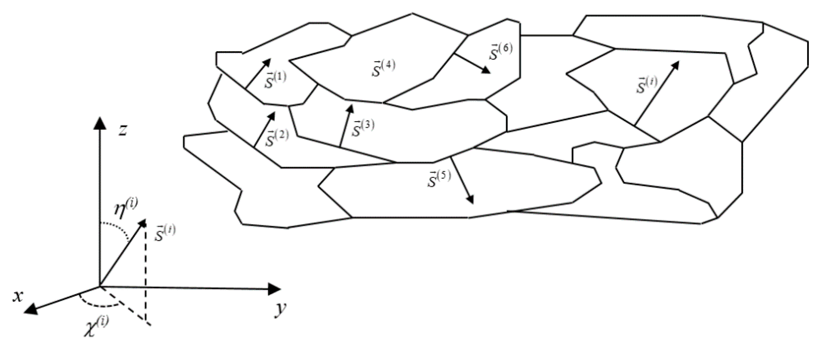
For computational purposes, integrals in the Formula (39) can be written in the form of summation over the infinitely small areas placed around the wholegrain boundary surface (see Figure 8 and Figure 9). A cross-sectional image of such a model of a granular structure is shown in Figure 10. So, we obtain the following:

$${\kappa }_{defor}\approx 1-2\frac{{\displaystyle \sum _{i=1}^N\left|\left({\overrightarrow{\overrightarrow{\sigma }}}^T\cdot \overrightarrow{\tau }\right)\cdot {\overrightarrow{S}}_{undefor}^{\left(i\right)}\right|}}{{\displaystyle \sum _{i=1}^N\left|\overrightarrow{\overrightarrow{\sigma }}\cdot {\overrightarrow{\rho }}^{\left(i\right)}\right|S_{}^{\left(i\right)}}}$$

(51)

where $\overrightarrow{\tau }=\left[{\tau }_1,{\tau }_2,{\tau }_3\right]$ is any unit vector (i.e., ${\tau }_1^2+{\tau }_2^2+{\tau }_3^2=1$) and ${\overrightarrow{\rho }}^{\left(i\right)}$ is unit vector perpendicular to the i-th grain-surface element of undeformed grain:

$${\overrightarrow{S}}_{undefor}^{\left(i\right)}={\overrightarrow{\rho }}^{\left(i\right)}{S}^{\left(i\right)}.$$

(52)

Vector ${\overrightarrow{\rho }}^{\left(i\right)}$ can be written in the form:

$${\overrightarrow{\rho }}^{\left(i\right)}=\left[sin\left({\eta }^{\left(i\right)}\right)cos\left({\chi }^{\left(i\right)}\right),sin\left({\eta }^{\left(i\right)}\right)sin\left({\chi }^{\left(i\right)}\right),cos\left({\eta }^{\left(i\right)}\right)\right]$$

while ${\eta }^{\left(i\right)}$ and ${\chi }^{\left(i\right)}$ are angles which determine the orientation of the i-th grain-surface element. Then the following applies:

$${\overrightarrow{S}}_{undefor}^{\left(i\right)}=\left[S_1^{\left(i\right)},S_2^{\left(i\right)},S_3^{\left(i\right)}\right]=\left[S_{}^{\left(i\right)}sin\left({\eta }^{\left(i\right)}\right)cos\left({\chi }^{\left(i\right)}\right),S_{}^{\left(i\right)}sin\left({\eta }^{\left(i\right)}\right)sin\left({\chi }^{\left(i\right)}\right),S_{}^{\left(i\right)}cos\left({\eta }^{\left(i\right)}\right)\right]$$

(53)

If we use result (22) and notation (53), the sums in the Formula (51) can be determined as (please see details in Appendix E):

$$\begin{array}{l}{\displaystyle \sum _{i=1}^N\left|\left({\overrightarrow{\overrightarrow{\sigma }}}^T\cdot \overrightarrow{\tau }\right)\cdot {\overrightarrow{\rho }}^{\left(i\right)}{S}^{\left(i\right)}\right|}=\\ \hspace{1em}={\displaystyle \sum _{i=1}^N|\{\left[\left({\epsilon }_{22}^{}{\epsilon }_{33}^{}-{\epsilon }_{23}^{}{\epsilon }_{32}^{}\right)sin\left({\eta }^{\left(i\right)}\right)cos\left({\chi }^{\left(i\right)}\right)+\left({\epsilon }_{23}^{}{\epsilon }_{31}^{}-{\epsilon }_{21}^{}{\epsilon }_{33}^{}\right)sin\left({\eta }^{\left(i\right)}\right)sin\left({\chi }^{\left(i\right)}\right)+\left({\epsilon }_{21}^{}{\epsilon }_{32}^{}-{\epsilon }_{22}^{}{\epsilon }_{31}^{}\right)cos\left({\eta }^{\left(i\right)}\right)\right]{\tau }_1+}\\ \hspace{1em}+\left[\left({\epsilon }_{13}^{}{\epsilon }_{32}^{}-{\epsilon }_{12}^{}{\epsilon }_{33}^{}\right)sin\left({\eta }^{\left(i\right)}\right)cos\left({\chi }^{\left(i\right)}\right)+\left({\epsilon }_{11}^{}{\epsilon }_{33}^{}-{\epsilon }_{13}^{}{\epsilon }_{31}^{}\right)sin\left({\eta }^{\left(i\right)}\right)sin\left({\chi }^{\left(i\right)}\right)+\left({\epsilon }_{12}^{}{\epsilon }_{31}^{}-{\epsilon }_{11}^{}{\epsilon }_{32}^{}\right)cos\left({\eta }^{\left(i\right)}\right)\right]{\tau }_2+\\ \hspace{1em}+\left[\left({\epsilon }_{12}^{}{\epsilon }_{23}^{}-{\epsilon }_{13}^{}{\epsilon }_{22}^{}\right)sin\left({\eta }^{\left(i\right)}\right)cos\left({\chi }^{\left(i\right)}\right)+\left({\epsilon }_{13}^{}{\epsilon }_{21}^{}-{\epsilon }_{11}^{}{\epsilon }_{23}^{}\right)sin\left({\eta }^{\left(i\right)}\right)sin\left({\chi }^{\left(i\right)}\right)+\left({\epsilon }_{11}^{}{\epsilon }_{22}^{}-{\epsilon }_{12}^{}{\epsilon }_{21}^{}\right)cos\left({\eta }^{\left(i\right)}\right)\right]{\tau }_3\}{S}^{\left(i\right)}|\end{array}$$

(54)

$$\begin{array}{c}{\displaystyle \sum _{i=1}^N\left|\overrightarrow{\overrightarrow{\sigma }}\cdot {\overrightarrow{\rho }}^{\left(i\right)}\right|S_{}^{\left(i\right)}}=\hfill \\ ={\displaystyle \sum _{i=1}^N[{\left\{\left({\epsilon }_{22}^{}{\epsilon }_{33}^{}-{\epsilon }_{23}^{}{\epsilon }_{32}^{}\right)cos\left({\chi }^{\left(i\right)}\right)sin\left({\eta }^{\left(i\right)}\right)-\left({\epsilon }_{21}^{}{\epsilon }_{33}^{}-{\epsilon }_{23}^{}{\epsilon }_{31}^{}\right)sin\left({\chi }^{\left(i\right)}\right)sin\left({\eta }^{\left(i\right)}\right)+\left({\epsilon }_{21}^{}{\epsilon }_{32}^{}-{\epsilon }_{22}^{}{\epsilon }_{31}^{}\right)cos\left({\eta }^{\left(i\right)}\right)\right\}}^2+}\hfill \\ +{\left\{\left({\epsilon }_{13}^{}{\epsilon }_{32}^{}-{\epsilon }_{12}^{}{\epsilon }_{33}^{}\right)cos\left({\chi }^{\left(i\right)}\right)sin\left({\eta }^{\left(i\right)}\right)-\left({\epsilon }_{13}^{}{\epsilon }_{31}^{}-{\epsilon }_{11}^{}{\epsilon }_{33}^{}\right)sin\left({\chi }^{\left(i\right)}\right)sin\left({\eta }^{\left(i\right)}\right)+\left({\epsilon }_{12}^{}{\epsilon }_{31}^{}-{\epsilon }_{11}^{}{\epsilon }_{32}^{}\right)cos\left({\eta }^{\left(i\right)}\right)\right\}}^2+\hfill \\ {+{\left\{\left({\epsilon }_{12}^{}{\epsilon }_{23}^{}-{\epsilon }_{13}^{}{\epsilon }_{22}^{}\right)cos\left({\chi }^{\left(i\right)}\right)sin\left({\eta }^{\left(i\right)}\right)-\left({\epsilon }_{11}^{}{\epsilon }_{23}^{}-{\epsilon }_{13}^{}{\epsilon }_{21}^{}\right)sin\left({\chi }^{\left(i\right)}\right)sin\left({\eta }^{\left(i\right)}\right)+\left({\epsilon }_{11}^{}{\epsilon }_{22}^{}-{\epsilon }_{12}^{}{\epsilon }_{21}^{}\right)cos\left({\eta }^{\left(i\right)}\right)\right\}}^2]}^{\frac{1}{2}}{S}^{\left(i\right)}\hfill \end{array}$$

(55)

The degree of whole grained structure orientation κ to the direction determined by the unit vector $\overrightarrow{\tau }$ was calculated by means of the Formula (51) while the sums in the numerator and denominator in the second member on the right side of this formula were determined by (54) and (55).

Any randomly oriented surface element on the grain boundary S⁽ⁱ⁾ in the given bulk grained structure can be considered in the calculation of κ if the corresponding parameters η⁽ⁱ⁾ and χ⁽ⁱ⁾ are applied. Therefore, random values of angles η⁽ⁱ⁾ and χ⁽ⁱ⁾ should be substituted step by step into Formulas (54) and (55) during the calculation progress. This procedure of determination of the parameter κ can be formulated using the following random matrices directly pertaining to the deformation tensor only:

$${\tilde{A}}_1^{\left(i\right)}=\left(\begin{array}{ccc}sin\left({\eta }^{\left(i\right)}\right)cos\left({\chi }^{\left(i\right)}\right),& sin\left({\eta }^{\left(i\right)}\right)sin\left({\chi }^{\left(i\right)}\right),& cos\left({\eta }^{\left(i\right)}\right)\\ {\epsilon }_{21}^{},& {\epsilon }_{22}^{},& {\epsilon }_{23}^{}\\ {\epsilon }_{31}^{},& {\epsilon }_{32}^{},& {\epsilon }_{33}^{}\end{array}\right)$$

(56)

$${\tilde{A}}_2^{\left(i\right)}=\left(\begin{array}{ccc}{\epsilon }_{11}^{},& {\epsilon }_{12}^{},& {\epsilon }_{13}^{}\\ sin\left({\eta }^{\left(i\right)}\right)cos\left({\chi }^{\left(i\right)}\right),& sin\left({\eta }^{\left(i\right)}\right)sin\left({\chi }^{\left(i\right)}\right),& cos\left({\eta }^{\left(i\right)}\right)\\ {\epsilon }_{31}^{},& {\epsilon }_{32}^{},& {\epsilon }_{33}^{}\end{array}\right)$$

(57)

$${\tilde{A}}_3^{\left(i\right)}=\left(\begin{array}{ccc}{\epsilon }_{11}^{},& {\epsilon }_{12}^{},& {\epsilon }_{13}^{}\\ {\epsilon }_{21}^{},& {\epsilon }_{22}^{},& {\epsilon }_{23}^{}\\ sin\left({\eta }^{\left(i\right)}\right)cos\left({\chi }^{\left(i\right)}\right),& sin\left({\eta }^{\left(i\right)}\right)sin\left({\chi }^{\left(i\right)}\right),& cos\left({\eta }^{\left(i\right)}\right)\end{array}\right)$$

(58)

Matrix ${\tilde{A}}_n^{\left(i\right)}$ is a matrix-valued random variable, i.e., it is a matrix whose elements can be random variables. So, the problem of grained structure orientation can be formulated asa random matrix problem for calculation purposes. In this sense, the Formula (51) can be rewritten in the following form:

$${\kappa }_{defor}^{}\approx 1-2\frac{{\displaystyle \sum _{i=1}^N\left(S^{\left(i\right)}\left|{\displaystyle \sum _{n=1}^3{\tau }_{n}det{\tilde{A}}_n^{\left(i\right)}}\right|\right)}}{{\displaystyle \sum _{i=1}^N\left(S_{}^{\left(i\right)}\sqrt{{\displaystyle \sum _{n=1}^3{\left(det{\tilde{A}}_n^{\left(i\right)}\right)}^2}}\right)}}\hspace{1em}\hspace{1em}\hspace{1em}\dots \hspace{1em}n=1,2,3$$

(59)

where det${\tilde{A}}_n^{\left(i\right)}$ is a determinant of the random matrix ${\tilde{A}}_n^{\left(i\right)}$. Eventually a random 3 × 3 × 3 tensor with the following elements:

$$\begin{array}{c}{\tilde{\tilde{\Lambda }}}_{nmk}^{\left(i\right)}={\epsilon }_{mk}\left(1-{\delta }_{m,n}\right)+\frac{1}{2}{\delta }_{m,n}\{\left[1+{\left(-1\right)}^{{\alpha }_k}\right]sin\left({\eta }^{\left(i\right)}\right)cos\left({\chi }^{\left(i\right)}\right)+\left[1+{\left(-1\right)}^k\right]sin\left({\eta }^{\left(i\right)}\right)sin\left({\chi }^{\left(i\right)}\right)+\\ +\left[1+{\left(-1\right)}^{{\beta }_k}\right]cos\left({\eta }^{\left(i\right)}\right)\}\hspace{1em}\end{array}$$

$$\mathrm{where}:{\alpha }_k={\displaystyle \sum _{\nu =1}^k\frac{1+{\left(-1\right)}^{\nu }}{2}}\hspace{1em},{\beta }_k={\displaystyle \sum _{\nu =1}^k\frac{1-{\left(-1\right)}^{\nu }}{2}}\hspace{1em},\hspace{1em}\dots \hspace{1em}n,m,k=\left\{1,2,3\right\}$$

(60)

can be imposed and smartly used in the formal mathematical notation as well as in the numerical implementation of the mentioned approximation approach.

7. Algorithmic Issues for the Numerical Treatment of Orientation κ as a Function of Deformation δ

In the previous section the random matrix approximation was presented where grain boundaries are considered to be a large number of planar surface elements. Therefore, all derivatives with respect to parameters u and v in Formulas (19) and (27) are simply constants. The mentioned constants are different for each planar surface and the integrals can be replaced by sums. Random variables η⁽ⁱ⁾, χ⁽ⁱ⁾ and S⁽ⁱ⁾ actually represent the orientation and size of i–th planar surface in the structure.

If the random homogeneous grained structure is considered, the single grain may be of any shape and can have also any orientation. The size and orientation of the mentioned small flat surfaces in the structure are random variables in the approximation. Random matrix approximation is not limited by a particular shape of the grain.

When Formulas (48) and (49) are considered in the homogeneous and isotropic case then results (54) and (55) can be simplified to the following form:

$${\displaystyle \sum _{i=1}^N\left|\left({\overrightarrow{\overrightarrow{\sigma }}}^T\cdot \overrightarrow{\tau }\right)\cdot {\overrightarrow{\rho }}^{\left(i\right)}{S}^{\left(i\right)}\right|}={\displaystyle \sum _{i=1}^N{S}^{\left(i\right)}\left|\frac{1}{\left(\delta +1\right)}sin\left({\eta }^{\left(i\right)}\right)cos\left({\chi }^{\left(i\right)}\right){\tau }_1+\sqrt{\delta +1}sin\left({\eta }^{\left(i\right)}\right)sin\left({\chi }^{\left(i\right)}\right){\tau }_2+\sqrt{\delta +1}cos\left({\eta }^{\left(i\right)}\right){\tau }_3\}\right|},$$

(61)

$${\displaystyle \sum _{i=1}^N\left|\overrightarrow{\overrightarrow{\sigma }}\cdot {\overrightarrow{\rho }}^{\left(i\right)}\right|S_{}^{\left(i\right)}}={\displaystyle \sum _{i=1}^N{S}^{\left(i\right)}\sqrt{{\left\{\frac{1}{\left(\delta +1\right)}cos\left({\chi }^{\left(i\right)}\right)sin\left({\eta }^{\left(i\right)}\right)\right\}}^2+{\left\{\sqrt{\delta +1}sin\left({\chi }^{\left(i\right)}\right)sin\left({\eta }^{\left(i\right)}\right)\right\}}^2+{\left\{\sqrt{\delta +1}cos\left({\eta }^{\left(i\right)}\right)\right\}}^2}},$$

(62)

where N is the number of random variables (i.e., number of planar grain boundaries in the random matrix model of the considered grained structure). If the vector $\overrightarrow{\tau }=\left[1,0,0\right]$ (out of plane deformation), we obtain the following formula by means of substituting (61) and (62) into (51):

$${\kappa }_{defor}^{}=1-\frac{2{\displaystyle \sum _{i=1}^N{S}^{\left(i\right)}\left|sin\left({\eta }^{\left(i\right)}\right)cos\left({\chi }^{\left(i\right)}\right)\right|}}{{\displaystyle \sum _{i=1}^N{S}^{\left(i\right)}\sqrt{{cos}^2\left({\chi }^{\left(i\right)}\right){sin}^2\left({\eta }^{\left(i\right)}\right)+{\left(\delta +1\right)}^3\left\{{sin}^2\left({\chi }^{\left(i\right)}\right){sin}^2\left({\eta }^{\left(i\right)}\right)+{cos}^2\left({\eta }^{\left(i\right)}\right)\right\}}}}$$

(63)

Orientation to direction determined by unit vector $\overrightarrow{\tau }$ which is parallel to the direction of deformation force is evaluated in this simple case by means of Formula (63). Parameters η⁽ⁱ⁾, χ⁽ⁱ⁾ and S⁽ⁱ⁾ should be randomly generated and substituted in Formula (63) during the numerical simulation of the function κ_defor(δ). In addition, orientation of the grained structure in the undeformed configuration must be taken into account during the simulation. Prolongation δ = 0 in the undeformed case and then the following holds:

$${\kappa }_{undefor}^{}=1-\frac{2{\displaystyle \sum _{i=1}^N{S}^{\left(i\right)}\left|sin\left({\eta }^{\left(i\right)}\right)cos\left({\chi }^{\left(i\right)}\right)\right|}}{{\displaystyle \sum _{i=1}^N{S}^{\left(i\right)}}}$$

(64)

So random values η⁽ⁱ⁾, χ⁽ⁱ⁾ and S⁽ⁱ⁾ must be generated in a such way as to meet the initial condition (64). Considering (63) and (64) we get:

$${\kappa }_{defor}^{}=1-\frac{\left(1-{\kappa }_{undefor}^{}\right){\displaystyle \sum _{i=1}^N{S}^{\left(i\right)}}}{{\displaystyle \sum _{i=1}^N{S}^{\left(i\right)}\sqrt{{cos}^2\left({\chi }^{\left(i\right)}\right){sin}^2\left({\eta }^{\left(i\right)}\right)+{\left(\delta +1\right)}^3\left\{{sin}^2\left({\chi }^{\left(i\right)}\right){sin}^2\left({\eta }^{\left(i\right)}\right)+{cos}^2\left({\eta }^{\left(i\right)}\right)\right\}}}}$$

(65)

It is advantageous to evaluate the orientation of the grained structure by means of the Formula (55) in cases when an extension of this structure is observed caused by the deformation force, i.e., if 0 < δ.

In the case where there is contraction of the structure under the deformation force, i.e., −1< δ < 0, we consider it appropriate to evaluate orientation κ in relation to any vector oriented perpendicular to the deformation force. Vector

$$\overrightarrow{\tau }=\left[0,cos\left(\theta \right),sin\left(\theta \right)\right]$$

(66)

where 0 < θ < 2π must be considered in this case of squeezing the structure (in plane deformation) and Formulas (54) and (55) take the form:

$${\displaystyle \sum _{i=1}^N\left|\left({\overrightarrow{\overrightarrow{\sigma }}}^T\cdot \overrightarrow{\tau }\right)\cdot {\overrightarrow{\rho }}^{\left(i\right)}{S}^{\left(i\right)}\right|}={\displaystyle \sum _{i=1}^N{S}^{\left(i\right)}\left|\sqrt{\delta +1}sin\left({\eta }^{\left(i\right)}\right)sin\left({\chi }^{\left(i\right)}\right)cos\left(\theta \right)+\sqrt{\delta +1}cos\left({\eta }^{\left(i\right)}\right)sin\left(\theta \right)\}\right|}\hspace{1em}\hspace{1em}\hspace{1em}\hspace{1em}\hspace{1em}\hspace{1em}\hspace{1em}\hspace{1em}$$

(67)

$${\displaystyle \sum _{i=1}^N\left|\overrightarrow{\overrightarrow{\sigma }}\cdot {\overrightarrow{\rho }}^{\left(i\right)}\right|S_{}^{\left(i\right)}}={\displaystyle \sum _{i=1}^N{S}^{\left(i\right)}\sqrt{{\left\{\frac{1}{\left(\delta +1\right)}cos\left({\chi }^{\left(i\right)}\right)sin\left({\eta }^{\left(i\right)}\right)\right\}}^2+{\left\{\sqrt{\delta +1}sin\left({\chi }^{\left(i\right)}\right)sin\left({\eta }^{\left(i\right)}\right)\right\}}^2+{\left\{\sqrt{\delta +1}cos\left({\eta }^{\left(i\right)}\right)\right\}}^2}}.\hspace{1em}$$

(68)

Applying (66), (67), and (68) in Formula (51) we get:

$${\kappa }_{defor}^{\prime }=1-2\frac{{\displaystyle \sum _{i=1}^N{S}^{\left(i\right)}\left|\sqrt{\delta +1}sin\left({\eta }^{\left(i\right)}\right)sin\left({\chi }^{\left(i\right)}\right)cos\left({\theta }^{\left(i\right)}\right)+\sqrt{\delta +1}cos\left({\eta }^{\left(i\right)}\right)sin\left({\theta }^{\left(i\right)}\right)\}\right|}}{{\displaystyle \sum _{i=1}^N{S}^{\left(i\right)}\sqrt{{\left\{\frac{1}{\left(\delta +1\right)}cos\left({\chi }^{\left(i\right)}\right)sin\left({\eta }^{\left(i\right)}\right)\right\}}^2+{\left\{\sqrt{\delta +1}sin\left({\chi }^{\left(i\right)}\right)sin\left({\eta }^{\left(i\right)}\right)\right\}}^2+{\left\{\sqrt{\delta +1}cos\left({\eta }^{\left(i\right)}\right)\right\}}^2}}}\hspace{1em}.\hspace{1em}\hspace{1em}$$

(69)

Therefore, in undeformed configuration it holds that:

$${{\kappa }^{\prime }}_{undefor}^{}=1-\frac{2{\displaystyle \sum _{i=1}^N{S}^{\left(i\right)}\left|sin\left({\eta }^{\left(i\right)}\right)sin\left({\chi }^{\left(i\right)}\right)cos\left(\theta \right)+cos\left({\eta }^{\left(i\right)}\right)sin\left(\theta \right)\right|}}{{\displaystyle \sum _{i=1}^N{S}^{\left(i\right)}}}$$

(70)

and we obtain the following formula for the calculation of the degree of orientation κ:

$${\kappa }_{defor}^{\prime }=1-\frac{\left(\delta +1\right)\sqrt{\delta +1}\left(1-{{\kappa }^{\prime }}_{undefor}^{}\right){\displaystyle \sum _{i=1}^N{S}^{\left(i\right)}}}{{\displaystyle \sum _{i=1}^N{S}^{\left(i\right)}\sqrt{{cos}^2\left({\chi }^{\left(i\right)}\right){sin}^2\left({\eta }^{\left(i\right)}\right)+{\left(\delta +1\right)}^3\left\{{sin}^2\left({\chi }^{\left(i\right)}\right){sin}^2\left({\eta }^{\left(i\right)}\right)+{cos}^2\left({\eta }^{\left(i\right)}\right)\right\}}}}\hspace{1em}\hspace{1em}.\hspace{1em}\hspace{1em}\hspace{1em}\hspace{1em}\hspace{1em}$$

(71)

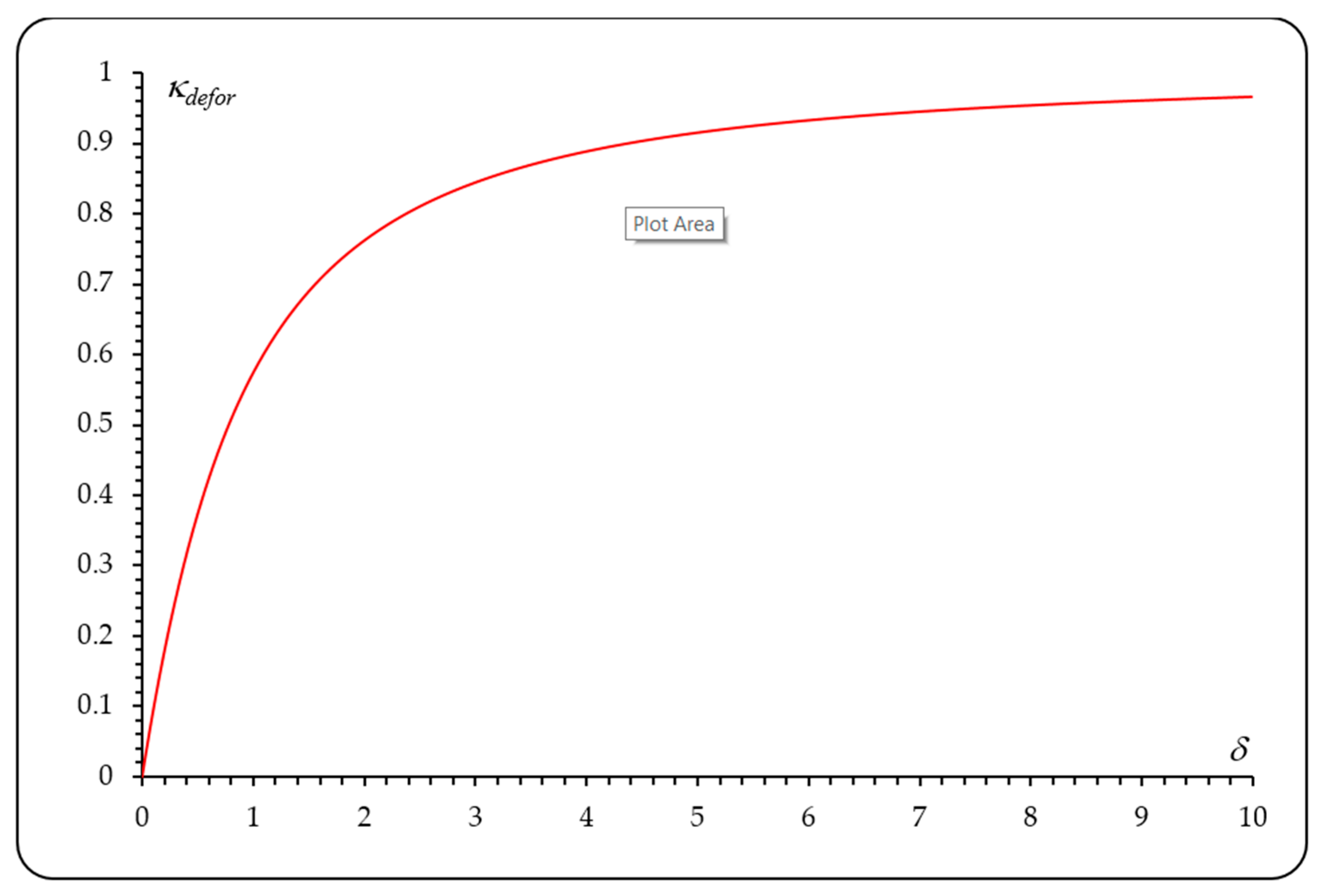
The Monte Carlo method was used to find functions κ_defor(δ) and κ’_defor(δ). Results of the applied stochastic calculations are shown in graphs in Figure 11 and Figure 12. Individual points of graphs were found by successive application of N = 10⁷ randomly chosen triples of variables {η⁽ⁱ⁾, χ⁽ⁱ⁾, S⁽ⁱ⁾} in Formulas (65) and (71). It was shown that with increasing number of applied random variables N the calculated values κ_defor and κ’_defor converge to some expected value of the degree of the whole grain- surface orientation for every value δ. This means that the computational stability of the Monte Carlo algorithm has been confirmed in the simulation of the relationship between orientation and deformation of the structure.

Results of the numerical calculation confirmed that Formulas (65) and (71) can be successfully applied for the conversion of the orientation represented by the quantity κ into local plastic deformation characterized by δ in the case of plastic deformation of the grained structure. In addition graphs κ_defor(δ) and κ’_defor(δ) obtained from these formulas using the Monte Carlo simulation demonstrate the applicability of stereological methods for the modelling of local plastic deformation in grained structures.

However, Formulas (65) and (71) do not represent a general solution. These results can only be applied to a particular case for which there is no rigid solid rotation of grains in the structure and the axes chosen are principal axes of strain (therefore, there are no shear components present). In addition, another limitation is imposed, which is that plastic deformation must be isotropic. Actually, it does not seem that a grain with anisotropic behavior would give complications in the practical implementation of our results.

8. Discussion and Conclusions

In our work we briefly pointed out the possible application of quantities obtained from standard stereological measurements. Our findings show that these quantities can be successfully applied for the modelling of local plastic deformation in grained structures. Our approach is based on the assumption that the grain, as it appears in a two-dimensional cross section, will change its shape and geometric orientation in 3D during plastic deformation. We applied and discussed our results for a homogeneous and isotropic grained structure.

The application is quite simple in the case of plastic deformation. The local plastic deformation in an isotropic and homogeneous grained structure can be evaluated by means of the value of grain elongation (or contraction) δ. However, the grain elongation (contraction) in the real structure cannot be measured directly. Conversely the measurement of the degree of grain orientation κ is available using stereological methods. One of the main benefits of our work is that we found the correlation between the degree of grain orientation κ and grain elongation (contraction) δ (see Formula (65) for elongation or (71) for contraction). A model of random grained structure was established and the mentioned correlation was investigated.

We note that by applying the Formulas (65) and (71), the correlations δ(κ) can be easily determined for various initial grained structure orientations represented by values κ_undefor. The initial orientation of a randomly selected grain in an undeformed random grained structure is arbitrary and κ_undefor = 0 in isotropic cases. However a relatively broad database of graphs {δ(κ, κ_undefor)} for the various κ_undefor could be calculated and recorded when using a computer technique. Subsequently, the value of grain elongation δ for corresponding κ can be found from the relevant graph. However, before this the graph for the quantification of δ must be selected from the database using the value κ_undefor measured for the undeformed configuration of the grained structure.

Therefore, if a deformation map of the plastically deformed homogeneous and isotropic grained structure is to be investigated in the future, we propose using the results obtained above by the procedure consisting of the following steps:

• The degree of grain orientation κ in some local area in the given i-th position in the grained structure must be measured in both undeformed (κⁱ_undefor) and deformed (κⁱ_defor) configurations. For example, the Saltykov stereological method is applicable for this purpose.
• Graph δ(κ) for a given model of grained structure must be identified so as the following is applied: δ (κⁱ_undefor) = 0. We found the graph for the random model of homogeneous and isotropic grained structure by applying the random matrix approximation (see Formulas (65) or (71)) and using Monte Carlo simulation (see Figure 11 and Figure 12). κⁱ_undefor = 0 was applied for the homogeneous isotropic case.
• Value δ_i corresponding to the measured value κⁱ_defor must be found only from the graph δ (κ). The search procedure is easy: δ_i = δ (κⁱ_defor). Finally, this value δ_i represents the grain elongation in the i-th position in the structure and allows the local strain in the given i-th position to be evaluated.

However if we have to discuss how the obtained results can be applied to the study of plastic deformation we must also note that the limitations imposed on Formulas (65) or (71) are often too strong to make the presented method useful to study real deformation processes. Namely, also rigid solid rotations of grains must be taken into account in general. Moreover, in order to be applicable in the field of crystal plasticity, the case of anisotropic grain behavior should be discussed. A more general method must be designed which does not lead to ambiguities in the interpretation of the change in the degree of grain orientation. In the general inhomogeneous and anisotropic case, the Formula (9) resulting from random matrix approximation should be used. This formula allows us to find the relationship between the measurable quantities κⁱ_defor and the coefficients of the deformation tensor ε_qm in the local area of the grained structure. However the degree of the grain orientation κ in the given local area of the grained structure will have to be measured in relation to more different vectors ${\overrightarrow{\tau }}^k$ (oriented in various directions) so that we get the appropriate number of equations corresponding to the number of unknown coefficients ε_qm. This means the next system of equations must be solved in the inhomogeneous and anisotropic case:

$${\kappa }_{defor}^k\approx 1-2\frac{{\displaystyle \sum _{i=1}^N\left(S^{\left(i\right)}\left|{\displaystyle \sum _{n=1}^3{\tau }_n^{k}det\left[{\tilde{A}}_n^{\left(i\right)}\left(\left\{{\epsilon }_{qm}\right\}\right)\right]}\right|\right)}}{{\displaystyle \sum _{i=1}^N\left(S_{}^{\left(i\right)}\sqrt{{\displaystyle \sum _{n=1}^3{\left(det\left[{\tilde{A}}_n^{\left(i\right)}\left(\left\{{\epsilon }_{qm}\right\}\right)\right]\right)}^2}}\right)}}q,m=1,2,3,k=1,2,9$$

(72)

Local values of the coefficients of the deformation tensor ε_qm can be determined from the system (73). In the case of plastic deformation one of the equations in the system () may be replaced by the Equation (47). Generally, the verification of the practical applicability of the suggested idea to determine local plastic deformation in a structure requires development of a suitable technique for experimental determination of κ_defor. Besides that, it is necessary to develop some numerical methods suitable for software processing that allow coefficients ε_qm to be found satisfying a system of Equation (73). System (73) quantified for ε_qm = δ_qm characterizes the initial orientation of the grained structure in relation tothe direction given by vectors ${\overrightarrow{\tau }}^k$ in the undeformed configuration and represents the initial conditions:

$${\kappa }_{undefor}^k\approx 1-2\frac{{\displaystyle \sum _{i=1}^N\left(S^{\left(i\right)}\left|{\displaystyle \sum _{n=1}^3{\tau }_n^{k}det\left[{\tilde{A}}_n^{\left(i\right)}\left(\left\{{\epsilon }_{qm}={\delta }_{qm}\right\}\right)\right]}\right|\right)}}{{\displaystyle \sum _{i=1}^N\left(S_{}^{\left(i\right)}\sqrt{{\displaystyle \sum _{n=1}^3{\left(det\left[{\tilde{A}}_n^{\left(i\right)}\left(\left\{{\epsilon }_{qm}={\delta }_{qm}\right\}\right)\right]\right)}^2}}\right)}}q,m=1,2,3,k=1,2,9$$

(73)

This initial condition must be considered in Equation (73) in the case of the deformed configuration and the deformation characteristics represented by tensor ε_qm in the local area of the grained structure can be searched by solving this system.

In conclusion, we dealt with the problem of applicability of stereological methods to determine local plastic deformation in a grained structure. One can easily understand that there is a correlation between the change in the grain orientation and grain deformation. This correlation was mathematically demonstrated in our work. Indeed, the expression (50) allows one to investigate this correlation. If the quantity κ clearly corresponds to the degree of grain orientation measured by the Saltykov method, the analysis of local deformation could be realized experimentally on the basis of our results. As an illustration we showed the applicability of our results for a random model of a grained structure. This specific model was used here because of its simplicity but we believe that our method can be applied also for other models.

During the loading process the κ changes and reflects deformation phenomena in the structure. On-line scanning of grain orientation could be of great help for in-situ investigation of the deformation dynamics. In this respect new methods for 3D object imaging may be helpful. Procedures for the practical realization of our method suggested above will have to be modified in this case and this modification will be the subject of a future work. However, we think that the mathematical principles of the method presented in our work will remain the same.

References

- Saltykov, S.A. Stereometric Metallography; Metallurgia: Moscow, Russia, 1970. [Google Scholar]
- Vander Voort, G.F. Measuring the grain size of specimens with non-equiaxed grains. Pract. Metallogr. 2013, 50, 239–251. [Google Scholar] [CrossRef]
- Maier, B.; Mihailova, B.; Paulmann, C.; Ihringer, J.; Gospodinov, M.; Stosch, R.; Güttler, B.; Bismayer, U. Effect of local elastic strain on the structure of Pb-based relaxors: A comparative study of pure and Ba- and Bi-doped PbSc0.5Nb0.5O3. Phys. Rev. 2009, 79, 224108. [Google Scholar] [CrossRef]
- Stoudt, M.R.; Levine, L.E.; Creuziger, A.; Hubbard, J.B. The fundamental relationships between grain orientation, deformation-induced surface roughness and strain localization in an aluminum alloy. Mater. Sci. Eng. A 2011, 530, 107–116. [Google Scholar] [CrossRef]
- Wang, X.G.; Witz, J.F.; El Bartali, A.; Dufrénoy, P.; Charkaluk, E. Investigation of grain-scale surface deformation of a pure aluminium polycrystal through kinematic-thermal full-field coupling measurement. In Proceedings of the 13th International Conference on Fracture, Beijing, China, 16–21 June 2013. [Google Scholar]
- Luong, M.P. Fatigue limit evaluation of metals using an infrared thermographic technique. I Mec. Mater. 1998, 28, 155–163. [Google Scholar] [CrossRef]
- Moscicki, M.; Kenesei, P.; Wright, J.; Pinto, H.; Lippmann, T.; Borbély, A.; Pyzalla, A.R. Friedels-pair based indexing method for characterization of single grains with hard X-rays. Mater. Sci. Eng. A 2009, 524, 64–68. [Google Scholar] [CrossRef]
- Deng, J.; Rokkam, S. A phase field model. of surface-energy-driven abnormal grain growth in thin films. Mater. Trans. 2011, 52, 2126–2130. [Google Scholar] [CrossRef]
- Gerth, D.; Schwarzer, R.A. Graphical Representation of grain and Hillock orientations in annealed Al-l%Si films. Textures Microstruct. 1993, 21, 77–93. [Google Scholar] [CrossRef] [Green Version]
- Sack, R.A. Indirect evaluation of orientation in polycrystalline materials. J. Polym. Sci. 1961, 51, 543–560. [Google Scholar] [CrossRef]
- Zhang, N.; Tong, W. An experimental study on grain deformation and interactions in an Al-0.5%Mg multicrystal. Int. J. Plast. 2004, 20, 523–542. [Google Scholar] [CrossRef]
- Lewis, H.D.; Walters, K.L.; Johnson, K.A. Particle size distribution by area analysis: Modifications and extensions of the Saltykov method. Metallography 1973, 6, 93–101. [Google Scholar] [CrossRef]
- Xu, Y.H.; Pitot, H.C. An improved stereologic method for three-dimensional estimation of particle size distribution from observations in two dimensions and its application. Comput. Methods Progr. Biomed. 2003, 72, 1–20. [Google Scholar] [CrossRef]
- Rayaprolu, D.B.; Jaffrey, D. Comparison of discrete particle sectioning correction methods based on section diameter and area. Metallography 1982, 15, 193–202. [Google Scholar] [CrossRef]
- Zhao, Z.; Ramesh, M.; Raabe, D.; Cuitiño, A.M.; Radovitzky, R. Investigation of three-dimensional aspects of grain-scale plastic surface deformation of an aluminum oligocrystal. Int. J. Plast. 2008, 24, 2278–2297. [Google Scholar] [CrossRef]
- Patdar, V. A Note on geometry of grain boundaries. Scr. Metal. 1986, 20, 1227–1230. [Google Scholar] [CrossRef]
- Bate, P.S.; Hutchinson, W.B. Grain boundary area and deformation. Scr. Mater. 2005, 52, 199–203. [Google Scholar] [CrossRef]
- Song, K.J.; Wei, Y.H.; Dong, Z.B.; Ma, R.; Zhan, X.H.; Zheng, W.J.; Fang, K. Constitutive model coupled with mechanical effect of volume change and transformation induced plasticity during solid phase transformation for TA15 alloy welding. Appl. Math. Modell. 2015, 39, 2064–2080. [Google Scholar] [CrossRef]
- Sharen, J.; Cummins, P.; Cleary, W. Using distributed contacts in DEM. Appl. Math. Modell. 2011, 35, 1904–1914. [Google Scholar]
- Singh, S.B.; Bhadeshia, H.K.D.H. Topology of grain deformation. Mater. Sci. Technol. 1998, 14, 832–834. [Google Scholar] [CrossRef]
- Yoshihiro, M.; Takayuki, S. Bayesian inference of whole-organ deformation dynamics from limited space-time point data. J. Theor. Biol. 2014, 357, 74–85. [Google Scholar]
- Sutton, M.A.; Orteu, J.J.; Schreier, H.W. Image Correlation for Shape, Motion and Deformation Measurements; Hardcover: Boston, MA, USA, 2009; ISBN 978-0-387-78746-6. [Google Scholar]
- Keating, T.J.; Wolf, P.R.; Scarpace, F.L. An improved method of digital image correlation. Photogramm. Eng. Remote Sens. 1975, 41, 993–1002. [Google Scholar]
- Gallucci Masteghin, M.; Ornaghi Orlandi, M. Grain-boundary resistance and nonlinear coefficient correlation for SnO2-based varistors. Mat. Res. 2016, 19, 1286–1291. [Google Scholar] [CrossRef] [Green Version]
- Sindre, B.; Knut, M.; Nes, E. Subgrain Structures Characterized by Electron. Backscatter Diffraction (EBSD). Mater. Sci. Forum 2014, 794, 3–8. [Google Scholar]
- Zou, H.F.; Zhang, Z.F. Application of electron backscatter diffraction to the study on orientation distribution of intermetallic compounds at heterogeneous interfaces (Sn/Ag and Sn/Cu). J. Appl. Phys. 2010, 108, 103518. [Google Scholar] [CrossRef]
- Zacher, G.; Paul, T. Research Applications. Qualitative and Quantitative Investigation of Soils and Porous Rocks by Using Very High Resolution X-Ray CT Imaging. Unsaturated Soils; Khalili, N., Russell, A., Khoshghalb, A., Eds.; Taylor & Francis Group: London, UK, 2014; ISBN 978-1-138-00150-3. [Google Scholar]
- Khalid, A.; Alshibli, A.; Reed, H. Advances in Computed Tomography for Geomaterials: GeoX 2010; John Wiley & Sons: Hoboken, NJ, USA, 2012. [Google Scholar]
- Bay, B.K.; Smith, T.S.; Fyhrie, D.P.; Saad, M. Digital volume correlation: Three-dimensional strain mapping using X-ray tomography. Exp. Mech. 1999, 39, 217–226. [Google Scholar] [CrossRef]
- Konrad, N.; Wenxiong, H. A study of localized deformation pattern in granular media. Comput. Methods Appl. Mech. Eng. 2004, 193, 2719–2743. [Google Scholar]
- Ronaldo, I.; Borja, A.A. Computational modeling of deformation bands in granular media. I. Geological and mathematical framework. Comput. Methods Appl. Mech. Eng. 2004, 193, 2667–2698. [Google Scholar]
- Wellmann, C.; Wriggers, P. A two-scale model of granular materials. Comput. Methods Appl. Mech. Eng. 2012, 205, 46–58. [Google Scholar] [CrossRef]
- Benedetti, I.; Aliabadi, M.H. A three-dimensional cohesive-frictional grain-boundary micromechanical model for intergranular degradation and failure in polycrystalline materials. Comput. Methods Appl. Mech. Eng. 2013, 265, 36–62. [Google Scholar] [CrossRef] [Green Version]
- Martinkovic, M.; Pokorny, P. Estimation of local plastic deformation in cutting zone during turning. Key Eng. Mater. 2015, 662, 173–176. [Google Scholar] [CrossRef]
- Martinkovic, M.; Minarik, S. Short notes on the grains modification by plastic deformation. In Plastic Deformation; Hubbard, D., Ed.; NOVA: New York, NY, USA, 2016; pp. 1–44. [Google Scholar]
- Takahashi, J.; Suito, H. Evaluation of the Accuracy of the Three-Dimensional Size Distribution Estimated from the Schwartz–Saltykov Method. Metall. Mater. Trans. A 2003, 34, 171–181. [Google Scholar] [CrossRef]
- Jensen, D. Estimation of the size distribution of spherical, disc-like or ellipsoidal particles in thin foils. J. Phys. D Appl. Phys. 1995, 28, 549. [Google Scholar] [CrossRef]
- Riosa, P.R.; Glicksmanb, M.E. Modeling polycrystals with regular polyhedra. Mater. Res. 2006, 9, 231–236. [Google Scholar] [CrossRef] [Green Version]
- Jae-Yong, C.; Qin, R.; Bhaeshia, H.K.D.H. Topology of the Deformation of a Non-uniform Grain Structure. ISIJ Int. 2009, 49, 115–118. [Google Scholar]
- Zhu, Q.; Sellars, C.M.; Bhadeshia, H.K.D.H. Quantitative metallography of deformed grains. Mater. Sci. Technol. 2007, 23, 757. [Google Scholar] [CrossRef]
Figure 1.
Test lines in the cutting plane at the linear orientation of the surfaces in the volume.
Figure 2.
Test lines in the cutting plane at the planar orientation of the surfaces in the volume.
Figure 3.
Test lines in the cutting planes at the linear-planar orientation of the surfaces in the volume.
Figure 4.
Scheme illustrating a view of an undeformed grained structure cross-section (for example on a metallographic cut). Scheme shows the cross-section of some individual grains.
Figure 5.
Scheme illustrating a view of the same grained structure cross-section in the deformed configuration. Scheme shows grain surfacedistortion and typical prolongation of grains.
Figure 6.
Undeformed grain.
Figure 7.
Deformed grain surface.
Figure 8.
A view of the single grain.
Figure 9.
Scheme illustrating a view of the model of the single grain.
Figure 10.
A view of a cross-section of the model of the grained structure. The scheme demonstrates cross-sectional images of small flat areas on the grain surface.
Figure 11.
Graph illustrating the result of Monte Carlo simulation of degree of orientation κ as a function of prolongation δ for a plastically deformed random grained structure. Vector is parallel to the deformation force.
Figure 12.
Graph illustrating the result of Monte Carlo simulation of degree of orientation κ as a function of contraction δ for plastically deformed random grained structure. Vector is perpendicular to the deformation force.
© 2020 by the authors. Licensee MDPI, Basel, Switzerland. This article is an open access article distributed under the terms and conditions of the Creative Commons Attribution (CC BY) license (http://creativecommons.org/licenses/by/4.0/).
Share and Cite
MDPI and ACS Style
Minárik, S.; Martinkovič, M. On the Applicability of Stereological Methods for the Modelling of a Local Plastic Deformation in Grained Structure: Mathematical Principles. Crystals 2020, 10, 697. https://doi.org/10.3390/cryst10080697
AMA Style
Minárik S, Martinkovič M. On the Applicability of Stereological Methods for the Modelling of a Local Plastic Deformation in Grained Structure: Mathematical Principles. Crystals. 2020; 10(8):697. https://doi.org/10.3390/cryst10080697
Chicago/Turabian StyleMinárik, Stanislav, and Maroš Martinkovič. 2020. "On the Applicability of Stereological Methods for the Modelling of a Local Plastic Deformation in Grained Structure: Mathematical Principles" Crystals 10, no. 8: 697. https://doi.org/10.3390/cryst10080697
Note that from the first issue of 2016, this journal uses article numbers instead of page numbers. See further details here.