
Addressing the Folding of Intermolecular Springs in Particle Simulations: Fixed Image Convention

School of Chemical Engineering, National Technical University of Athens (NTUA), GR-15780 Athens, Greece
*
Author to whom correspondence should be addressed.
Computation 2023, 11(6), 106; https://doi.org/10.3390/computation11060106
Submission received: 6 May 2023
/
Revised: 23 May 2023
/
Accepted: 24 May 2023
/
Published: 26 May 2023
(This article belongs to the Special Issue 10th Anniversary of Computation—Computational Chemistry)
Abstract
:Mesoscopic simulations of long polymer chains and soft matter systems are conducted routinely in the literature in order to assess the long-lived relaxation processes manifested in these systems. Coarse-grained chains are, however, prone to unphysical intercrossing due to their inherent softness. This issue can be resolved by introducing long intermolecular bonds (the so-called slip-springs) which restore these topological constraints. The separation vector of intermolecular bonds can be determined by enforcing the commonly adopted minimum image convention (MIC). Because these bonds are soft and long (ca 3–20 nm), subjecting the samples to extreme deformations can lead to topology violations when enforcing the MIC. We propose the fixed image convention (FIC) for determining the separation vectors of overextended bonds, which is more stable than the MIC and applicable to extreme deformations. The FIC is simple to implement and, in general, more efficient than the MIC. Side-by-side comparisons between the MIC and FIC demonstrate that, when using the FIC, the topology remains intact even in situations with extreme particle displacement and nonaffine deformation. The accuracy of these conventions is the same when applying affine deformation. The article is accompanied by the corresponding code for implementing the FIC.
1. Introduction
Understanding the structure–property relations in polymers and soft matter systems is key to designing advanced materials with tailor-made properties for applications in biology [1], nanocomposites [2,3,4,5], rheology [6,7,8], and more. Polymeric materials exhibit a rich spectrum of relaxation mechanisms, the longest of them spanning the millisecond to second regime, depending on the chain molar mass. The latter phenomena can be investigated with mesoscale simulation techniques such as Brownian dynamics [9] and dissipative particle dynamics [10,11], which treat large collections of atoms as single coarse-grained sites, in that manner drastically decreasing the degrees of freedom and affording huge savings in computational time.
Coarse-grained polymer chains are, however, prone to unphysical intercrossing, thus violating the network topology and yielding artificially faster dynamics and lower viscosity. Much research has been devoted to restoring the proper viscoelastic properties of coarse-grained polymers by enforcing the topological constraints in an artificial manner, such as the TWENTANGLEMENT model [12], and the slip-link [13,14] and slip-spring (SS) [15,16,17] models, all of them resting on the assumptions of reptation theory [18,19,20]. In the slip-spring model, the entanglements are modeled with entropic springs which are generated/destroyed at the chain ends and are able to slide along the chain contours during the course of the simulation, modeling in this way the mechanism of reptation. The slip-spring model has been particularly successful for restoring the viscoelastic properties of linear [8,17,21,22], star [23,24], and cross-linked [25,26,27] polymers, in bulk [8,17] and interfacial [5,21,28] geometries under quiescent and nonequilibrium [8,16,29,30] conditions.
A common boundary condition for investigating homogeneous samples is the periodic boundary condition (PBC), where the domain is treated as infinite along the periodic directions [9]. This is achieved by replicating the central box along these directions; these replicas are called box images. It is convenient to allow the particles to diffuse outside the central box in order to compute their transport properties. In doing so, the relative distance between two particles i and j (which may lie in different box images) can be corrected by enforcing a suitable convention such as the minimum image convention (MIC).
According to the MIC, each particle i interacts with the image of particle j that is closest to it, in such a way that the absolute projections of their separation vector on the basis vectors of the simulation box do not exceed half the corresponding edge lengths of the box. The MIC is applicable to non-orthogonal boxes as well, after adjusting for the shear displacement of the periodic images [9,31]. Care must be exercised, however, in the case of particle pairs connected by soft springs; in a situation where the spring projection on one or more of the coordinate axes exceeds half the box edge length along that axis, the separation vector is redefined with respect to the (new) closest pair of images of the particles, resulting in a violation of the system topology.
This issue can become especially prevalent in simulations of coarse-grained polymers that have been subjected to extreme deformation, due to the inherent softness of the intra- and intermolecular effective bonds (springs) involved. For example, the equilibrium length of the intermolecular springs that are used to mimic the entanglements (slip-springs [15,16]) is ca 3–20 nm [32]. Subjecting the system to strong flows can overextend the aforementioned bonds significantly and lead to topology violations. In addition, the stability of the simulation is severely affected during extensional flow experiments [33,34], due to the decreased cross-section of the sample which leads to frequent instabilities and topology violations. Another drawback of the MIC is that it entails considerable computational cost due to the calculation of remainders [9], whereas choosing an optimal algorithm depends on several factors such as the compiler optimization and processor architecture [35].
We propose an alternative convention for determining the separation vectors of molecular bonds, which we call the fixed image convention (FIC). In FIC, the MIC is enforced only once during the formation of the bond and the minimum separation vector is stored in memory, in terms of a shift vector. In subsequent iterations, the separation vector is calculated simply by adding a shift vector to the absolute separation vector. The FIC is applicable to boxes with either constant or varying size (i.e., simulations in the isothermal-isobaric ensemble). Note, however, that subjecting the system to affine deformation requires deforming the shift vectors as well. Given that the distance between the images is fixed, the system topology remains intact even for very large deformations. In general, this operation is much faster than the usual MIC, especially when working with non-orthogonal boxes.
The article is structured as follows: Section 2.1 illustrates the coordinate system used in this work, and Section 2.2 reports the formulation of the various conventions for determining the separation vector. Section 3.1 compares the accuracy of the MIC and the FIC under conditions of extreme displacement and affine/non-affine deformation. Section 3.2 assesses the stability of the conventions under random displacement and strong shear deformation. Section 3.3 discusses the efficiency of the MIC and the FIC. Finally, Section 4 summarizes the main findings of the work. The code for conducting the comparisons between the MIC and FIC is provided via a GitHub repository [36].
2. Methods
2.1. Coordinate System and Constraints
The edge vectors of a parallelepiped simulation box can be described according to Equation (1):
with Δxy, Δxz, and Δyz indicating the displacement of the y/z/z face along the x/x/y axis of an originally orthogonal box with dimensions Lx, Ly, and Lz. In addition, the shearing components can be constrained according to Equation (2):
Adding or subtracting multiples of the box edge vectors does not affect the magnitude of the separation vectors when enforcing suitable minimum image conventions [9]. The aforementioned restrictions impose no loss of generality; any set of arbitrary non-collinear edge vectors can be rotated, inverted, and translated in order to conform to these constraints. For convenience, we will refer to the configuration of a box with the vector:
2.2. Conventions of Separation Vectors
2.2.1. Absolute Distance (AD)
Let ri, rj denote the absolute position of two particles i, j. By absolute, it is meant that the particles may lie anywhere in the Cartesian domain regardless of the bounds of the box. Their absolute separation vector is defined according to Equation (4).
2.2.2. Minimum Image Convention (MIC)
In orthogonal boxes, the calculation of the minimum separation vector can be performed according to the MIC as follows:
with nint denoting the nearest integer rounding function, and a vector-valued function which returns the minimum image of a vector subject to the dimensions of an orthogonal periodic box, L.
In triclinic boxes, the minimum image vector is determined by applying the Lees–Edwards boundary condition [31], which requires a prerequisite step. Initially, one has to correct for the displacement of the periodic images [9]:
Subsequently, the minimum separation vector is retrieved by inputting to Equation (5):
2.2.3. Fixed Image Convention (FIC)
The FIC entails storing the difference between the minimum and the absolute separation vectors during the formation of the bond, in terms of the shift vector:
In the subsequent iterations, the separation vector is calculated simply by adding the absolute separation vector and the (constant) shift vector:
Deforming the box entails some additional operations. Let F be a linear transformer describing the mapping between a reference () and a transformed (v) vector:
with “ref” denoting the vectorial quantity before the deformation; details regarding the analytical calculation of F are reported in the Appendix A. Applying F to a parallelepiped transforms its edge vectors according to Equation (11).
Depending on the application [37], the coordinates of the constituent particles may or may not be transformed according to . According to the type of applied deformation, we have the following cases:
- Affine deformation: the transformation is applied to both the box and the constituent particles. In this case, the shift vectors are transformed accordingly:
- Nonaffine deformation: the transformation is applied only to the box, and the shift vectors remain unaffected:
Finally, in order to restart a simulation with the FIC, the shift vectors should be exported to the hard drive alongside the other properties of the simulation (box dimensions, coordinates, etc.) and be read during the restart procedure.
3. Results
3.1. Comparisons between MIC and FIC
We will first assess the accuracy of the MIC and FIC for the six representative scenarios (scn) that are depicted in Table 1. In each case, we apply a linear transformer to the box and/or the constituent particles which is related to the (nonsymmetrical) engineering strain tensor as follows:
Depending on whether the deformation has been applied to the box and/or the particle coordinates, we have the following cases: displacement (box, coord) = (F, T), nonaffine deformation (box, coord) = (T, F), and affine deformation (box, coord) = (T, T), with box and coord denoting Booleans.
In all cases, the particle i resides at the origin of the box; hence, it remains unaffected. The particle j has been placed in the first image of the box along the y-axis, mimicking in this manner the formation of a bond between two chains which reside in different periodic images. For simplicity, the calculations have been conducted in 2D; calculations in 3D yield similar qualitative findings.
3.1.1. Particle Displacement in Rigid Boxes
First, we will examine the effect of (over)extending an intermolecular bond connecting particles which lie in different periodic images of orthogonal boxes as a function of displacement.
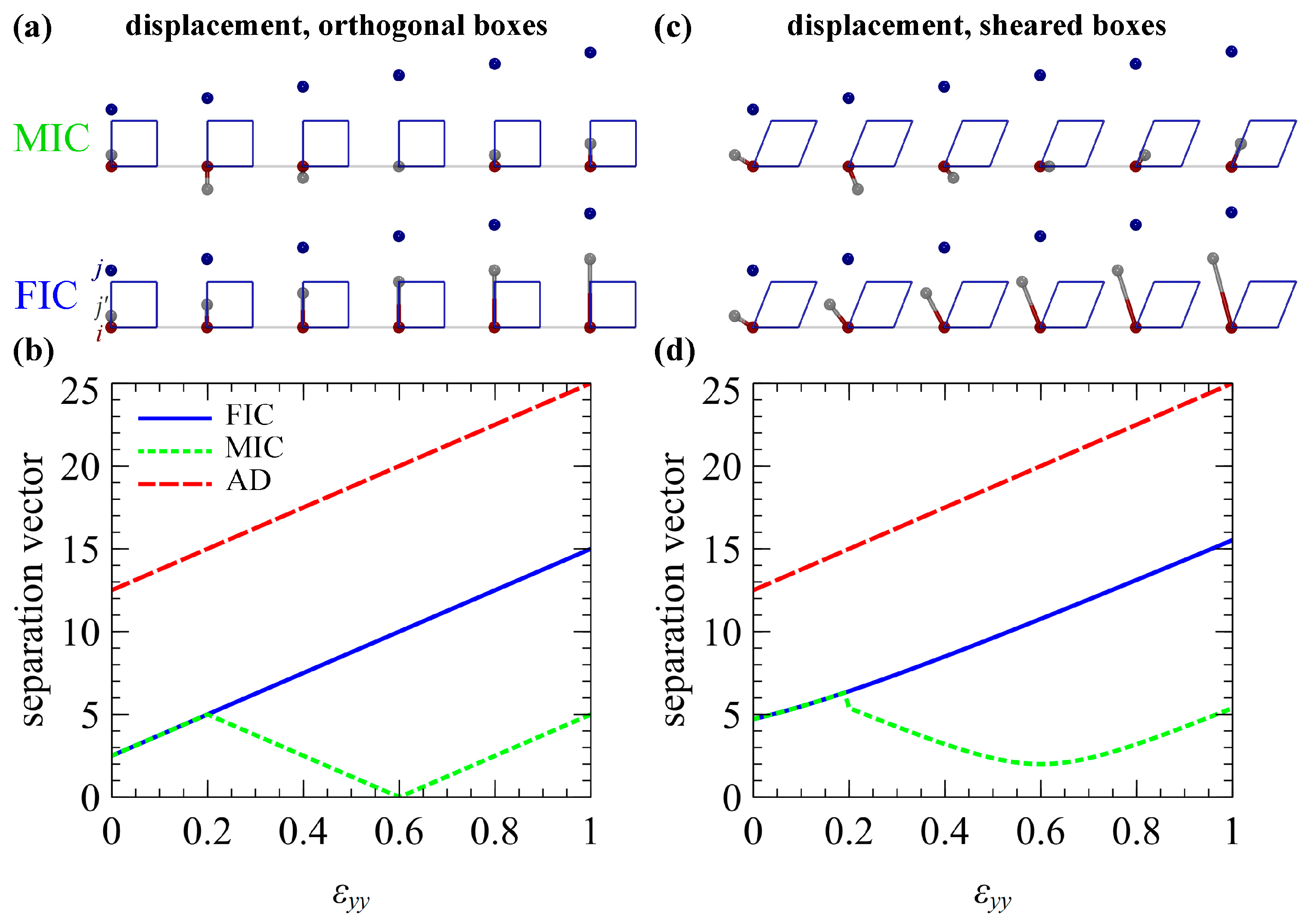
Figure 1a,b illustrate results from scenario A (see Table 1) where the particle j has been displaced with respect to particle i along the y-axis. In particular, Figure 1a illustrates snapshots of the particle positions and the separation vectors and connecting particle i with the image of particle j, hereafter referred to as . Figure 1b depicts the magnitude of the separation vectors (, , and ) as a function of the displacement in box units, i.e., Δy/Ly = εyy. For more details, please refer to the caption of Figure 1.
For small displacements (), the separation vectors according to the MIC and FIC are the same. For larger displacements (), the MIC becomes unstable since changes sign; i.e., the image of the particle in Figure 1a (MIC) hops to the −y image of the box. Instances such as this should be avoided during the course of practical simulations, since they violate the system topology. The FIC, on the other hand, yields the desired behavior, i.e., the separation vector increases proportionally with displacement.
Figure 1c,d depict the same evaluations but for a box that has been sheared along the x-axis (scenario B in Table 1). The behavior of the MIC and FIC is qualitatively the same as in the previous case; swaps signs and the image of the particle hops from the −x to the −y box image when , whereas increases steadily with the displacement.
3.1.2. Affine and Nonaffine Deformation (Varying Box Size)
In the following, we will examine the accuracy of the MIC and FIC during affine and nonaffine deformation experiments.
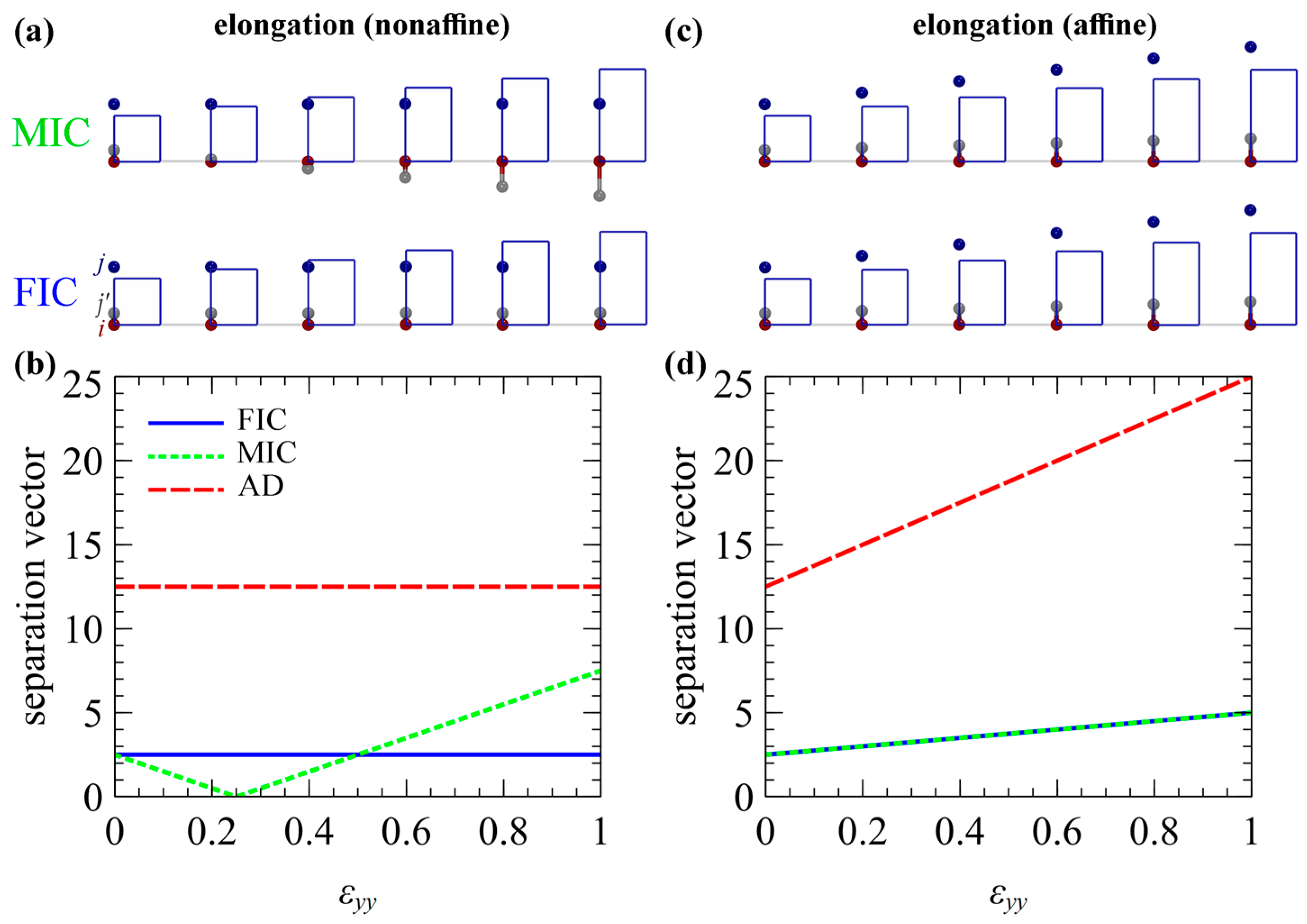
Figure 2 illustrates results from elongation experiments according to the parameters of scenarios C (panels a, b) and D (panels c, d) in Table 1; panels a, c illustrate snapshots of the system, and panels b, d show the magnitude of the separation vectors during the deformation according to the AD, MIC, and FIC.
According to Figure 2a,b, enforcing the FIC under nonaffine deformation conditions leaves the separation vector unchanged. Given that the relative positions of the particles are unchanged, it makes sense that the separation vector should remain the same. In contrast, enforcing the MIC results in some interesting behavior: decreases with increasing strain until Ly = rj, after which it increases indefinitely. Regardless, however, deforming the box while keeping the coordinates of the particles unchanged is not a well-defined process; thus, depending on the application, one may choose to apply either the MIC or the FIC.
Figure 2c,d present results from the same experiment, but with the difference that the particle coordinates are transformed along with the box (scn D in Table 1). In this situation, the MIC and FIC yield identical results. The projections of the separation vector change proportionally with the box dimensions; hence, they cannot become larger than half of the edge vectors of the box and swap box images.
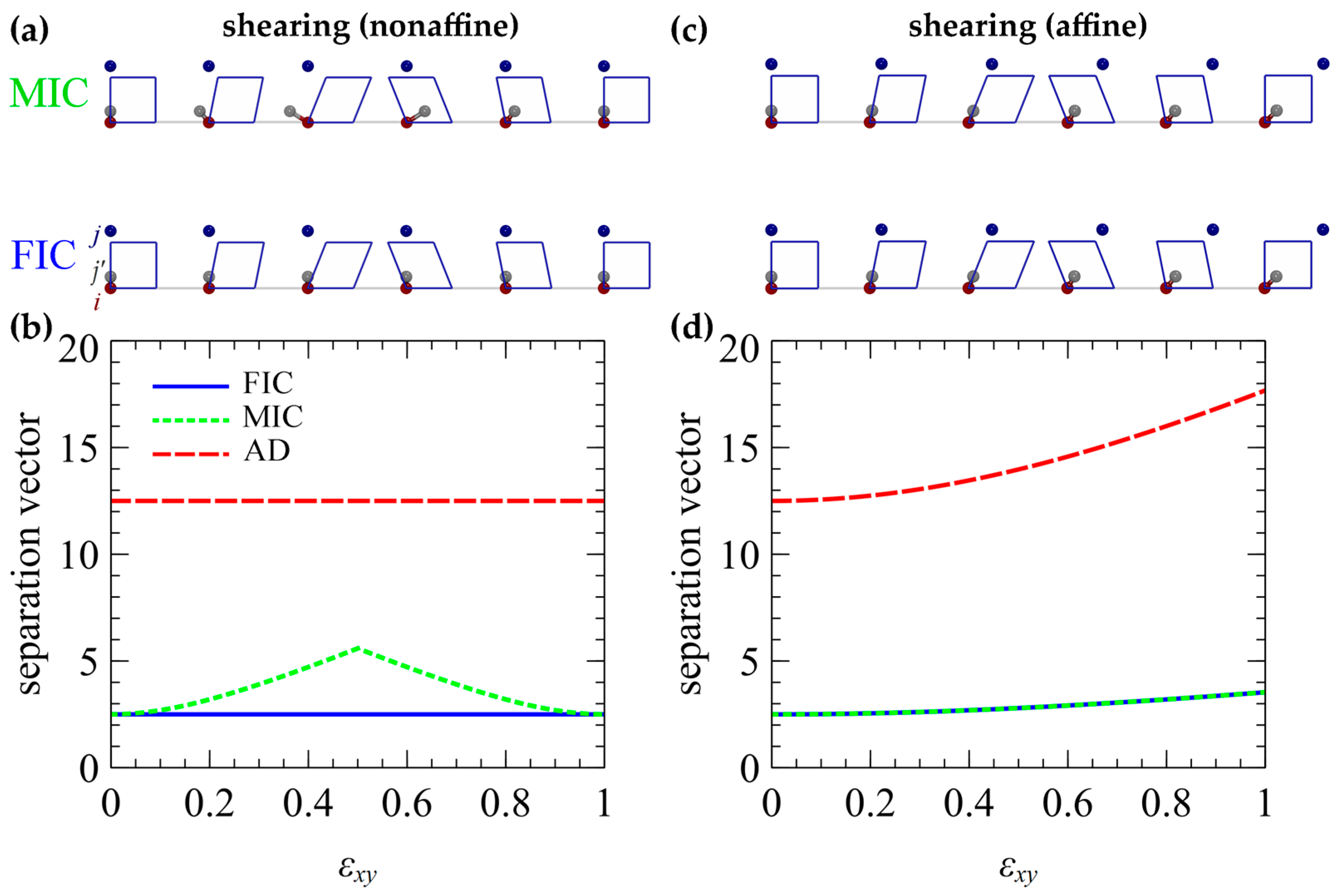
Figure 3 illustrates results from the shearing deformations according to scenarios E (panels a, b) and F (panels c, d) in Table 1. Note that at εxy = 0.5, Δxy flips sign according to the constraint in Equation (2). Similarly, with the nonaffine elongation experiments, enforcing the FIC leaves the separation vector unchanged, whereas the MIC results in complicated behavior. Under affine shear deformation conditions, the MIC and FIC result in identical behavior (Figure 3c,d).
3.2. Stability
In this section, we will assess the performance of the MIC and FIC against bead-spring molecular mechanics models under conditions of extreme deformation.
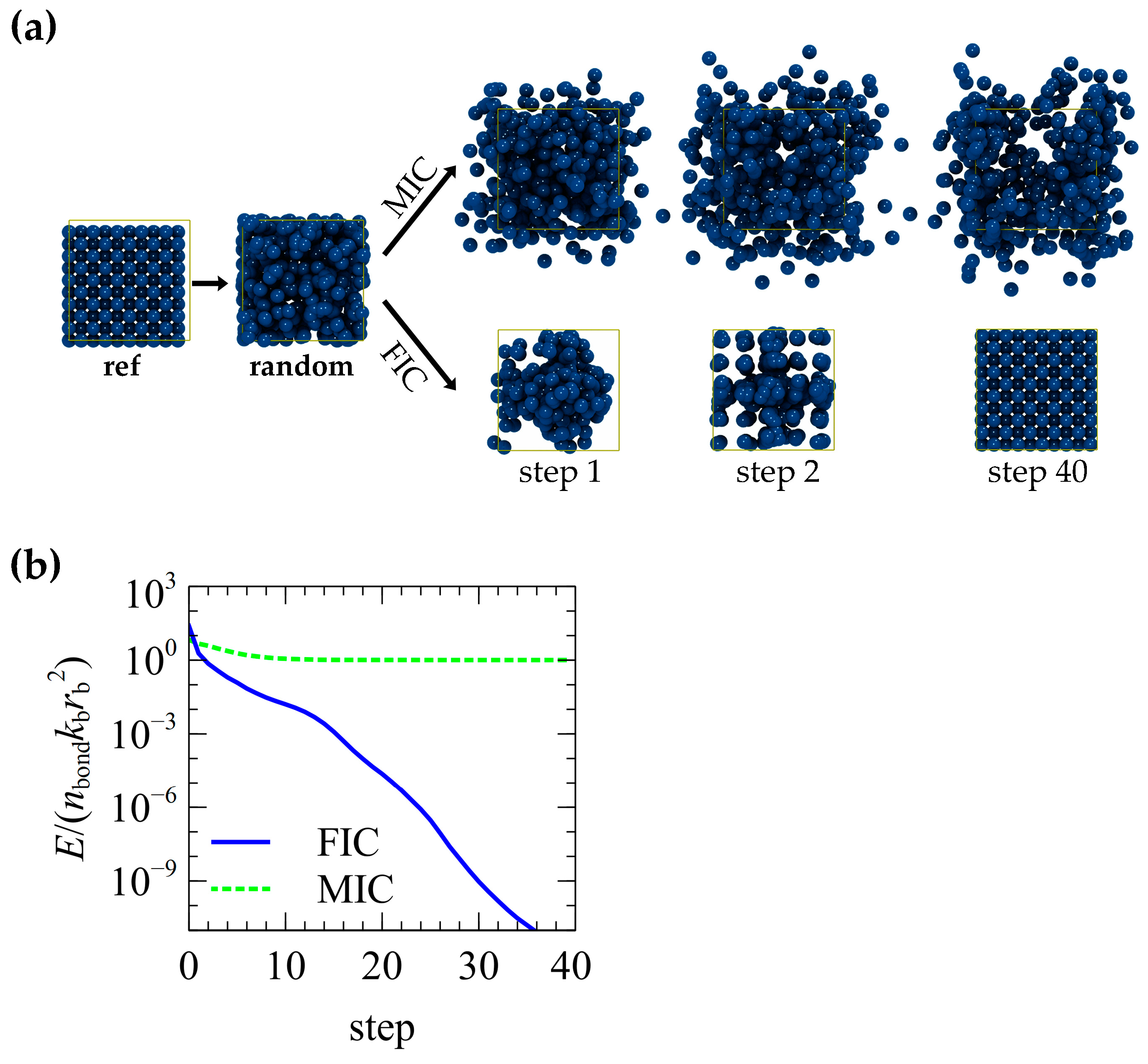
Figure 4a (left) depicts a periodic face-centered cubic (FCC) lattice made by 5 × 5 × 5, four-particle unit cells with lattice constant, acell = 10 Å. Each particle interacts with its 12 nearest neighbors (nbond = 3000 total interactions) via a harmonic potential of the form:
where kb = 10−5 kJ/(molÅ2), and is the first neighbor distance. The particles at the periodic boundaries interact with their nearest images subject to the MIC or the FIC; thus, the energy of this reference state is zero.
The particle coordinates are randomized and the configuration is subjected to an energy minimization via a conjugate gradient algorithm [38,39] that has been implemented in the EMSiPoN code [8,17,25,28] (see Appendix B). The evolution of the normalized energy during the course of the minimization is illustrated in Figure 4b. The FIC yields a higher energy at the start of the optimization (Figure 4b, step = 0) because it describes the topology of the overextended bonds properly. The initial energy is lower when enforcing the MIC because the topology is violated since the separation vectors are redefined with respect to the (new) nearest image particles. Due to these topology violations, the MIC performs rather poorly, and the system cannot return to its initial state. In contrast, the FIC keeps the topology intact, and the system is able to return to its initial state after the minimization.
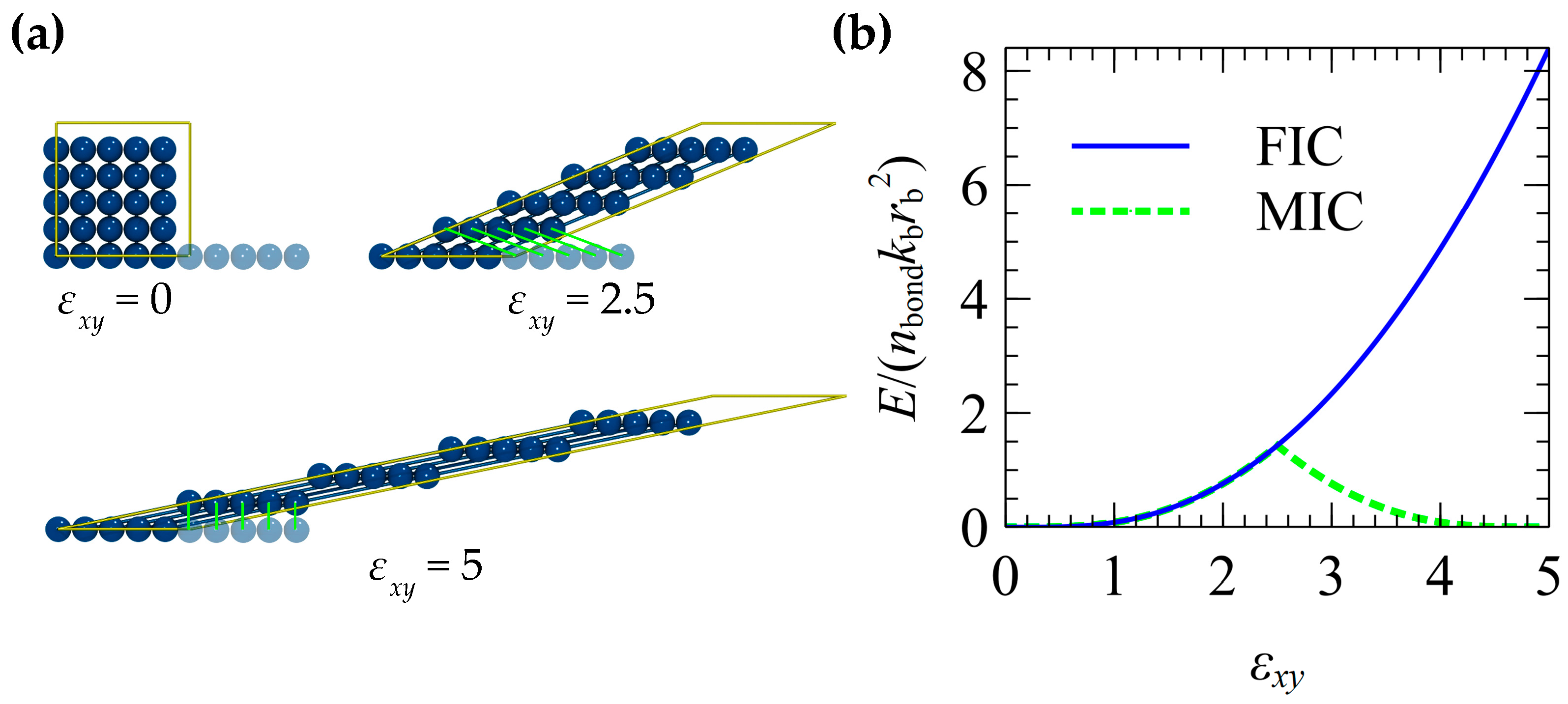
Figure 5a (panel εxy = 0) depicts a periodic 5 × 5 square lattice with alat = 2 Å. Each particle interacts with its four closest neighbors (nbond = 50) according to Equation (15) with kb = 1 kJ/mol and rb = alat. The lattice is gradually sheared along the x-axis for εxy up to 5; the evolution of the normalized energy during this operation is shown in Figure 5b.
For shear deformations up to εxy = 2.5, the energy increases parabolically, regardless of the image convention. After this threshold, the ends of the vector attach to the image particles in the +x box image; see green bonds in Figure 5a. As a result, the energy starts to decrease with increasing strain, whereas at εxy = 5, the system returns to its initial (undeformed) state. When enforcing the FIC, on the other hand, the energy increases indefinitely with increasing strain, indicating that the extreme shear displacement is described properly.
3.3. Efficiency
The implementation of the MIC entails increased computational cost due to the calculation of the remainders in Equation (5); the computational time increases further when working with nonorthogonal boxes (see Equation (6)) due to the correction for shear displacement. Several algorithms have been proposed in the literature for enforcing the MIC [9,35]. Choosing an optimal algorithm depends on several factors such as the processor architecture and the compiler optimizations [35].
The FIC is generally cheaper since it requires adding a shift vector to the absolute separation vector. The shift vectors are computed only once during the formation of the bond and are stored in memory. The additional burden on system memory scales as O(n); it is negligible considering the modern computer architectures. It is worth mentioning that, in cases where the system is subjected to affine deformation, the shift vectors must be transformed according to Equation (12), thus increasing the cost of the operation slightly.
4. Conclusions
We have developed the fixed image convention (FIC) for determining the separation vectors of the intra- and intermolecular (effective) bonds in particle simulations. The accuracy of the FIC has been assessed in terms of conducting comparisons with the commonly adopted minimum image convention (MIC). The experiments for particle displacement and nonaffine deformation demonstrate that, when the projections of the separation vectors exceed half of the box projections, the minimum image separation vector swaps periodic images, and in this manner, the topology of the system is violated. The FIC, on the other hand, keeps the topology of the system intact, even at extreme deformations. Subjecting the system to affine deformation (i.e., applying the linear transformer to both the box vectors and particle coordinates) yields the same (stable) behavior, regardless of the convention. Given that in the FIC the separation vectors between the images are fixed, the system is able to return to its initial (undeformed) state regardless of how it is deformed. The computational cost for enforcing the FIC is generally lower than that of the MIC. The FIC is generic and applicable to several types of particle-based simulations and bonding schemes.
Author Contributions
Conceptualization, A.P.S. and D.N.T.; methodology, A.P.S.; software, A.P.S.; validation, A.P.S.; formal analysis, A.P.S.; investigation, A.P.S. and D.N.T.; resources, D.N.T.; data curation, A.P.S.; writing—original draft preparation, A.P.S.; writing—review and editing, A.P.S. and D.N.T.; visualization, A.P.S.; supervision, D.N.T.; project administration, A.P.S. and D.N.T.; funding acquisition, D.N.T. All authors have read and agreed to the published version of the manuscript.
Funding
This research was funded by SOLVAY.
Data Availability Statement
The source code for conducting the experiments shown in Table 1 can be accessed via the GitHub repository: https://github.com/ArisSgouros/FixImag.git (accessed on 22 May 2023).
Acknowledgments
The authors thank Constantinos J. Revelas for the fruitful discussions regarding the determination of the deformation gradient tensor from the reference and transformed box vectors.
Conflicts of Interest
The authors declare no conflict of interest. The funders had no role in the design of the study; in the collection, analyses, or interpretation of data; in the writing of the manuscript; or in the decision to publish the results.
Appendix A. Analytic Expression of the Deformation Gradient
In the general case, the deformation gradient F satisfies the following equations:
with [] and [] being two sets with non-collinear vectors. In matrix representation, Equation (A1) can be expressed as follows:
or
with being a vectorial representation of . Solving entails inversing the matrix M:
In terms of the restricted coordinate system presented in Section 2.1 (y1 = z1 = z2 = = = = 0), the components of the deformation gradient can be obtained analytically according to Equation (A5).
Appendix B. Implementation of a Conjugate Gradient Algorithm
Given an objective function A(r) with known gradient , the first can be minimized iteratively as:
where dk is the search direction, and αk is the (scalar) step size. At the first step, dk is set to −gk.
At each iteration, ak is optimized via a three-stage linear search keeping dk, rk constant:
- Bracket minimum between two larger values;
- Optimize ak via inverse parabolic interpolation;
- In case (ii) fails, switch to the golden-section optimization.
To speed up the linear search, the initial guess of ak is updated in the following manner:
with being a learning rate. Note that the force is not calculated during the aforementioned linear search.
Upon completion of the linear search, in case of convergence, the process is terminated. The conditions for convergence are the following:
- The absolute difference between the current (Enext) and previous (Eprev) energy is below a tolerance value:
- A maximum minimization step (kmax) has been exceeded.
If the convergence has not been achieved, we proceed and compute the new forces based on the new configuration rk+1:
The search direction is then updated according to the following rule:
is the conjugate gradient parameter and can be calculated either from the Fletcher–Reeves formula [38]:
or from the Polak–Ribière formula [39]:
The aforementioned process is repeated from the start until convergence.
In the minimizations reported in Figure 4, the parameters of the optimization are the following: ΔEtol = 10−15 kJ/mol, kmax = 40, ak_init = 0.5, alearn = 0.5.
References
- Bernaschi, M.; Melchionna, S.; Succi, S. Mesoscopic Simulations at the Physics-Chemistry-Biology Interface. Rev. Mod. Phys. 2019, 91, 25004. [Google Scholar] [CrossRef]
- Zeng, Q.H.; Yu, A.B.; Lu, G.Q. Multiscale Modeling and Simulation of Polymer Nanocomposites. Prog. Polym. Sci. 2008, 33, 191–269. [Google Scholar] [CrossRef]
- Langner, K.M.; Sevink, G.J.A. Mesoscale Modeling of Block Copolymer Nanocomposites. Soft Matter 2012, 8, 5102–5118. [Google Scholar] [CrossRef]
- Lyulin, S.V.; Larin, S.V.; Nazarychev, V.M.; Fal’kovich, S.G.; Kenny, J.M. Multiscale Computer Simulation of Polymer Nanocomposites Based on Thermoplastics. Polym. Sci. Ser. C 2016, 58, 2–15. [Google Scholar] [CrossRef]
- Sgouros, A.P.; Vogiatzis, G.G.; Megariotis, G.; Tzoumanekas, C.; Theodorou, D.N. Multiscale Simulations of Graphite-Capped Polyethylene Melts: Brownian Dynamics/Kinetic Monte Carlo Compared to Atomistic Calculations and Experiment. Macromolecules 2019, 52, 7503–7523. [Google Scholar] [CrossRef]
- Padding, J.T.; Briels, W.J.; Stukan, M.R.; Boek, E.S. Review of Multi-Scale Particulate Simulation of the Rheology of Wormlike Micellar Fluids. Soft Matter 2009, 5, 4367–4375. [Google Scholar] [CrossRef]
- Nafar Sefiddashti, M.H.; Edwards, B.J.; Khomami, B. Individual Chain Dynamics of a Polyethylene Melt Undergoing Steady Shear Flow. J. Rheol. 2015, 59, 119–153. [Google Scholar] [CrossRef]
- Sgouros, A.P.; Megariotis, G.; Theodorou, D.N. Slip-Spring Model for the Linear and Nonlinear Viscoelastic Properties of Molten Polyethylene Derived from Atomistic Simulations. Macromolecules 2017, 50, 4524–4541. [Google Scholar] [CrossRef]
- Allen, M.P.; Tildeslay, D.J. Computer Simulation of Liquids; Clarendon Press: New York, NY, USA, 1989; ISBN 0198556454. [Google Scholar]
- Groot, R.D.; Warren, P.B. Dissipative Particle Dynamics: Bridging the Gap between Atomistic and Mesoscopic Simulation. J. Chem. Phys. 1997, 107, 4423–4435. [Google Scholar] [CrossRef]
- Español, P.; Warren, P.B. Perspective: Dissipative Particle Dynamics. J. Chem. Phys. 2017, 146, 150901. [Google Scholar] [CrossRef]
- Padding, J.T.; Briels, W.J. Time and Length Scales of Polymer Melts Studied by Coarse-Grained Molecular Dynamics Simulations. J. Chem. Phys. 2002, 117, 925–943. [Google Scholar] [CrossRef]
- Schieber, J.D.; Neergaard, J.; Gupta, S. A Full-Chain, Temporary Network Model with Sliplinks, Chain-Length Fluctuations, Chain Connectivity and Chain Stretching. J. Rheol. 2003, 47, 213. [Google Scholar] [CrossRef]
- Nair, D.M.; Schieber, J.D. Linear Viscoelastic Predictions of a Consistently Unconstrained Brownian Slip-Link Model. Macromolecules 2006, 39, 3386–3397. [Google Scholar] [CrossRef]
- Likhtman, A.E. Single-Chain Slip-Link Model of Entangled Polymers: Simultaneous Description of Neutron Spin-Echo, Rheology, and Diffusion. Macromolecules 2005, 38, 6128–6139. [Google Scholar] [CrossRef]
- Masubuchi, Y. Simulating the Flow of Entangled Polymers. Annu. Rev. Chem. Biomol. Eng. 2014, 5, 11–33. [Google Scholar] [CrossRef]
- Vogiatzis, G.G.; Megariotis, G.; Theodorou, D.N. Equation of State-Based Slip-Spring Model for Entangled Polymer Dynamics. Macromolecules 2017, 50, 3004–3029. [Google Scholar] [CrossRef]
- Edwards, S.F. The Statistical Mechanics of Polymerized Material. Proc. Phys. Soc. 1967, 92, 9–16. [Google Scholar] [CrossRef]
- de Gennes, P.G. Reptation of a Polymer Chain in the Presence of Fixed Obstacles. J. Chem. Phys. 1971, 55, 572. [Google Scholar] [CrossRef]
- Doi, M. Explanation for the 3.4-Power Law for Viscosity of Polymeric Liquids on the Basis of the Tube Model. J. Polym. Sci. Polym. Phys. Ed. 1983, 21, 667–684. [Google Scholar] [CrossRef]
- Ramírez-Hernández, A.; Peters, B.L.; Schneider, L.; Andreev, M.; Schieber, J.D.; Müller, M.; de Pablo, J.J. A Multi-Chain Polymer Slip-Spring Model with Fluctuating Number of Entanglements: Density Fluctuations, Confinement, and Phase Separation. J. Chem. Phys. 2017, 146, 014903. [Google Scholar] [CrossRef]
- Masubuchi, Y.; Doi, Y.; Uneyama, T. Effects of Slip-Spring Parameters and Rouse Bead Density on Polymer Dynamics in Multichain Slip-Spring Simulations. J. Phys. Chem. B 2022, 126, 2930–2941. [Google Scholar] [CrossRef] [PubMed]
- Masubuchi, Y. Multi-Chain Slip-Spring Simulations for Branch Polymers. Macromolecules 2018, 51, 10184–10193. [Google Scholar] [CrossRef]
- Philippas, A.P.; Sgouros, A.P.; Megariotis, G.; Theodorou, D.N. Mesoscopic Simulations of Star Polyethylene Melts at Equilibrium and under Steady Shear Flow. In Proceedings of the International Conference of Computational Methods in Sciences and Engineering ICCMSE 2020, Crete, Greece, 29 April–3 May 2020; Volume 2343. [Google Scholar] [CrossRef]
- Megariotis, G.; Vogiatzis, G.G.; Sgouros, A.P.; Theodorou, D.N. Slip Spring-Based Mesoscopic Simulations of Polymer Networks: Methodology and the Corresponding Computational Code. Polymers 2018, 10, 1156. [Google Scholar] [CrossRef] [PubMed]
- Masubuchi, Y.; Uneyama, T. Retardation of the Reaction Kinetics of Polymers Due to Entanglement in the Post-Gel Stage in Multi-Chain Slip-Spring Simulations. Soft Matter 2019, 15, 5109–5115. [Google Scholar] [CrossRef] [PubMed]
- Schneider, J.; Fleck, F.; Karimi-Varzaneh, H.A.; Müller-Plathe, F. Simulation of Elastomers by Slip-Spring Dissipative Particle Dynamics. Macromolecules 2021, 54, 5155–5166. [Google Scholar] [CrossRef]
- Sgouros, A.P.; Lakkas, A.T.; Megariotis, G.; Theodorou, D.N. Mesoscopic Simulations of Free Surfaces of Molten Polyethylene: Brownian Dynamics/Kinetic Monte Carlo Coupled with Square Gradient Theory and Compared to Atomistic Calculations and Experiment. Macromolecules 2018, 51, 9798–9815. [Google Scholar] [CrossRef]
- Chappa, V.C.; Morse, D.C.; Zippelius, A.; Müller, M. Translationally Invariant Slip-Spring Model for Entangled Polymer Dynamics. Phys. Rev. Lett. 2012, 109, 148302. [Google Scholar] [CrossRef]
- Moghadam, S.; Saha Dalal, I.; Larson, R.G. Slip-Spring and Kink Dynamics Models for Fast Extensional Flow of Entangled Polymeric Fluids. Polymers 2019, 11, 465. [Google Scholar] [CrossRef]
- Lees, A.W.; Edwards, S.F. The Computer Study of Transport Processes under Extreme Conditions. J. Phys. C Solid State Phys. 1972, 5, 1921–1928. [Google Scholar] [CrossRef]
- Fetters, L.J.; Lohse, D.J.; Colby, R.H. CHAPTER 25 Chain Dimensions and Entanglement Spacings. In Physical Properties of Polymers Handbook; Springer: Berlin/Heidelberg, Germany, 2006; pp. 445–452. [Google Scholar] [CrossRef]
- Petrie, C.J.S. Extensional Flow—A Mathematical Perspective. Rheol. Acta 1995, 34, 12–26. [Google Scholar] [CrossRef]
- Petrie, C.J.S. One Hundred Years of Extensional Flow. J. Nonnewton. Fluid Mech. 2006, 137, 1–14. [Google Scholar] [CrossRef]
- Deiters, U.K. Efficient Coding of the Minimum Image Convention. Z. Phys. Chem. 2013, 227, 345–352. [Google Scholar] [CrossRef]
- Sgouros, P.A.; Theodorou, D.N. FixImag. Available online: https://github.com/ArisSgouros/FixImag.git (accessed on 22 May 2023).
- Thompson, A.P.; Aktulga, H.M.; Berger, R.; Bolintineanu, D.S.; Brown, W.M.; Crozier, P.S.; in ’t Veld, P.J.; Kohlmeyer, A.; Moore, S.G.; Nguyen, T.D.; et al. LAMMPS—A Flexible Simulation Tool for Particle-Based Materials Modeling at the Atomic, Meso, and Continuum Scales. Comput. Phys. Commun. 2022, 271, 108171. [Google Scholar] [CrossRef]
- Fletcher, R.; Reeves, C.M. Function Minimization by Conjugate Gradients. Comput. J. 1964, 7, 149–154. [Google Scholar] [CrossRef]
- Polak, E.; Ribière, G. Note sur la convergence de méthodes de directions conjuguées. ESAIM Math. Model. Numer. Anal. Modélisation Mathématique Anal. Numérique 1969, 3, 35–43. [Google Scholar] [CrossRef]
Figure 1.
(a,c) Snapshots of the box edges and particle positions (i, red; j, blue; , grey) during the deformation at strain increments of 0.2. The grey bead depicts the image () of j that is bonded to particle i according to the MIC (top) or FIC (bottom). (b,d) Magnitude of the separation vectors according to the AD (dashes), MIC (dots), and FIC (solid). Panels (a,b) and (c,d) correspond to scenarios A and B in Table 1, respectively.


Figure 4.
(a) Snapshots of the energy minimization of an originally undeformed FCC crystal (ref) with 5 × 5 × 5 unit cells, by enforcing the MIC (top row) or the FIC (bottom row). Steps refer to iterations of the conjugate gradient algorithm. (b) Evolution of the normalized energy during the minimization.

Figure 5.
(a) Illustration of a shear deformation experiment of a periodic square lattice with alat = 2 Å for shear strain up to εxy = 5. The transparent particles correspond to the first layer of the image particles in the +x image of the box. The green lines indicate the formation of new bonds with the transparent layer of image particles when enforcing the MIC. For clarity, the constraint to Δxy according to Equation (2) has not been applied to these visualizations and the box is sheared continuously. (b) Evolution of the normalized energy during the shear experiment.


Table 1.
Parameters of scenarios A–F. The columns under the operation header denote the components of the maximum applied strain tensor (Equation (14)) and whether the transformation has been applied to the box and/or the particle positions. The columns under the reference/deformed header correspond to the dimensions of the box and the magnitude of the separation vectors before/after the deformation *.
| scn | Operation | Reference | Deformed | |||||||||||
|---|---|---|---|---|---|---|---|---|---|---|---|---|---|---|
| εyy | εxy | box | coord | |||||||||||
| A | 1 | 0 | F | T | 10 | 0 | 12.5 | 2.5 | 2.5 | 10 | 0 | 25 | 5 | 15 |
| B | 1 | 0 | F | T | 10 | 4 | 12.5 | 4.71 | 4.71 | 10 | 4 | 25 | 5.38 | 15.52 |
| C | 1 | 0 | T | F | 10 | 0 | 12.5 | 2.5 | 2.5 | 20 | 0 | 12.5 | 7.5 | 2.5 |
| D | 1 | 0 | T | T | 10 | 0 | 12.5 | 2.5 | 2.5 | 20 | 0 | 25 | 5 | 5 |
| E | 0 | 1 | T | F | 10 | 0 | 12.5 | 2.5 | 2.5 | 10 | 5 | 12.5 | 2.5 | 2.5 |
| F | 0 | 1 | T | T | 10 | 0 | 12.5 | 2.5 | 2.5 | 10 | 5 | 17.67 | 3.53 | 3.53 |
* In all cases: εxx = εyx = 0; ; , .
Disclaimer/Publisher’s Note: The statements, opinions and data contained in all publications are solely those of the individual author(s) and contributor(s) and not of MDPI and/or the editor(s). MDPI and/or the editor(s) disclaim responsibility for any injury to people or property resulting from any ideas, methods, instructions or products referred to in the content. |
© 2023 by the authors. Licensee MDPI, Basel, Switzerland. This article is an open access article distributed under the terms and conditions of the Creative Commons Attribution (CC BY) license (https://creativecommons.org/licenses/by/4.0/).
Share and Cite
MDPI and ACS Style
Sgouros, A.P.; Theodorou, D.N. Addressing the Folding of Intermolecular Springs in Particle Simulations: Fixed Image Convention. Computation 2023, 11, 106. https://doi.org/10.3390/computation11060106
AMA Style
Sgouros AP, Theodorou DN. Addressing the Folding of Intermolecular Springs in Particle Simulations: Fixed Image Convention. Computation. 2023; 11(6):106. https://doi.org/10.3390/computation11060106
Chicago/Turabian StyleSgouros, Aristotelis P., and Doros N. Theodorou. 2023. "Addressing the Folding of Intermolecular Springs in Particle Simulations: Fixed Image Convention" Computation 11, no. 6: 106. https://doi.org/10.3390/computation11060106
Note that from the first issue of 2016, this journal uses article numbers instead of page numbers. See further details here.