
Air Pollution and Climate Drive Annual Growth in Ponderosa Pine Trees in Southern California

Department of Environmental Studies, University of Redlands, 1200 E. Colton Avenue, Redlands, CA 92374, USA
Climate 2021, 9(5), 82; https://doi.org/10.3390/cli9050082
Submission received: 29 March 2021
/
Revised: 22 April 2021
/
Accepted: 7 May 2021
/
Published: 13 May 2021
(This article belongs to the Special Issue Climate Change Impact on Plant Ecology)
Abstract
:The ponderosa pine (Pinus ponderosa, Douglas ex C. Lawson) is a climate-sensitive tree species dominant in the mixed conifer stands of the San Bernardino Mountains of California. However, the close proximity to the city of Los Angeles has resulted in extremely high levels of air pollution. Nitrogen (N) deposition, resulting from nitrous oxides emitted from incomplete combustion of fossil fuels, has been recorded in this region since the 1980s. The impact of this N deposition on ponderosa pine growth is complex and often obscured by other stressors including climate, bark beetle attack, and tropospheric ozone pollution. Here I use a 160-year-long (1855–2015) ponderosa pine tree ring chronology to examine the annual response of tree growth to both N deposition and climate in this region. The chronology is generated from 34 tree cores taken near Crestline, CA. A stepwise multiple regression between the tree ring chronology and various climate and air pollution stressors indicates that drought conditions at the end of the rainy season (March) and NO2 pollution during the water year (pOct-Sep) exhibit primary controls on growth (r2-adj = 0.65, p < 0.001). The direct correlation between NO2 and tree growth suggests that N deposition has a positive impact on ponderosa pine bole growth in this region. However, it is important to note that ozone, a known stressor to ponderosa pine trees, and NO2 are also highly correlated (r = 0.84, p < 0.05). Chronic exposure to both ozone and nitrogen dioxide may, therefore, have unexpected impacts on tree sensitivity to climate and other stressors in a warming world.
1. Introduction
The ponderosa pine (Pinus ponderosa, Douglas ex C. Lawson) has long been used as a proxy for climate information in the American Southwest [1,2,3]. Tree ring growth in this seminal species has been found to be sensitive to changes in precipitation [4,5,6], water availability [7], the El Niño Southern Oscillation [8,9], and drought [10]. However, most of these studies have been conducted in the Sierra Nevada, where ponderosa pine trees dominate the interior forest of that region [11]. Fewer chronologies have been used to understand the climate sensitivity of ponderosa pine trees growing in the San Bernardino Mountains of Southern California, where the species is dominant at higher elevations (1524–2438 m) in mixed conifer stands. The region is located in a Mediterranean climate [12] where the wind flow pattern is driven by local topography, island configuration, proximity to the Pacific Ocean, and the semipermanent high pressure of the Northeastern Pacific [13,14,15,16,17,18]. These factors generate a strong sea breeze of westerly onshore flow that is present throughout the year, denominated by the Catalina eddies that grow in MAM and peak during the summer season (JJA) [19]. The climate of the region is distinct from the Sierra Nevada to the North. While mean annual temperature is similar between these two mountain regions (12–14 °C), the high Sierras (>1500 m) experience much greater rainfall (1778–2032 mm) than the Transverse Ranges (824 mm). Despite this difference, of the 32 ponderosa pine chronologies in the International Tree Ring Data Base (ITRDB, February 2021), only one exists from trees growing in the Transverse Ranges [20].
The Transverse Ranges are located north and east of Los Angeles, California, where fossil fuel combustion from transportation and industry has resulted in extremely high levels of air pollution. Nitrous oxides are emitted from the incomplete combustion of fossil fuels. These are then converted to ozone (O3) and additional nitrous oxides, including nitrogen dioxide (NO2). Myriad studies have examined air pollution and its impacts in the Southern California region [21,22,23,24]. Photochemical smog was first identified in Los Angeles in the 1940s, as industrialization and the growth of the motor vehicle industry increased. However, it was not until 1959 that air quality standards were established by the California Motor Vehicle Pollution Control Board and left to the management of the state. In 1970, the Clean Air Act (CAA) authorized the U.S. Environmental Protection Agency (EPA) to establish National Ambient Air Quality Standards (NAAQS) to regulate emissions at the federal level.
The close proximity of the San Bernardino mountain range to these air pollutants has introduced additional impacts on forest growth [25]. Foliar injury, premature needle loss, and diminished crown condition have been observed [26,27] and modeled [28] in ponderosa pine trees in this region. However, the combined impact of ozone and N deposition associated with nitrous oxide pollution has also been shown to result in increased shoot: root ratios [29,30,31] in ponderosa pine and an increase in radial growth [32], suggesting perhaps that the fertilization effect of N deposition outpaces the detrimental effects of ozone exposure. However, while aboveground biomass may increase due to N deposition, chronic exposure to air pollutants can make pine trees susceptible to other stressors, including climate, drought [33], and bark beetle attack [34]. Furthermore, the relative contributions of O3, N deposition, and climate on incremental radial tree growth in ponderosa pine trees have not been closely examined, owing to the diffuse nature of the impacts [35]. Several studies have linked increases in basal increment to the co-occurrence of ozone and N deposition [32,36], but none have examined the annual response of tree growth to air pollution using tree rings. The objective of this study is, therefore, to investigate whether air pollution levels influence annual growth in ponderosa pine trees in the San Bernardino Mountains. Here I compile a 160-year-long (1855–2015) ponderosa pine chronology and compare it with historical air pollution levels, climate forcing, and drought indices to observe the impact that each of these variables has on growth.
2. Materials and Methods
2.1. Tree Ring Chronology
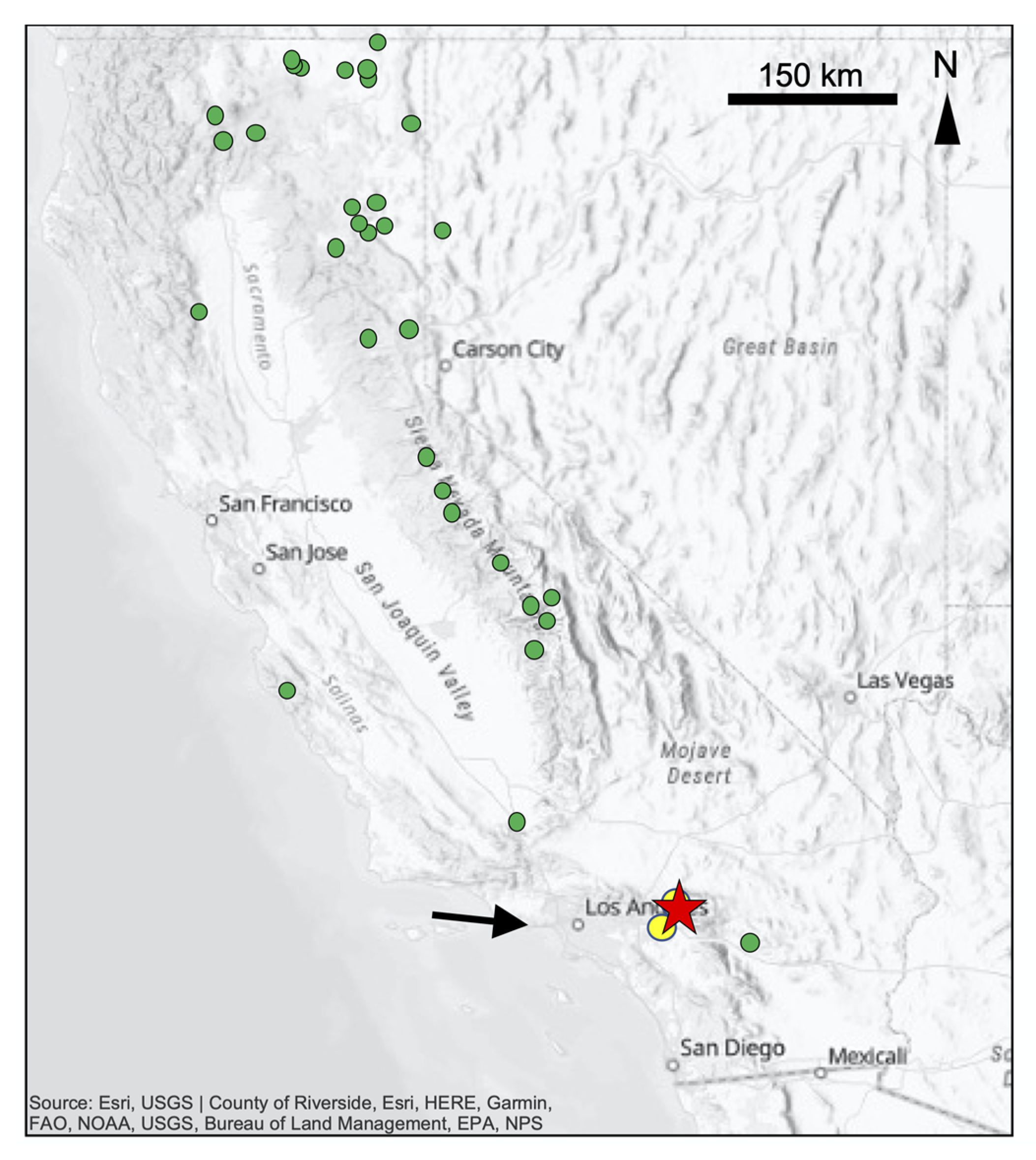
Increment cores were extracted from ponderosa pine trees located near Camp Seely in Crestline, CA (lat: 34.25° N, lon: 117.29° W) at an elevation of 1486 m above sea level (Figure 1). This location was chosen because it is on the west-facing slope of the San Bernardino Mountains and thus maximally exposed to the air pollution blowing eastward from Los Angeles, California. The forest is a mix-conifer forest characterized by Jeffrey (Pinus jeffreyi) and ponderosa pine (Pinus ponderosa) trees, sugar pine (Pinus lambertiana), incense cedar (Calocedrus decurrens), California black oak (Quercus kelloggii), and white fir (Abies concolor) [25]. However, in warmer dry environments like that of the San Bernardino Mountains, ponderosa pine often dominates the forest [37]. Thirty-four cores were extracted from 20 ponderosa pine trees near Camp Seely. All cores were taken at mean breast height (1.3 m above the land surface) in accordance with standard practice [38]. In total, 20 trees were sampled (2 cores per tree where possible) in accordance with standard dendrochronological techniques (Speer, 2010). In the case of 6 trees, only one core per tree was used; however, the expressed population signal (EPS) of the chronology indicated sufficient sampling depth and shared variability among trees was achieved to obtain a stand-level signal [39]. After extraction in the field, the cores were mounted and sanded to expose the transverse section and accentuate ring boundaries. Each core was placed on a Velmex tree ring measuring system (Velmex Inc. Bloomfield, NY, USA) and ring boundaries were cross-dated under a microscope and then measured to 0.001 mm. Once the ring widths for each core (radius) were compiled, the quality control program COFECHA [40] was used to verify the initial crossdating and detect regions of misalignment or low correlation between individual radii. The computer program ARSTAN [41,42] was used to compile individual ring-width series into a standardized chronology. This program removes non-climatic signals present in tree ring series including geometric and ecological growth trends resulting from intra-tree competition and local dynamics within the canopy. A cubic smoothing spline of 50% frequency response of 67% of the length of each series was used to standardize the series and an autoregressive model to remove autocorrelation effects was employed [43]. Statistics were computed on the chronology including interseries correlation, sensitivity, signal-to-noise ratio (SNR), autocorrelation, and the expressed population signal (EPS), which calculates how well a chronology represents the theoretical population [39].
2.2. Climate Data
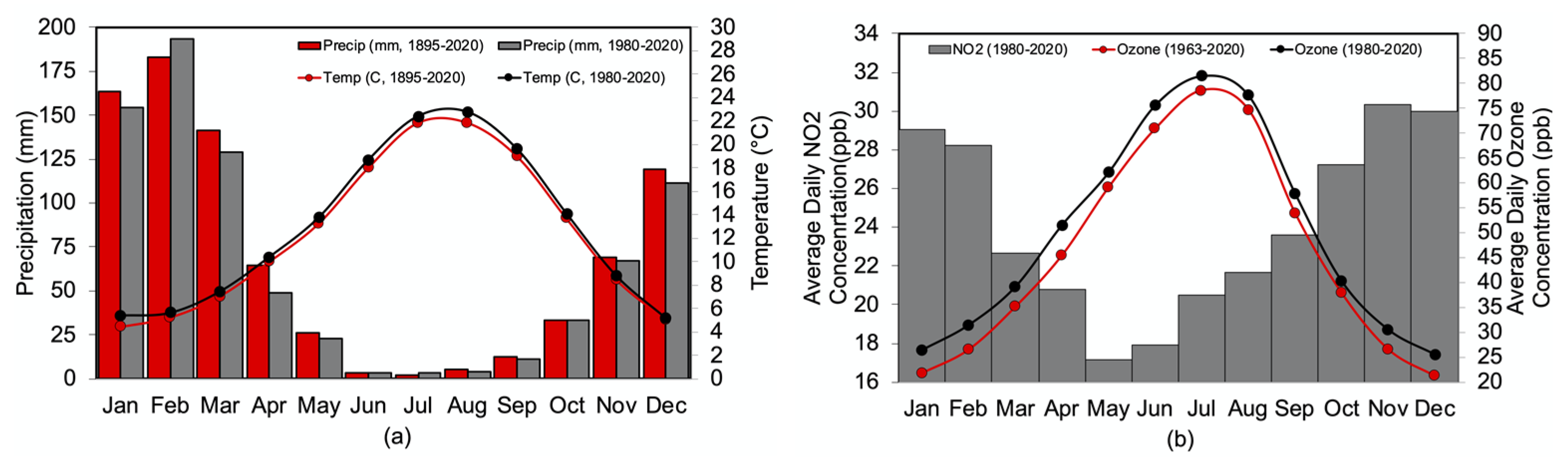
The site is characterized by a Mediterranean climate with wet winters and dry hot summers. In the San Bernardino mountains, the annual rainfall (824 mm) is less than half of that received in the Sierra Nevada (1778–2032 mm) and particularly deficient in the summer, where June–July–August–September total rainfall averages less than 25 mm. Thus, the trees in the study region experience seasonally limited water availability. The maximum rainfall occurs during the months of December through March while peak temperature occurs in July and August (Figure 2a). Total annual rainfall is 824 ± 1.6 mm and the average annual temperature is 12 ± 0.17 °C. Average maximum monthly temperature and total monthly precipitation data were obtained from the parameter-elevation regressions on independent slopes model (PRISM: https://prism.oregonstate.edu, [47]). The spatial resolution of this data is a 4-km2 grid-cell centered over the study site (lat: 34.25° N, lon: 117.29° W). PRISM temperature and precipitation data are available from 1895–2015 and were resolved into monthly, seasonal, and clusters of months to compare with the tree ring chronology. Several studies have assessed the reliability of PRISM data to accurately reproduce meteorological station data in southwestern United States [47] and specifically in mountainous regions such as the Transverse Ranges of California [48]. The Standardized Precipitation Evapotranspiration Index (SPEI, [49,50]) was also compared with the tree ring chronology. The SPEI includes both precipitation and evapotranspiration to capture the effect that temperature has on water demand. Data are available from 1901–2015 and calculated monthly at the site location (lat: 34.25° N, lon: 117.29° W) [51]. The Palmer Drought Severity Index (PDSI), a measure of the wetness and dryness of a region based on precipitation, moisture supply, runoff and evaporation, was also compared with the tree ring chronology. Data are spatially resolved at 2.5° × 2.5° (lat: 34.25° N, lon: 117.29° N) and are used from 1933–2015 in this study to overlap with the length of the tree ring chronology [52].
2.3. Air Pollution Data
In addition to the westward facing position of the study site that directly receives air pollution from Los Angeles, this site was also chosen because of the historical measurements of air pollution (ozone, O3) that have been recorded at Crestline since 1963 [53]. Hourly measurements of ozone have been made in this region since 1979 (lat: 33.99° N, lon: 117.41° W) and are available through the EPA’s Air Quality System database [46]. Measurements between 1963 and 1978 are reconstructed from episodic regional measurements from multiple sites, adjusting for differences in elevation, night-time concentration, and peak exposure [54]. Ozone data were resolved into monthly and seasonal composites over the time period and into clusters of months of peak maximum and minimum pollution values. Hourly measurements of nitrogen dioxide are also available through the EPA Air Quality System database [46] and were available over the time period 1980–2020 from the EPA station in Rubidoux, CA (lat: 34.00° N, lon: 117.24° W), although wintertime data (December–March) are missing between 2002–2006 and are not included in this study. Although pollution data are available through 2020, tree cores were extracted in 2015, which determines the final year of analysis. Average daily ozone concentration ranges from 21 ppb in the wet season to 79 ppb in the dry season (Figure 2b). Nitrogen dioxide shows an inverse relationship where peak values appear during the wet season (31.35 ppb in November) and diminish in the summer (18 ppb in May). However, month to month and year to year variability shows a positive correlation between O3 and NO2 (r = 0.88, p < 0.05) where a month (year) of high NO2 results in a month (year) of high levels of ozone and vice versa.
2.4. Climate Response Analysis
The relationship between climate variables and air pollution was examined by modeling the ability of 28 distinct combinations of monthly, seasonal, annual, and clustered grouped variables to predict the ring width chronology. Variables included total monthly precipitation, average monthly temperature, monthly SPEI, PDSI, average daily ozone (O3), and average daily nitrogen dioxide (NO2) from the previous October through the current year’s December. Wet season and dry season values were calculated along with the water year and other clustered months to examine relationships between tree growth and these variables. Multiple linear regressions were computed for all 28 time periods and t and p-values were calculated to determine statistical significance. A step-wise regression was employed to examine the relative importance of each variable to the overall tree ring signal. Variables with a variance inflation factor (VIF) greater than 3 were considered colinear and variables with a lower p-value were removed from the regression. A series of 5 separate step-wise regression models were compared.
3. Results
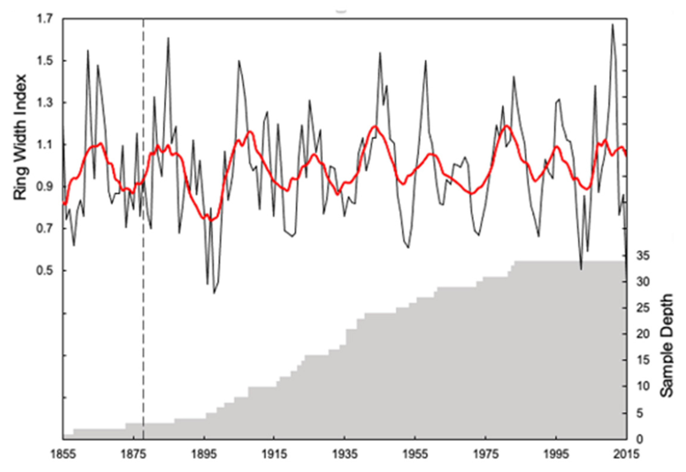
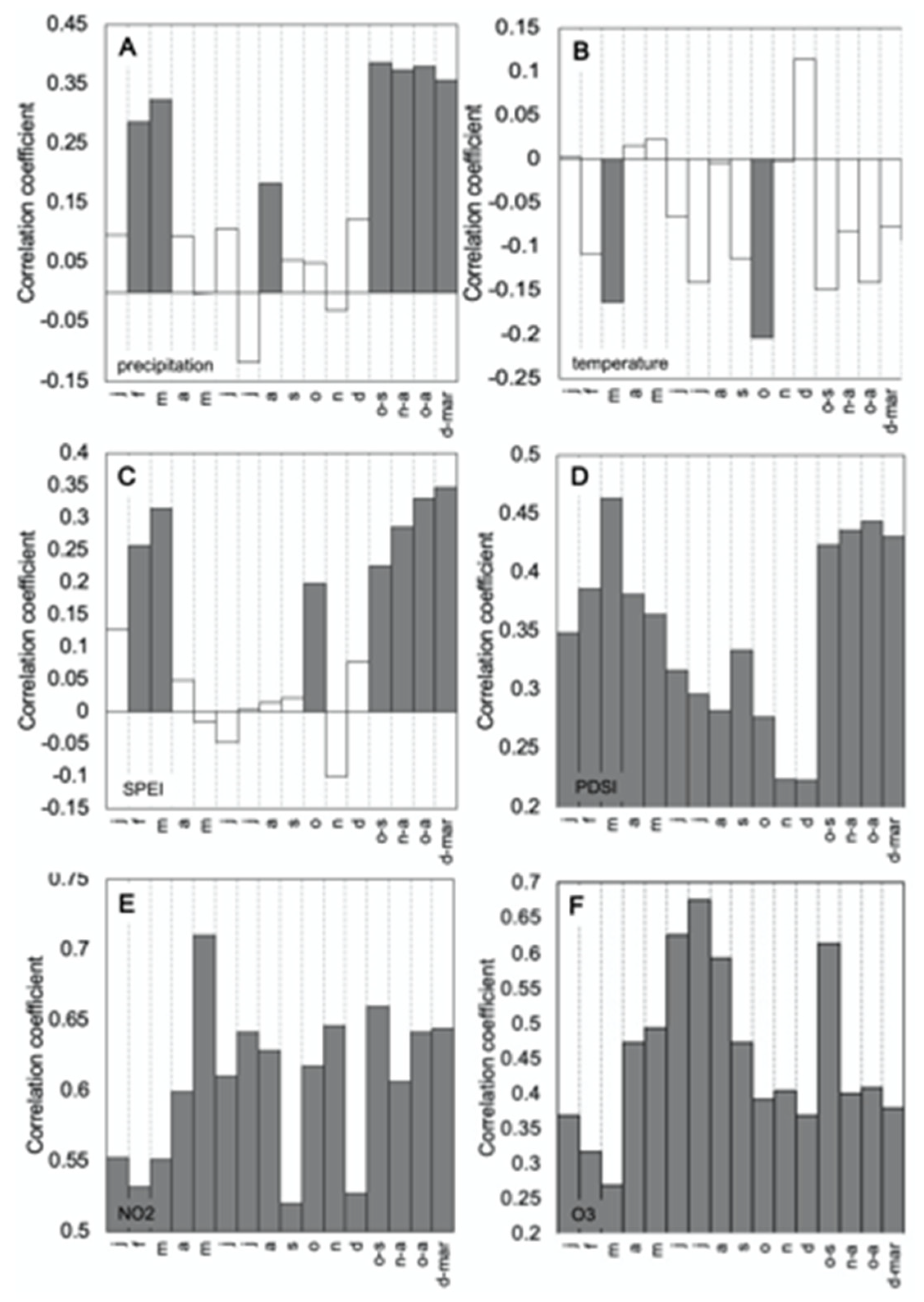
The Crestline ponderosa pine ring-width series crossdated well and showed good dendroclimatic potential, with the EPS of the site above the threshold limit of 0.85 for the standard chronology (Table 1). The running EPS shows the signal is robust from 1878 onward (Figure 3). The Signal to Noise (SNR) ratio is relatively high and the sensitivity is moderate (Table 1). When compared with precipitation, the tree ring chronology shows a statistically significant relationship with rainfall during the late part of the rainy season (February and March) and the month of August (Figure 4A, Table 2). However, the highest correlations were found between the tree ring chronology and the water year (pOct–Sep, r = 0.39, p < 0.05) and the previous wet season (pOct–Apr, r = 0.38, p < 0.05). Negative correlations were found between temperature and ponderosa pine growth, with the most significant correlation occurring between the tree chronology and temperature during the beginning of the previous rainy season (pOct, r = −0.27, p < 0.05) and the current rainy season (Oct, r = −0.20, p < 0.05) (Figure 4B, Table 2). A negative correlation was also found to be significant during the month of March of the current rainy season (r = −0.16, p < 0.05). Correlation between the SPEI and the tree chronology revealed a pattern similar to both precipitation and temperature, where statistically significant relationships were found during the start of the previous (pOct) and current rainy seasons (Oct), February, March, and the water year (pOct–Sep) (Figure 4C, Table 2). The highest correlation, however, was found between SPEI during the wet season (pDec–Mar, r = 0.35, p < 0.05). The chronology showed statistically significant (p < 0.05) correlation with PDSI during all monthly, seasonal, and clustered time periods examined, with the strongest correlations occurring during the month of March (r = 0.46, p < 0.05) and during the rainy season (pOct–Apr, r = 0.44, p < 0.05) (Figure 4D, Table 2). The highest climate forcing correlations overall were found between the tree chronology and PDSI, although the next strongest correlations were found between the tree chronology and precipitation (Table 2, Supplementary Figure S1).
Monthly average NO2 concentrations were found to be well correlated with tree growth during all months examined, including seasonal clusters (wet season, dry season), and the water year (Figure 4E). The highest correlation is found between the chronology and May NO2 concentrations (r = 0.71, p < 0.05) and the water year (pOct–Sep, r = 0.66, p < 0.05). Ozone is also positively correlated with tree growth, particularly when ozone levels peak during the dry season (Jun–Aug, r = 0.67, p < 0.05); however, this is to be expected given that NO2 and O3 are strongly correlated (r = 0.84, p < 0.05) (Figure 4F).
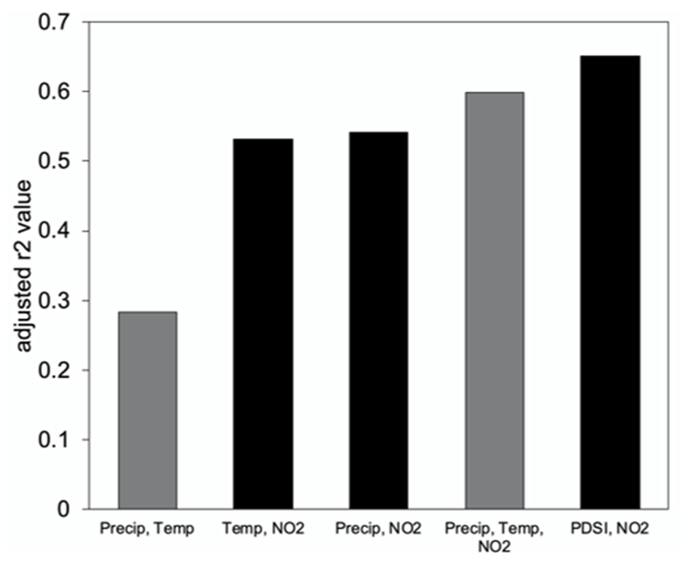
A stepwise multiple linear regression showed that the most important driver of ring-width increment is NO2 during the water year (pOct–Sep), which is also observed in the individually computed correlations (Table 3). PDSI during March is also a significant driver of growth and, with NO2 (pOct–Sep), explains a significant component of tree ring growth variability (r2-adj = 0.65, p < 0.001). Combinations of precipitation (pOct–Sep), temperature (pOct), NO2 (pOct–Sep), and PDSI (March) can be used to represent tree ring variability in several step-wise regression models (Figure 5). Precipitation is found to be the primary driver of ring-width increment size when only precipitation and temperature are used (Figure 5). However, when NO2 is introduced, the model results in a far more significant adjusted r2 value (Figure 5). PDSI and precipitation as well as PDSI and temperature were found to covary (VIF > 3) and, thus, are not included together in any stepwise regression model. Similarly, ozone and nitrogen dioxide were found to covary (VIF = 3.4) and are not included together in any model for the same reason. The models that yielded the highest adjusted r2 values and, thus, best represented the tree ring chronology were PDSI and NO2 (r2-adj = 0.65, p < 0.001) and temperature, precipitation, and NO2 (r2-adj = 0.60, p < 0.05). Using the PDSI (Mar) and NO2 (pOct–Sep) to reconstruct the tree ring chronology yields the strongest correlation (r2 = 0.671) (Figure 6). The individual climate response analyses and the stepwise multiple regressions indicate that drought conditions (PDSI) at the end of the rainy season (March) and NO2 pollution during the growing year (pOct–Sep) exhibit primary controls on growth for ponderosa pine growing in this region.
4. Discussion
4.1. Climate and Tree Increment Growth
Variations in ring width of the ponderosa pine trees from the Crestline region are driven by precipitation and temperature. In general, the climate sensitivity of this chronology to temperature, precipitation, and drought indices is consistent with that found in other studies of Ponderosa pine trees in the southwestern United States [1,55,56,57]. Rainfall during the growing season has been found to drive growth in ponderosa pine trees growing in the Rocky Mountains [56] and in the Sierra Nevada [58]. McCullough et al. [1] found that wet season precipitation is one of the main drivers of growth across both Pacific interior and coastal forests of ponderosa pine, although trees in the southwest and coast ranges were found to be less sensitive to climate than those located more inland. Their findings are supported by this study, where sensitivity to water year precipitation is statistically significant, but lower than expected (Table 1). Temperature has some control over the tree ring signal, where higher temperatures during the onset of the rainy season (pOct) are associated with lower amounts of basal increment growth (Figure 4B). Combining temperature and precipitation into a moisture availability index (SPEI) yields a statistically significant relationship with tree growth as well, suggesting that both temperature and precipitation during the wet season determine the growth of the tree bole (Figure 5). However, the strongest climate determinant of tree growth appears to be moisture availability as represented in the PDSI, which incorporates water demand, moisture availability, temperature, and precipitation (Table 2). As precipitation decreases and temperature increases, this generates higher water demand, which enhances drought severity and reduces increment growth in ponderosa pine trees in this region. While the stepwise multiple regression reveals that the tree ring chronology can be explained by water year precipitation and rainy season temperature, a much greater portion of the variability is explained when an integrated drought index (PDSI) is used, owing to the interplay between water demand and drought and the ability of this index to retain the memory of previous (9–19 months) climate conditions (Figure 5) [59]. A more integrated representation of climate conditions yields a higher correlation with tree growth given that tree radial increments are annual.
4.2. NO2, Ozone, and Tree Growth
Previous studies have discovered a connection between bole growth and increasing N deposition, even in the presence of elevated ozone, which is phytotoxic [60]. In 2020, Fenn et al. [32] measured changes in aboveground biomass in the San Bernardino National Forest over a 10-year period using Forest Inventory and Analysis (FIA) plots. Their findings showed increases in carbon increment across a range of species in response to N deposition. Notably, regions with high levels of both ozone and N deposition still showed a positive increase in carbon increment, needle growth, and aboveground woody biomass [32]. The findings of this study corroborate this assessment, showing that NO2 concentrations and tree ring width covary significantly. Grulke et al. [61] explain that a nitrogen-driven increase in aboveground biomass may occur at the expense of fine and coarse root growth. This effect is not linear, however, given that moderate exposure to ozone (20–30 ppb) and N deposition (15–25 kg ha−1 yr−1) resulted in diminished carbon increment (CI) for ponderosa pine [32]. This may explain why prior studies [62,63] observed diminished growth in response to elevated ozone levels in this region. However, the increased growth in response to elevated NO2 and ozone in this study may be explained by the extremely high levels of pollution in this region (Figure 4) [64]. The average ozone levels for this study site are much higher (annual average = 50.3 ppb) and, therefore, result in an increase in the allocation of aboveground biomass as observed in the increased ring widths in the trees growing at Crestline. Increased CI growth in response to ozone and N deposition is expected when the ozone levels are sufficiently high (>30 ppb) as confirmed by other studies [32,60].
Nitrogen dioxide emissions throughout the growing season strongly correlate with tree growth and explain the majority (r2 = 0.50, p < 0.05) of the tree ring signals (Figure 5). Because N deposition enhances growth in this region, it may be observed to counter the negative impacts of ozone exposure, by increasing growth in the bole of the tree and enhancing N availability for photosynthetic pigment repair [65]. However, Grulke [26] observed an increase in stomatal conductance and ozone uptake in response to increased N availability, suggesting that trees may experience greater drought stress amid high levels of pollutants, thus enhancing their sensitivity to climate. One way to test this would be to contrast the sensitivity of tree growth to climate before and after the influence of air pollution in the study region, because it is not possible to disentangle the relative contributions of pollution and climate over the common period (1980–2015). However, this requires a longer time series of pollution data over the length of the tree chronology (1855–2015), which is not available. Nevertheless, the variables that best explain the variability in tree ring growth include both moisture availability (PDSI) and nitrogen dioxide, which seem to support this idea (Figure 5).
One possible hypothesis for the increased growth observed during high nitrogen dioxide years relates to the interplay between precipitation and N deposition, given that arid conditions can reduce N retention and uptake by needles [66,67]. Because the canopy can retain N via dry deposition [68], this stored N may be flushed to the rooting zone during high rainfall events or high rainfall months. One possible explanation, therefore, may be that rainfall events at the end of the rainy season (March–May) flush N to the rooting zone where it is available for uptake. It is also possible that the milder winter conditions of the Transverse Ranges and the mid-elevation of the study site facilitate the biological availability and assimilation of N during spring rainfall events [32].
4.3. Colinearity of Ozone and Nitrogen Dioxide
Although a direct link between ozone exposure alone and increased radial increment growth has not been found previously, a correlation between peak ozone emission (July, 79 ppb) and tree growth is observed in this study (Figure 4F). This is likely related to the co-occurrence of N deposition via nitrous oxides and ozone, as observed in this region (r2 = 0.71, p < 0.05). As previously mentioned, high levels of ozone and N deposition in combination have been found to stimulate bole growth in ponderosa pine trees in California and this study corroborates this finding [32]. However, because ozone is phytotoxic and has been shown to result in premature needle loss [27], diminished crown capacity, and reduced stomatal conductance [61], using this variable to explain variability in the radial increment of ponderosa pine growth may not be entirely appropriate. Additionally, the covariability of ozone and nitrogen dioxide generated a VIF greater than 3 (VIF = 3.4), which precluded its use in the stepwise multiple regression. Nevertheless, the diffuse impacts of ozone and N deposition can be observed to have significant control over radial growth variability in ponderosa pine trees in a heavily polluted region [69]. Nitrogen dioxide emissions, when combined with moisture availability (PDSI) explain 67.1% (p < 0.01) of the variability in incremental tree growth in the ponderosa pine trees growing at Crestline, CA (Figure 5). One important question that emerges from this work concerns how ponderosa pine trees in the San Bernardino forest will respond to increasingly high levels of nitrogen, ozone, and increasing temperature in the future, particularly in contrast with those growing in the Sierra Nevada.
5. Conclusions
Ponderosa pine tree rings at the Crestline site cross-dated well and showed a statistically significant correlation with water year and rainy season precipitation and rainy season temperature. The strongest climatic relationships are found between the tree ring chronology and moisture availability during the water year (PDSI). Year to year variability in tree growth can be explained by variations in nitrogen dioxide and ozone concentration in this heavily polluted region, particularly during the water year (NO2) and the dry season (ozone). This suggests that trees in this region show increased increment (bole) growth in response to high (>30 ppb) levels of ozone pollution and N deposition, likely associated with changes in above and belowground carbon allocation in response to stress. Together, an integrated measure of moisture availability and nitrogen dioxide pollution explain 67.1% (p < 0.01) of the variability of the tree ring growth signal, suggesting trees in this region are strongly affected by external stressors of climate and air pollution.
Supplementary Materials
The following are available online at https://www.mdpi.com/article/10.3390/cli9050082/s1, Figure S1: Stacked Time Series plots of selected datasets examined in this study including (from top to bottom) the Crestline Tree Ring Chronology (this study), Total Water Year Precipitation (Oct-Sep), Average Dec-Mar Standardized Precipitation and Evapotranspiration Index (SPEI), Average October Temperature, Average March Palmer Drought Severity Index (PDSI), Average Daily Concentration of Ozone during the month of July, Average Daily Concentration of Nitrogen Dioxide (NO2) during the month of May. Time periods are selected based on statistically significant (p < 0.05) correlation with the tree ring chronology as reported in Table 2 and Figure 4. Precipitation and Temperature data obtained from the Parameter-elevation regressions on independent slopes model (PRISM, [31]) from 1895–2015. Standardized Precipitation Evapotranspiration Index (SPEI, [32,33]) available over the study site from 1901–2015. Palmer Drought Severity Index Data [35] are spatially resolved at 2.5° × 2.5° (lat: 34.25° N, lon: 117.25° N) and are used from 1933–2015. Ozone and Nitrogen Dioxide data available from EPA’s Air Quality System database [50] from 1963–2020 and 1980–2020 (data missing from 2002–2006), respectively.
Funding
This research was funded by the University of Redlands through Faculty Start-Up Funds, a University of Redlands Faculty Research Grant, and the University of Redlands Summer Science Research Program Endowment.
Data Availability Statement
The data presented in this study is openly available in the International Tree Ring Database (ITRDB) and also available from the author upon request.
Acknowledgments
I gratefully acknowledge the University of Redlands Center for Spatial Studies, Blodwyn McIntyre for her field labor, Scout Dahms-May for her field labor and laboratory processing, and the San Bernardino National Forest Service for allowing this research to take place on forest land.
Conflicts of Interest
The authors declare no conflict of interest. The funders had no role in the design of the study; in the collection, analyses, or interpretation of data; in the writing of the manuscript, or in the decision to publish the results.
References
- McCullough, I.M.; Davis, F.W.; Williams, A.P. A range of possibilities: Assessing geographic variation in climate sensitivity of ponderosa pine using tree rings. For. Ecol. Manag. 2017, 402, 223–233. [Google Scholar] [CrossRef]
- Graumlich, L.J. A 1000-Year Record of Temperature and Precipitation in the Sierra Nevada. Quat. Res. 1993, 39, 249–255. [Google Scholar] [CrossRef]
- Kerhoulas, L.P.; Kolb, T.E.; Koch, G.W. The Influence of Monsoon Climate on Latewood Growth of Southwestern Ponderosa Pine. Forests 2017, 8, 140. [Google Scholar] [CrossRef] [Green Version]
- Dannenberg, M.P.; Wise, E.K. Seasonal climate signals from multiple tree ring metrics: A case study of Pinus ponderosa in the upper Columbia River Basin. J. Geophys. Res. Biogeosci. 2016, 121, 1178–1189. [Google Scholar] [CrossRef] [Green Version]
- Kerhoulas, L.P.; Kane, J.M. Sensitivity of ring growth and carbon allocation to climatic variation vary within ponderosa pine trees. Tree Physiol. 2011, 32, 14–23. [Google Scholar] [CrossRef] [PubMed] [Green Version]
- Salzer, M.W.; Kipfmueller, K.F. Reconstructed Temperature and Precipitation on A Millennial Timescale from Tree-Rings in the Southern Colorado Plateau, U.S.A. Clim. Chang. 2005, 70, 465–487. [Google Scholar] [CrossRef]
- Fuchs, L.; Stevens, L.E.; Fulé, P.Z. Dendrochronological assessment of springs effects on ponderosa pine growth, Arizona, USA. For. Ecol. Manag. 2019, 435, 89–96. [Google Scholar] [CrossRef]
- Brown, P.M.; Wu, R. Climate and disturbance forcing of episodic tree recruitment in a southwestern ponderosa pine landscape. Ecology 2005, 86, 3030–3038. [Google Scholar] [CrossRef]
- Leavitt, S.W.; Wright, W.E.; Long, A. Spatial expression of ENSO, drought, and summer monsoon in seasonal δ13C of ponderosa pine tree rings in southern Arizona and New Mexico. J. Geophys. Res. Space Phys. 2002, 107. [Google Scholar] [CrossRef]
- Cook, E.R.; Woodhouse, C.A.; Eakin, C.M.; Meko, D.M.; Stahle, D.W. Long-Term Aridity Changes in the Western United States. Science 2004, 306, 1015–1018. [Google Scholar] [CrossRef] [Green Version]
- Stephens, S.L.; Lydersen, J.M.; Collins, B.M.; Fry, D.L.; Meyer, M.D. Historical and current landscape-scale ponderosa pine and mixed conifer forest structure in the Southern Sierra Nevada. Ecosphere 2015, 6, art79. [Google Scholar] [CrossRef]
- Koppen, W. Das geographische system der klimat. Handb. Klimatol. 1936, 46, 1–44. [Google Scholar]
- Rosenthal, J.S.; Helvey, R.A.; Battalino, T.E.; Fisk, C.; Greiman, P.W. Ozone transport by mesoscale and diurnal wind circulations across southern California. Atmos. Environ. 2003, 37, 51–71. [Google Scholar] [CrossRef]
- Miller, P.R.; Taylor, O.C.; McBride, J.R. Oxidant Air Pollution Impacts in the Montane Forests of Southern California: A Case Study of the San Bernardino Mountains; Springer: New York, NY, USA, 2012. [Google Scholar]
- Bao, J.-W.; Michelson, S.A.; Persson, P.O.G.; Djalalova, I.V.; Wilczak, J.M. Observed and WRF-Simulated Low-Level Winds in a High-Ozone Episode during the Central California Ozone Study. J. Appl. Meteorol. Clim. 2008, 47, 2372–2394. [Google Scholar] [CrossRef]
- Parrish, D.D.; Xu, J.; Croes, B.; Shao, M. Air quality improvement in Los Angeles—Perspectives for developing cities. Front. Environ. Sci. Eng. 2016, 10, 11. [Google Scholar] [CrossRef]
- Docherty, K.S.; Aiken, A.C.; Huffman, J.A.; Ulbrich, I.M.; Decarlo, P.F.; Sueper, D.; Worsnop, D.R.; Snyder, D.C.; Peltier, R.E.; Weber, R.J.; et al. The 2005 Study of Organic Aerosols at Riverside (SOAR-1): Instrumental intercomparisons and fine particle composition. Atmos. Chem. Phys. Discuss. 2011, 11, 12387–12420. [Google Scholar] [CrossRef] [Green Version]
- Ryerson, T.B.; Andrews, A.E.; Angevine, W.M.; Bates, T.S.; Brock, C.A.; Cairns, B.; Cohen, R.C.; Cooper, O.R.; De Gouw, J.A.; Fehsenfeld, F.C.; et al. The 2010 California Research at the Nexus of Air Quality and Climate Change (CalNex) field study. J. Geophys. Res. Atmos. 2013, 118, 5830–5866. [Google Scholar] [CrossRef]
- Park, C.; Gerbig, C.; Newman, S.; Ahmadov, R.; Feng, S.; Gurney, K.R.; Carmichael, G.R.; Park, S.-Y.; Lee, H.-W.; Goulden, M.; et al. CO2 Transport, Variability, and Budget over the Southern California Air Basin Using the High-Resolution WRF-VPRM Model during the CalNex 2010 Campaign. J. Appl. Meteorol. Clim. 2018, 57, 1337–1352. [Google Scholar] [CrossRef]
- Trouet, V.; Taylor, A.H.; Wahl, E.R.; Skinner, C.N.; Stephens, S.L. Fire-climate interactions in the American West since 1400 CE. Geophys. Res. Lett. 2010, 37. [Google Scholar] [CrossRef] [Green Version]
- Steiner, A.L.; Tonse, S.; Cohen, R.C.; Goldstein, A.H.; Harley, R.A. Influence of future climate and emissions on regional air quality in California. J. Geophys. Res. Space Phys. 2006, 111. [Google Scholar] [CrossRef]
- Johnson, C.E.; Collins, W.J.; Stevenson, D.S.; Derwent, R.G. Relative roles of climate and emissions changes on future tropospheric oxidant concentrations. J. Geophys. Res. Space Phys. 1999, 104, 18631–18645. [Google Scholar] [CrossRef] [Green Version]
- Mickley, L.J.; Jacob, D.J.; Field, B.D.; Rind, D. Effects of future climate change on regional air pollution episodes in the United States. Geophys. Res. Lett. 2004, 31. [Google Scholar] [CrossRef]
- Leung, L.R.; Gustafson, W.I., Jr. Potential regional climate change and implications to US air quality. Geophys. Res. Lett. 2005, 32, L16711. [Google Scholar] [CrossRef] [Green Version]
- Arbaugh, M.J.; Peterson, D.L.; Miller, P.R. Air Pollution Effects on Growth of Ponderosa Pine, Jeffrey Pine, and Bigcone Douglas-Fir. In Oxidant Air Pollution Impacts in the Montane Forests of Southern California: A Case Study of the San Bernardino Mountains; Miller, P.R., McBride, J.R., Eds.; Springer: New York, NY, USA, 1999; pp. 179–207. [Google Scholar]
- Grulke, N.E. The Physiological Basis of Ozone Injury Assessment Attributes in Sierran Conifers. In Developments in Environmental Science; Elsevier Science Ltd.: Amsterdam, The Netherlands, 2003; Chapter 3; Volume 2, pp. 55–81. [Google Scholar]
- Evans, L.S.; Miller, P.R. Histological Comparison of Single and Additive O3 and SO2 Injuries to Elongating Ponderosa Pine Needles. Am. J. Bot. 1975, 62, 416. [Google Scholar] [CrossRef]
- Tingey, D.T.; Hogsett, W.E.; Lee, E.H.; Laurence, J.A. Stricter Ozone Ambient Air Quality Standard Has Beneficial Effect on Ponderosa Pine in California. Environ. Manag. 2004, 34, 397–405. [Google Scholar] [CrossRef] [PubMed]
- Agathokleous, E.; Saitanis, C.J.; Wang, X.; Watanabe, M.; Koike, T. A Review Study on Past 40 Years of Research on Effects of Tropospheric O3 on Belowground Structure, Functioning, and Processes of Trees: A Linkage with Potential Ecological Implications. Water, Air, Soil Pollut. 2015, 227, 1–28. [Google Scholar] [CrossRef]
- Mills, G.; Harmens, H.; Wagg, S.; Sharps, K.; Hayes, F.; Fowler, D.; Sutton, M.; Davies, B. Ozone impacts on vegetation in a nitrogen enriched and changing climate. Environ. Pollut. 2016, 208, 898–908. [Google Scholar] [CrossRef] [Green Version]
- Grulke, N.; Andersen, C.; Fenn, M.; Miller, P. Ozone exposure and nitrogen deposition lowers root biomass of ponderosa pine in the San Bernardino Mountains, California. Environ. Pollut. 1998, 103, 63–73. [Google Scholar] [CrossRef]
- Fenn, M.E.; Preisler, H.K.; Fried, J.S.; Bytnerowicz, A.; Schilling, S.L.; Jovan, S.; Kuegler, O. Evaluating the effects of nitrogen and sulfur deposition and ozone on tree growth and mortality in California using a spatially comprehensive forest inventory. For. Ecol. Manag. 2020, 465, 118084. [Google Scholar] [CrossRef]
- Grulke, N.E.; Heath, R.L. Ozone effects on plants in natural ecosystems. Plant Biol. 2019, 22, 12–37. [Google Scholar] [CrossRef]
- Negrón, J.F.; McMillin, J.D.; Anhold, J.A.; Coulson, D. Bark beetle-caused mortality in a drought-affected ponderosa pine landscape in Arizona, USA. For. Ecol. Manag. 2009, 257, 1353–1362. [Google Scholar] [CrossRef]
- Ferretti, M.; Bacaro, G.; Brunialti, G.; Confalonieri, M.; Cristofolini, F.; Cristofori, A.; Frati, L.; Finco, A.; Gerosa, G.; Maccherini, S.; et al. Scarce evidence of ozone effect on recent health and productivity of alpine forests—A case study in Trentino, N. Italy. Environ. Sci. Pollut. Res. 2018, 25, 8217–8232. [Google Scholar] [CrossRef]
- Grulke, N.E.; Minnich, R.A.; Paine, T.D.; Seybold, S.J.; Chavez, D.J.; Fenn, M.E.; Riggan, P.J.; Dunn, A. Chapter 17 Air Pollution Increases Forest Susceptibility to Wildfires: A Case Study in the San Bernardino Mountains in Southern California. Wildland Fires Air Pollut. 2009, 8, 365. [Google Scholar] [CrossRef]
- Griffin, J.R. The Distribution of Forest Trees in California; Pacific Southwest Forest and Range Experiment Station: Berkeley, CA USA, 1972; Volume 82. [Google Scholar]
- Speer, J.H. Fundamentals of Tree-Ring Research; University of Arizona Press: Tucson, AZ, USA, 2010. [Google Scholar]
- Wigley, T.M.L.; Briffa, K.R.; Jones, P.D. On the Average Value of Correlated Time Series, with Applications in Den-droclimatology and Hydrometeorology. J. Appl. Meteorol. Climatol. 1984, 23, 201–213. [Google Scholar] [CrossRef]
- Holmes, R. Computer-Assisted Quality Control in Tree-Ring Dating and Measurement. Tree-Ring Bull. 1983, 43, 51–67. [Google Scholar]
- LDEO. ARSTAN; Lamont-Doherty Earth Observatory: New York, NY, USA, 2014. [Google Scholar]
- Cook, E.R. A Time Series Analysis Approach to Tree-Ring Standardization; University of Arizona: Tucson, AZ, USA, 1985; 171p. [Google Scholar]
- Cook, E.R. The Decomposition of Tree-Ring Series for Environmental Studies; Tree-Ring Bulletin: Tree Ring Society: Tucson, AZ, USA, 1987; Volume 47, pp. 37–59. [Google Scholar]
- Edinger, J.G.; McCutchan, M.H.; Miller, P.R.; Ryan, B.C.; Schroeder, M.J.; Behar, J.V. Penetration and Duration of Oxidant Air Pollution in the South Coast Air Basin of California. J. Air Pollut. Control. Assoc. 1972, 22, 882–886. [Google Scholar] [CrossRef]
- Winant, C.D.; Dorman, C.E. Seasonal patterns of surface wind stress and heat flux over the Southern California Bight. J. Geophys. Res. Space Phys. 1997, 102, 5641–5653. [Google Scholar] [CrossRef]
- US Environmental Protection Agency. Air Quality System Data Mart. 2021. Available online: https://www.epa.gov/airdata (accessed on 15 January 2021).
- Daly, C.; Halbleib, M.; Smith, J.I.; Gibson, W.P.; Doggett, M.K.; Taylor, G.H.; Curtis, J.; Pasteris, P.P. Physiographically sensitive mapping of climatological temperature and precipitation across the conterminous United States. Int. J. Clim. 2008, 28, 2031–2064. [Google Scholar] [CrossRef]
- Strachan, S.; Daly, C. Testing the daily PRISM air temperature model on semiarid mountain slopes. J. Geophys. Res. Atmos. 2017, 122, 5697–5715. [Google Scholar] [CrossRef]
- Beguería, S.; Vicente-Serrano, S.M.; Reig-Gracia, F.; Latorre, B. Standardized precipitation evapotranspiration index (SPEI) revisited: Parameter fitting, evapotranspiration models, tools, datasets and drought monitoring. Int. J. Clim. 2014, 34, 3001–3023. [Google Scholar] [CrossRef] [Green Version]
- Beguería, S.; Vicente-Serrano, S.M.; Angulo-Martínez, M. A Multiscalar Global Drought Dataset: The SPEIbase: A New Gridded Product for the Analysis of Drought Variability and Impacts. Bull. Am. Meteorol. Soc. 2010, 91, 1351–1356. [Google Scholar] [CrossRef] [Green Version]
- Vicente-Serrano, S.M.; Beguería, S.; López-Moreno, J.I.; Angulo, M.; El Kenawy, A. A New Global 0.5° Gridded Dataset (1901–2006) of a Multiscalar Drought Index: Comparison with Current Drought Index Datasets Based on the Palmer Drought Severity Index. J. Hydrometeorol. 2010, 11, 1033–1043. [Google Scholar] [CrossRef] [Green Version]
- Zhao, T.; Dai, A. The Magnitude and Causes of Global Drought Changes in the Twenty-First Century under a Low–Moderate Emissions Scenario. J. Clim. 2015, 28, 4490–4512. [Google Scholar] [CrossRef]
- Lee, E.; Tingey, D.T.; Hogsett, W.E.; Laurence, J.A. History of tropospheric ozone for the San Bernardino Mountains of Southern California, 1963–1999. Atmos. Environ. 2003, 37, 2705–2717. [Google Scholar] [CrossRef]
- Lee, E. Use of auxiliary data for spatial interpolation of surface ozone patterns. In Developments in Environmental Science; Elsevier: Amsterdam, The Netherlands, 2003; pp. 165–194. [Google Scholar]
- Finley, K.; Zhang, J. Climate Effect on Ponderosa Pine Radial Growth Varies with Tree Density and Shrub Removal. Forests 2019, 10, 477. [Google Scholar] [CrossRef] [Green Version]
- Pettit, J.L.; Derose, R.J.; Long, J.N. Climatic Drivers of Ponderosa Pine Growth in Central Idaho. Tree-Ring Res. 2018, 74, 172–184. [Google Scholar] [CrossRef]
- Peltier, D.M.P.; Ogle, K. Legacies of more frequent drought in ponderosa pine across the western United States. Glob. Chang. Biol. 2019, 25, 3803–3816. [Google Scholar] [CrossRef]
- Shamir, E.; Meko, D.; Touchan, R.; Lepley, K.S.; Campbell, R.; Kaliff, R.N.; Georgakakos, K.P. Snowpack- and Soil Water Content-Related Hydrologic Indices and Their Association With Radial Growth of Conifers in the Sierra Nevada, California. J. Geophys. Res. Biogeosci. 2020, 125. [Google Scholar] [CrossRef]
- Zhao, H.; Gao, G.; An, W.; Zou, X.; Li, H.; Hou, M. Timescale differences between SC-PDSI and SPEI for drought monitoring in China. Phys. Chem. Earth Parts ABC 2017, 102, 48–58. [Google Scholar] [CrossRef]
- Grulke, N.; Balduman, L. Deciduous Conifers: High N Deposition and O3 Exposure Effects on Growth and Biomass Allocation in Ponderosa Pine. Water, Air, Soil Pollut. 1999, 116, 235–248. [Google Scholar] [CrossRef]
- Grulke, N.E. Physiological Responses of Ponderosa Pine to Gradients of Environmental Stressors. In Oxidant Air Pollution Impacts in the Montane Forests of Southern California: A Case Study of the San Bernardino Mountains; Miller, P.R., McBride, J.R., Eds.; Springer: New York, NY, USA, 1999; pp. 126–163. [Google Scholar]
- Miller, P.R.; Arbaugh, M.J.; Temple, P.J. Ozone and Its Known and Potential Effects on Forests in Western United States. In Forest Decline and Ozone: A Comparison of Controlled Chamber and Field Experiments; Sandermann, H., Wellburn, A.R., Heath, R.L., Eds.; Springer: Berlin/Heidelberg, Germany, 1997; pp. 39–67. [Google Scholar]
- Miller, P.R.; Longbotham, G.J.; Longbotham, C. Sensitivity of selected western conifers to ozone. Plant Dis. 1983, 67, 1113–1115. [Google Scholar] [CrossRef]
- Lorenz, M.; Clarke, N.; Paoletti, E.; Bytnerowicz, A.; Grulke, N.; Lukina, N.; Sase, H.; Staelens, J. Air Pollution Impacts on Forests in a Changing Climate; International Union of Forest Research Organizations (IUFRO): Vienna, Austria, 2010. [Google Scholar]
- Beyers, J.L.; Riechers, G.H.; Temple, P.J. Effects of long-term ozone exposure and drought on the photosynthetic capacity of ponderosa pine (Pinus ponderosa Laws). New Phytol. 1992, 122, 81–90. [Google Scholar] [CrossRef] [PubMed]
- Padgett, P. Nitrogen deposition: The up and down side for production and down side for production agriculture. Plant Physiol. 2009, 101, 141–146. [Google Scholar] [CrossRef] [PubMed] [Green Version]
- Temple, P.J.; Miller, P.R. Seasonal influences on ozone uptake and foliar injury to ponderosa and Jeffrey pines at a southern California site. In Proceedings of the International Symposium on Air Pollution and Climate Change Effects on Forest Ecosystems, Albany, CA, USA, 5–9 February 1996; pp. 221–228. [Google Scholar]
- Avila, A.; Aguillaume, L.; Izquieta-Rojano, S.; García-Gómez, H.; Elustondo, D.; Santamaría, J.M.; Alonso, R. Quantitative study on nitrogen deposition and canopy retention in Mediterranean evergreen forests. Environ. Sci. Pollut. Res. 2017, 24, 26213–26226. [Google Scholar] [CrossRef] [PubMed] [Green Version]
- Paoletti, E.; Bytnerowicz, A.; Andersen, C.; Augustaitis, A.; Ferretti, M.; Grulke, N.; Günthardt-Goerg, M.S.; Innes, J.; Johnson, D.; Karnosky, D.; et al. Impacts of Air Pollution and Climate Change on Forest Ecosystems—Emerging Research Needs. Sci. World J. 2007, 7, 1–8. [Google Scholar] [CrossRef]
Figure 1.
Map showing the location of the Crestline ponderosa pine chronology used in this study (red star). Green circles represent the locations of existing ITRDB ponderosa pine chronologies, available at https://www.ncdc.noaa.gov/data-access/paleoclimatology-data. Black arrow denotes the dominant wind direction over the study site [44,45] and yellow circles locate the sites of NO2 (southern circle), and ozone (northern circle) air pollution measurements [46].

Figure 2.
Climatology and pollution over the studied period (a) is the mean climatology over the study site calculated over the length of the time series (1895–2020) and calculated over the common period (1980–2020). Precipitation (1895–2020) given in red bars, precipitation (1980–2020) given in gray bars. Temperature (1895–2020) given in the red line, temperature (1980–2020) given in the black line. Data from PRISM, Spatial resolution 4km2, Lat: 34.25° N, Lon: 117.29° N [47]. (b) is the average daily concentrations of O3 per month over the length of the time series (1963–2020) given in the red line and over the common period (1980–2020) given in the black line and NO2 per month (1980–2020) given in the gray bars at the study site. Data from EPA AIRS [46].

Figure 3.
Tree ring chronology for the Crestline ponderosa pine. A 10-year running mean is plotted in red and the number of tree samples used is shaded in gray. The point at which the chronology exceeds an expressed population (EPS) threshold of 0.85 is given by the dashed line.
Figure 3.
Tree ring chronology for the Crestline ponderosa pine. A 10-year running mean is plotted in red and the number of tree samples used is shaded in gray. The point at which the chronology exceeds an expressed population (EPS) threshold of 0.85 is given by the dashed line.

Figure 4.
Relationships between the Crestline tree ring chronology and selected months and seasons for (A) total precipitation (1895–2015), (B) average temperature (1895–2015), (C) average SPEI (1901–2015), (D) average PDSI (1933–2015), (E) daily average NO2 concentration (1980–2015), and (F) daily average O3 concentration (1963–2015).

Figure 5.
Adjusted r2 values produced by different stepwise regression models. Variables included in the models were precipitation (pOct–Sep), temperature (pOct), NO2 (pOct–Sep), and PDSI (March). The gray bars indicate all variables in the stepwise regression were significant at the 95% level (p < 0.05), the black bar indicates all variables were significant at the 99% level (p < 0.01).

Figure 6.
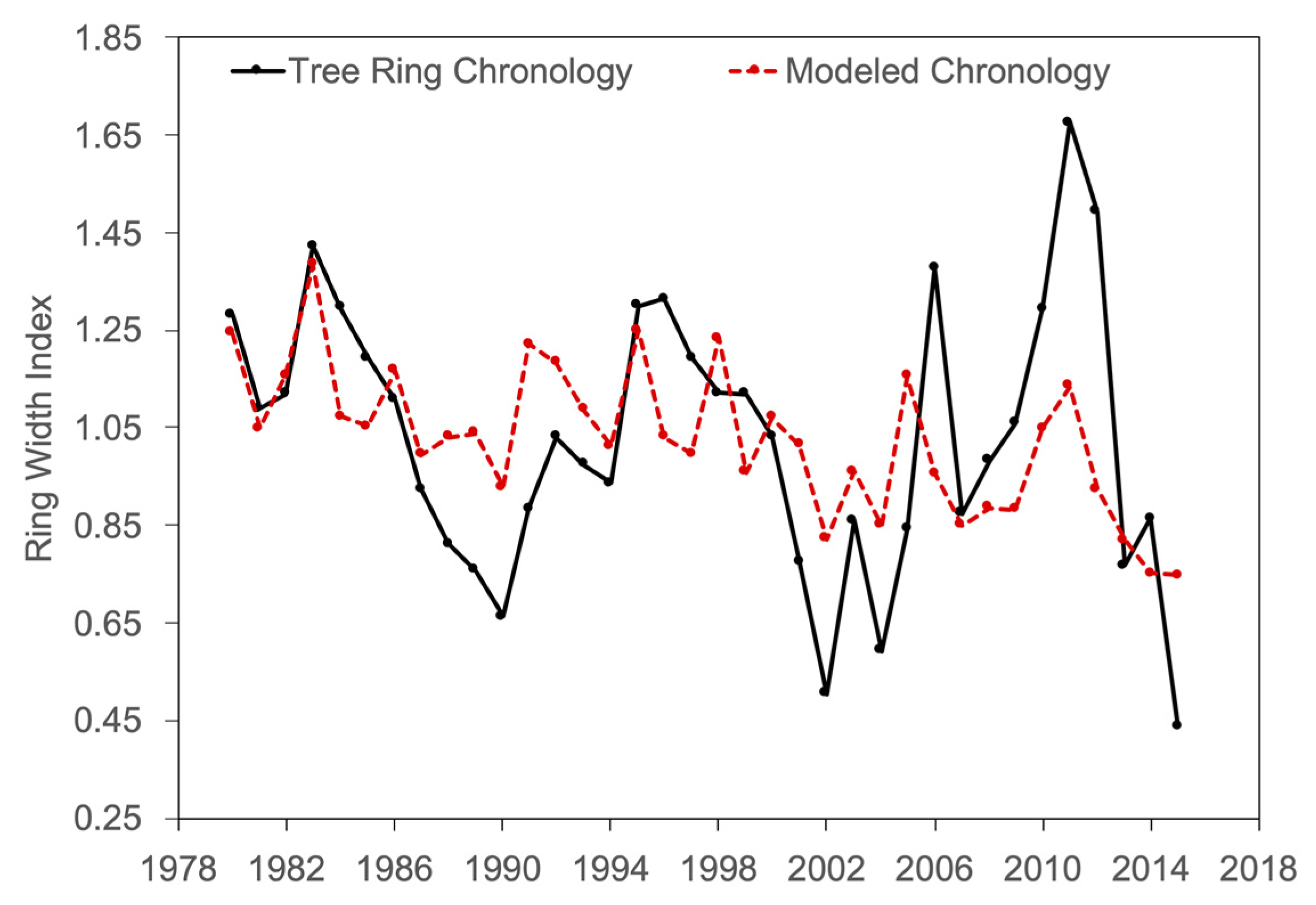
The Crestline Chronology plotted against a model of tree growth using only March PDSI and pOct–Sep NO2 based on the stepwise regression model. The correlation (r2) is 0.671, the adjusted r2 is 0.651, F = 33.66, and the standard error is 0.162.
Figure 6.
The Crestline Chronology plotted against a model of tree growth using only March PDSI and pOct–Sep NO2 based on the stepwise regression model. The correlation (r2) is 0.671, the adjusted r2 is 0.651, F = 33.66, and the standard error is 0.162.


Table 1.
Selected statistics for the Crestline ponderosa pine chronology in the San Bernardino Mountains of Southern California.
Table 1.
Selected statistics for the Crestline ponderosa pine chronology in the San Bernardino Mountains of Southern California.
| Chronology | |
|---|---|
| # Trees (# cores) | 20 (34) |
| Series length (# years) | 1855–2015 (160) |
| Mean series Series intercorrelation Sensitivity Signal to noise ratio EPS (expressed population signal) | 88.32 0.7863 0.286 13.239 0.929 |
Table 2.
Correlation coefficients between the tree ring chronology and monthly, seasonal, and annual climate trends and selected climate indices at Crestline, CA. Values in bold represent statistically significant correlations at the 95% confidence level (p < 0.05) or higher.
Table 2.
Correlation coefficients between the tree ring chronology and monthly, seasonal, and annual climate trends and selected climate indices at Crestline, CA. Values in bold represent statistically significant correlations at the 95% confidence level (p < 0.05) or higher.
| Precipitation | Temperature | SPEI | PDSI | |
|---|---|---|---|---|
| pOct | 0.12 | −0.27 | 0.22 | 0.37 |
| pNov | 0.01 | −0.09 | −0.08 | 0.30 |
| pDec | 0.14 | 0.10 | 0.08 | 0.32 |
| Jan | 0.10 | 0.00 | 0.13 | 0.35 |
| Feb | 0.29 | −0.11 | 0.26 | 0.39 |
| Mar | 0.32 | −0.16 | 0.31 | 0.46 |
| Apr | 0.09 | 0.02 | 0.05 | 0.38 |
| May | 0.00 | 0.02 | −0.02 | 0.36 |
| Jun | 0.11 | −0.06 | −0.05 | 0.32 |
| Jul | −0.12 | −0.14 | 0.00 | 0.30 |
| Aug | 0.18 | 0.00 | 0.01 | 0.28 |
| Sep | 0.05 | −0.11 | 0.02 | 0.33 |
| Oct | 0.05 | −0.20 | 0.20 | 0.28 |
| Nov | −0.03 | 0.00 | −0.10 | 0.22 |
| Dec | 0.12 | 0.11 | 0.08 | 0.22 |
| pOct–Sep (Water Year) | 0.39 | −0.15 | 0.23 | 0.42 |
| pNov–Apr | 0.37 | −0.08 | 0.29 | 0.44 |
| pOct–Apr | 0.38 | −0.14 | 0.33 | 0.44 |
| pDec–Mar (Wet Season) | 0.36 | −0.08 | 0.35 | 0.43 |
| May–Sep (Dry Season) | 0.08 | −0.09 | −0.01 | 0.35 |
| Jun–Aug | 0.16 | −0.10 | −0.02 | 0.30 |
Table 3.
Output from the stepwise regression model identifying significant variables. .
| Variable | Estimate | Std. Error | t Value | p |
|---|---|---|---|---|
| Intercept | 1.29 | 0.24 | 5.29 | p < 0.001 |
| pOct–Sep NO2 | −0.03 | 0.13 | −0.23 | p < 0.001 |
| March PDSI | 0.01 | 0.00 | 5.33 | 0.005 |
| pOct Temperature | −0.03 | 0.02 | −2.11 | 0.02 |
| pOct–Apr SPEI | 0.04 | 0.02 | 2.86 | 0.57 |
| pOct–Sep Precipitation | 0.00 | 0.00 | −0.43 | 0.67 |
| Adjusted r2 | 0.67 |
Publisher’s Note: MDPI stays neutral with regard to jurisdictional claims in published maps and institutional affiliations. |
© 2021 by the author. Licensee MDPI, Basel, Switzerland. This article is an open access article distributed under the terms and conditions of the Creative Commons Attribution (CC BY) license (https://creativecommons.org/licenses/by/4.0/).
Share and Cite
MDPI and ACS Style
Jenkins, H.S. Air Pollution and Climate Drive Annual Growth in Ponderosa Pine Trees in Southern California. Climate 2021, 9, 82. https://doi.org/10.3390/cli9050082
AMA Style
Jenkins HS. Air Pollution and Climate Drive Annual Growth in Ponderosa Pine Trees in Southern California. Climate. 2021; 9(5):82. https://doi.org/10.3390/cli9050082
Chicago/Turabian StyleJenkins, Hillary S. 2021. "Air Pollution and Climate Drive Annual Growth in Ponderosa Pine Trees in Southern California" Climate 9, no. 5: 82. https://doi.org/10.3390/cli9050082
Note that from the first issue of 2016, this journal uses article numbers instead of page numbers. See further details here.