Constraints to Vegetation Growth Reduced by Region-Specific Changes in Seasonal Climate

Abstract

We qualitatively and quantitatively assessed the factors related to vegetation growth using Earth system models and corroborated the results with historical climate observations. The Earth system models showed a systematic greening by the late 21st century, including increases of up to 100% in Gross Primary Production (GPP) and 60% in Leaf Area Index (LAI). A subset of models revealed that the radiative effects of CO₂ largely control changes in climate, but that the CO₂ fertilization effect dominates the greening. The ensemble of Earth system model experiments revealed that the feedback of surface temperature contributed to 17% of GPP increase in temperature-limited regions, and radiation increase accounted for a 7% increase of GPP in radiation-limited areas. These effects are corroborated by historical observations. For example, observations confirm that cloud cover has decreased over most land areas in the last three decades, consistent with a CO₂-induced reduction in transpiration. Our results suggest that vegetation may thrive in the starkly different climate expected over the coming decades, but only if plants harvest the sort of hypothesized physiological benefits of higher CO₂ depicted by current Earth system models.

1. Introduction

Climate change caused by increasing atmospheric carbon dioxide (CO₂) concentrations has been extensively studied in the context of global warming, and the land carbon cycle feedback is recognized as one of the biggest sources of uncertainty in climate projection [1]. Global warming is proceeding with a greening trend of the Earth, as shown by satellite and ground observations of increases in leaf area index [2,3], canopy cover [4], and biomass [5]. A greening Earth has significant consequences for the terrestrial carbon sink, the integrity of ecosystem, and climate [6,7]. Numerous mechanisms appear to underlie the observed greening, including changes in the climate system [8,9]. Among the mechanisms supporting the greening Earth, CO₂ fertilization is considered the dominant factor in enhancing vegetation, with evidence from free-air CO₂ enrich (FACE) experiments [10], satellite observations [2,4], and ground observations [11]. Climate change is also substantially contributing to the increase in global vegetation productivity because of the indirect effect of increasing CO₂ concentrations [9]. For instance, global warming is enhancing vegetation growth in high latitudes [12,13]. As such, each mechanism contributing to vegetation growth has been scrutinized independently, but, in contrast to climate change studies, the global factors affecting vegetation response have not been well studied and summarized. Therefore, the combination and interactions of multiple different climatological and biophysical mechanisms make it difficult to predict the future growth of vegetation at the global scale. As a result, the big discrepancy between modeled and observed sensitivity to CO₂ concentrations is always a source of controversy in the prediction of the future carbon cycle [14]. If climate constrains increase, climate change can cancel the positive effects of CO₂ or of other biogeochemical fertilization (e.g. nitrogen deposition) on vegetation, and possibly accelerate global warming. Therefore, understanding the relative strength of climate variables or increasing CO₂ concentrations, leading to greening or browning of the Earth, is imperative for future projections.

We firstly summarized and analyzed the trends in climate and vegetation responding to increasing CO₂ concentrations from the subset of the Coupled Model Intercomparison Project Phase 5 (CMIP5). The CMIP5 dataset includes present run and future projection data produced by Earth system models following several experimental scenarios. Future vegetation growth depends on the type, magnitude, and seasonal timing of climatic changes and their interactions with vegetation physiology. To simplify the understanding of these complex mechanisms, we divided the vegetated areas into three categories, namely temperature-limited, water-limited, and radiation-limited areas, following Nemani et al. [9].

Then, we decomposed the mechanisms enhancing vegetation growth into three factors: CO₂ concentration fertilization effect, radiative climate change, and local climate feedback by vegetation growth. By assessing these three factors quantitatively, we can answer the question as to whether increasing CO₂ concentrations will tighten or relax climate constrains on vegetation at the global scale. Friedlingstein et al. [1] evaluated the strengths of the effects of CO₂ fertilization and temperature increase on land vegetation carbon storage. Lemordant et al. [15] decomposed the climate effects on evapotranspiration into net radiation, precipitation, and vapor pressure deficit (VPD). However, none of them counted the local climate feedback effect at the global scale. Therefore, contradicting results of vegetation growth by different mechanisms made future predictions confusing. For instance, it is hard to discuss the regional trend in precipitation [16,17,18] and the changes in water use efficiency [11] at the same time without knowing which mechanism is relatively stronger. Finally, we discussed the validity of the findings through the analysis of historical observations.

2. Materials and Methods

2.1. CMIP5

CMIP5 is a set of model experiments for assessing past and future climate change in the Intergovernmental Panel for Climate Change Assessment Report number 5 (IPCC AR5) [19]. To objectively select datasets, the models of CMIP5 data used in this paper met the following criteria.

• The models had monthly data of near-surface air temperature (output variable name in the standard output is tas; the other variables are showed the same way hereafter), precipitation (pr), surface downwelling shortwave radiation (rsds), and Leaf Area Index (LAI) (lai) data for the specific years (1875–2005: historical; and 2006–2099: Representative Concentration Pathway (RCP) 8.5).
• The land sub-model had year-to-year changes in LAI.

We used three sets of outputs from 21 models from CMIP5 (

Table 1. Coupled Model Intercomparison Project Phase 5 (CMIP5) models and the forcing characteristics. Models used in the sensitivity analysis (experiment IDs are esmFixClim1, esmFdbk1, and 1pctCO2) shown in the analysis are highlighted in red.

Model	Modeling Group	Land Component	N Cycle	Dynamic Vegetation
bcc-csm1-1	Beijing Climate Center, China Meteorological Administration, CHINA	AVIM1.0	N	N
bcc-csm1-1-m	Meteorological Administration, CHINA	AVIM1.0	N	N
BNU-ESM	Beijing Normal University, CHINA	CoLM3 & BNU DGVM (C/N)	-	-
CanESM2	Canadian Center for Climate Modelling and Analysis, CANADA	CLASS2.7 & CTEM1	N	N
CESM1-CAM5	Community Earth System Model Contributors, NSF-DOE-NCAR, USA	CLM4	Y	N
CESM1-WACCM	Community Earth System Model Contributors, NSF-DOE-NCAR, USA	CLM4	Y	N
CESM1-BGC	Community Earth System Model Contributors, NSF-DOE-NCAR, USA	CLM4	Y	N
GFDL-CM3	NOAA Geophysical Fluid Dynamics Laboratory, USA	LM3	N	Y
GFDL-ESM2G	NOAA Geophysical Fluid Dynamics Laboratory, USA	LM3	N	Y
GFDL-ESM2M	NOAA Geophysical Fluid Dynamics Laboratory, USA	LM3	N	Y
HadGEM2-ES	Met Office Hadley Centre, UNITED KINDOM	MOSES2 & TRIFFID	N	Y
INMCM4	Russia
IPSL-CM5A-LR	Institut Pierre-Simon Laplace, FRANCE	ORCHIDEE	N	N
IPSL-CM5A-MR	Institut Pierre-Simon Laplace, FRANCE	ORCHIDEE	N	N
MIROC5	JAMSTEC, University of Tokyo, and NIES, JAPAN	MATSIRO & SEIB-DGVM	N	Y
MIROC-ESM-CHEM	JAMSTEC, University of Tokyo, and NIES, JAPAN	MATSIRO & SEIB-DGVM	N	Y
MIROC-ESM	JAMSTEC, University of Tokyo, and NIES, JAPAN	MATSIRO & SEIB-DGVM	N	Y
MPI-ESM-LR	Max Planck Institute for Meteorology, GERMANY	JSBACH	N	Y
MPI-ESM-MR	Max Planck Institute for Meteorology, GERMANY	JSBACH	N	Y
MPI-ESM1	Max Planck Institute for Meteorology, GERMANY	JSBACH	N	Y
NorESM1-ME	Norwegian Climate Centre, NORWAY	CLM4	Y	N
NorESM1-M	Norwegian Climate Centre, NORWAY	CLM4	Y	N

).

The experiments are:

1. Historical run: Runs covering the historical period 1850–2005. For this period, model forcings include: greenhouse gases (GHG), volcanoes, aerosols, and land cover.

2. RCP 8.5: Projections forced by pre-determined increasing CO₂ concentrations covering 2006 to 2100. For this analysis we chose the RCP 8.5 scenario, a pathway with the highest greenhouse gas emissions, leading to 8.5 W/m² radiative forcing at the end of the 21^st century [20]. Although just a decade passed since 2006, it has been reported that the emission concentration in 2100 is projected to follow RCP 8.5 [21].

3. Sensitivity experiments: In order to assess the contribution of CO₂ fertilization and climate effects on vegetation separately, we used an eight-model (highlighted in Table 1) ensemble to compare three CMIP5 experiments, each of which was run for 140 years and experiences a constant CO₂ of preindustrial level and/or CO₂ increasing by 1%/year to 4xCO₂: (1) In the fertilization experiment CO₂ increases by 1%/year to 4xCO₂ for the land surface, but stays constant at preindustrial level for the atmosphere, and thus the climate effect is suppressed and the CO₂ fertilization effect is dominant on land (the official experiment ID is esmFixClim1); (2) in the climate experiment CO₂ increases for the atmosphere, but stays constant for the land surface, and hence the CO₂ fertilization effect is suppressed and the climate impact dominates (esmFdbk1); (3) in the combined experiment CO₂ concentration increases for the full Earth system (1pctCO2).

To calculate the ensemble mean, at first, we remapped all the CMIP5 data into quarter degree grid data using the bilinear interpolation method. Then, we calculated the ensemble mean for each quarter degree grid from the available modeled data.

In this paper, gross primary production (GPP) was chosen from available CMIP5 land variables as the representation of photosynthesis. GPP is the amount of photosynthesis by vegetation per unit area, from which respiration is not subtracted. In the budget analysis, net biome production (NBP), which accounts for respiration and disturbance, should be the key flux of vegetation response. However, these experiments are not CO₂ emission driven, but rather CO₂ concentration driven, and the results of the carbon budget of vegetation do not change the atmospheric CO₂ concentration. Thus, GPP, which is equivalent to photosynthesis, can represent vegetation growth better than NBP. We also used LAI as the representative of carbon storage because LAI can be compared to satellite estimates.

The vegetation response in the historical run, RCP 8.5, and combined experiments in sensitivity experiments can be simplified by the linear models as follows:

$$\Delta GPP = a \Delta C{O}_2 + b \Delta Clim + f \Delta Cli{m}_{feedback},$$

(1)

where $\Delta C{O}_2$, $\Delta Clim$, and $\Delta Cli{m}_{feedback}$ represent change in CO₂ concentration, change in one of the limiting climate factors but only caused by the radiative effect of the change in CO₂ concentration, and feedback of climate by changing GPP through the fertilization effect, respectively. The coefficients a, b, and f assume a simple linear system. The term $\Delta Cli{m}_{feedback}$ represents the feedback of GPP through effects on climate, such as the effect of a change in cloud cover due to increasing evapotranspiration.

The fertilization experiment examines how higher CO₂ affects climate and vegetation via increases in leaves’ internal CO₂ concentration, which should in turn reduce stomatal conductance transpiration. As a result, climate feedback occurs as decreasing cloud cover whilst increasing soil moisture, runoff, and solar radiation [11,22,23]. So, the fertilization experiment can be expressed as:

$$\Delta GPP = a \Delta C{O}_2 + f \Delta Cli{m}_{feedback},$$

(2)

It is noteworthy that $\Delta C{O}_2$ includes the effect of changing water use efficiency because it is directly affected by increasing CO₂ concentrations, not through changing climate.

The climate experiment shows how higher CO₂ affects vegetation via the traditional greenhouse effect on climate. The fertilization effect of increasing CO₂ on vegetation was suppressed. The climate experiment can be expressed as:

$$\Delta GPP = b \Delta Clim,$$

(3)

For mapping purposes, the outputs were firstly re-gridded to 0.5 × 0.5 degree resolution, using the bilinear interpolation method, to be consistent with the limiting factor data [9].

2.2. GIMMS-LAI3G

The GIMMS-LAI3G data were derived from the Global Inventory Modeling and Mapping Studies (GIMMS) Normalized Differential Vegetation Index (NDVI) using the neural network algorithm [24]. We aggregated the 1/12 degree spatial resolution LAI data into the half degree data prior to monthly and annual analysis. To be consistent with historical CMIP5 runs that end in 2005, we used GIMMS-LAI3g data from overlapping the period 1982–2005.

2.3. CRU/CRUNCEP

We used 0.5 × 0.5 degree monthly temperature and precipitation from Climate Research Unit (CRU-TS3.23) and solar radiation data from CRU National Centers for Environmental Prediction version 4 (CRUNCEP-V4, a blend of CRU data and NCEP- National Center for Atmospheric Research (NCAR) reanalysis data) [25]. CRU data are interpolated gridded datasets from monthly observations. To be consistent with historical CMIP5 runs, we used CRU/CRUNCEP data from overlapping the period with Global Inventory Modeling and Mapping Studies (GIMMS)-LAI data during 1982–2005.

2.4. NDP026

We reanalyzed the ground-based total cloud cover observations in Numeric Data Package NDP06 [26], following methodology outlined in Warren et al. [27]. Briefly, the methodology consists of estimating seasonal trends at each of the stations, then averaging these trends over a 10 × 10 degree grid. We compared these estimated trends with those predicted by CMIP5 models for the period of 1971–2005 using a chi-squared test for independence. Several modeling studies showed the connection between low clouds over land and increased levels of CO₂ in the atmosphere [28,29]. As such, it would have been more appropriate to use changes in low cloud cover in our analysis. However, CMIP5 did not mandate modeling teams to submit low, medium, and high cloud simulations separately. Only total cloud cover was required from the modeling teams, hence we used total cloud cover data in our analysis.

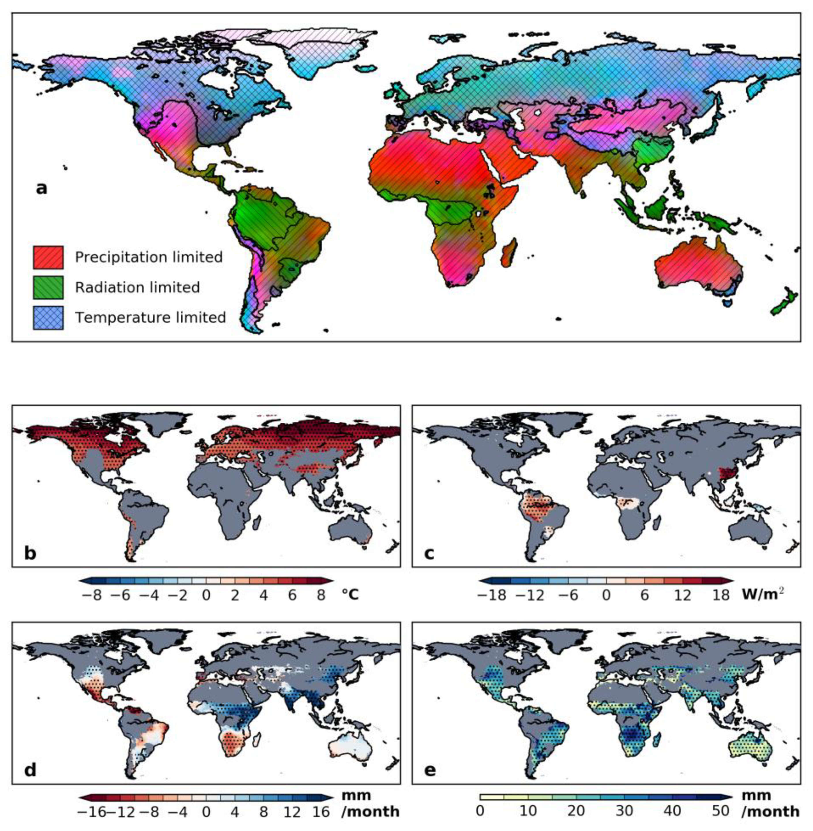
2.5. Limiting Factor Analysis

We analyzed global changes in the three regions defined by the climate factor—temperature, precipitation, or radiation—that is most limiting to GPP. Following Nemani et al. [9], we calculated the strength of the limiting factor based on monthly climate data of minimum temperature, precipitation, and cloudy day. Then, we defined the three regions using the highest value among the three data (Figure 1a).

2.6. Estimation of Precipitation Equivalent Water

Increases in atmospheric CO₂ are known to increase the water use efficiency (WUE) of vegetation, estimated as amount of carbon gained per unit amount of water used [11,22,30]. While WUE increases globally with CO₂, its changes over precipitation-limited regions are of particular significance for plant growth. To assess the contribution of improved WUE in precipitation-limited regions, we used a slightly different metric called precipitation use efficiency (PUE). PUE is estimated as GPP per unit amount of precipitation. The changes in PUE between the first (2006–2015) and last decades (2090–2099) are then translated to changes in precipitation equivalent, $P{E}_q$ (mm), as follows:

$$P{E}_q=\left(GP{P}_{last}-GP{P}_{first}\right)\times \frac{P_{first}}{GP{P}_{first}}-\left( P_{last}-P_{first}\right),$$

(4)

where $GP{P}_{first}$ and $GP{P}_{last}$ are GPP (kgC/m²) for the first and last decades of the 21st century, and $P_{first}$ and $P_{last}$ are precipitation received at each of the grid cells during the first and last decades.

2.7. Mann–Kendall Test

The Mann–Kendall test detects the presence of a monotonic trend in time-series data [31]. The test is broadly used because it does not require the assumption of normal distribution of the time-series data. We use the Mann–Kendall test as the significance test for the annual or seasonal data.

3. Results

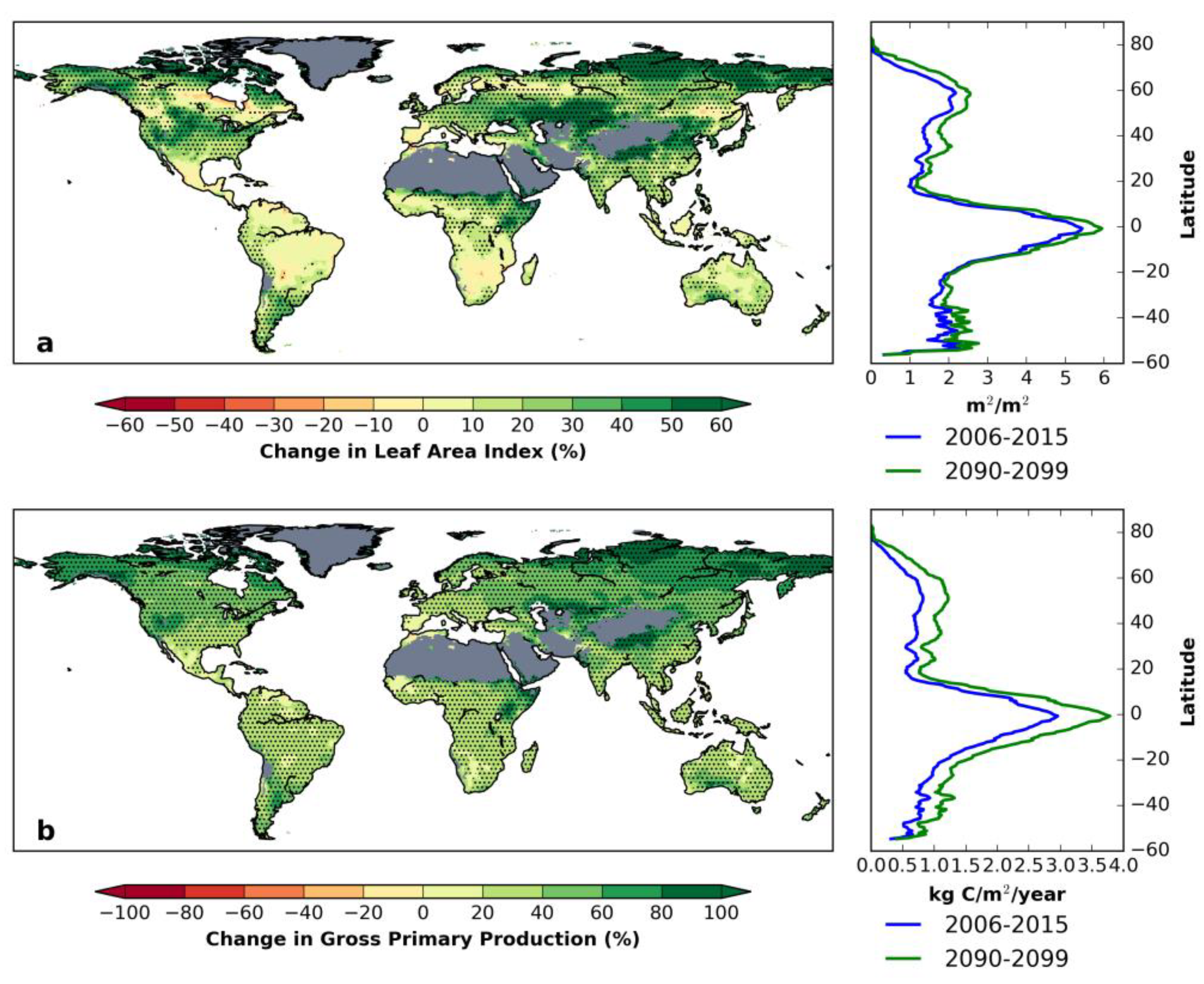
3.1. Annual Mean Trend and Climate Feedback to Vegetation

The multi-model ensemble mean shows pervasive future changes in vegetation structure and function by the end of this century under the high-emission RCP 8.5 scenario: LAI increases by up to 60% and GPP increases by up to 100% (Figure 2). LAI significantly increases globally except for Amazon, Mexico, and Southern Africa (Figure 2a). GPP also significantly increases for nearly the entire vegetated planet (Figure 2b), though the magnitudes may be uncertain [32]. The percentage changes are higher in the high latitude regions for LAI, while changes in magnitude of LAI and GPP are higher in both the high latitude and tropical regions. A few tropical and semi-arid areas show decreases in LAI, but none of the changes are statistically significant. The results of increasing LAI are consistent with Mahowald et al. [33].

We divided the climate (Figure 3) and the vegetation (Figure 4) response in the RCP 8.5 scenario into the temperature-limited, precipitation-limited, and radiation-limited regions. Temperature and precipitation increase for all the three regions, while radiation increases only in the radiation-limited area (Figure 3). Thus, all the climate factors contribute to vegetation growth in addition to the CO₂ fertilization effect. As a result, all the three different climate-limited regions experience increases in ensemble GPP and LAI throughout the 21st century (Figure 4). LAI in the temperature-limited region shows large variability among the models compared to GPP, which implies the difficulty in modeling respiration and allocation ratios. LAI in the radiation-limited region shows a significant increase, but the magnitude of increase is small due to the saturation of the leaf increase.

By the last decade of the 21st century, the summary of the projections shows that annual climate constraints will ease for 51% of the Earth’s vegetated land area (i.e., warmer in the temperature-limited region), tighten in 11% of the land area, with the remainder experiencing no change. The degree of easing varies, from 94% in the temperature-limited region and 23% in the precipitation-limited region, to 45% in the radiation-limited region (Figure 1b–d).

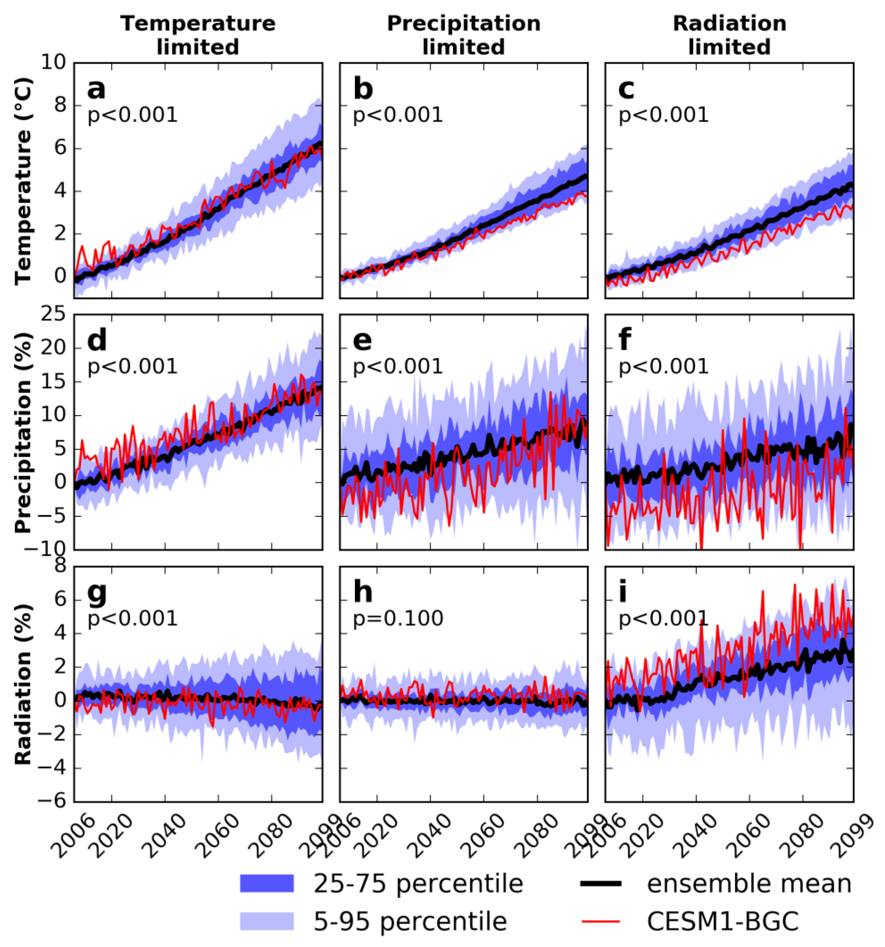
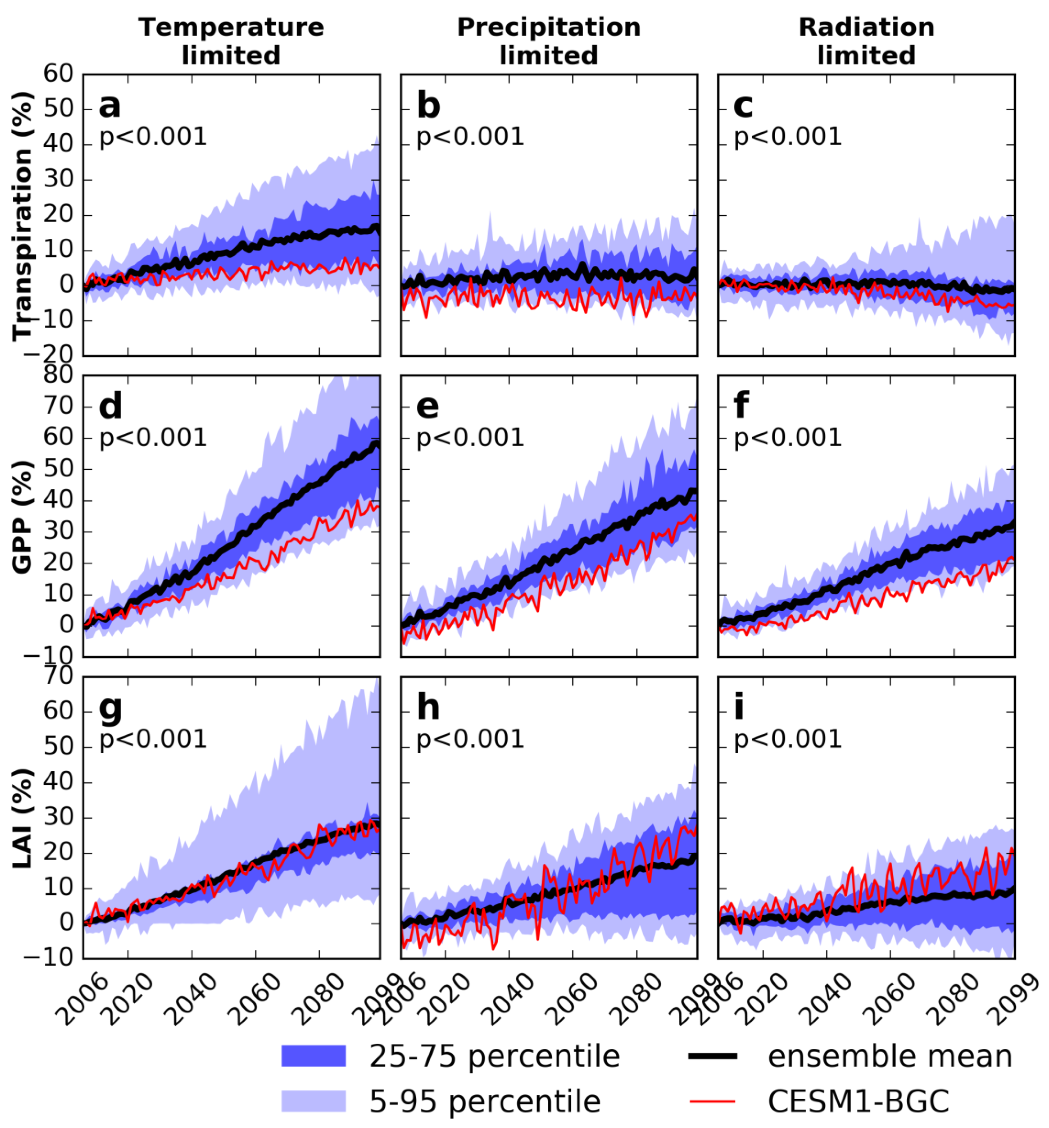
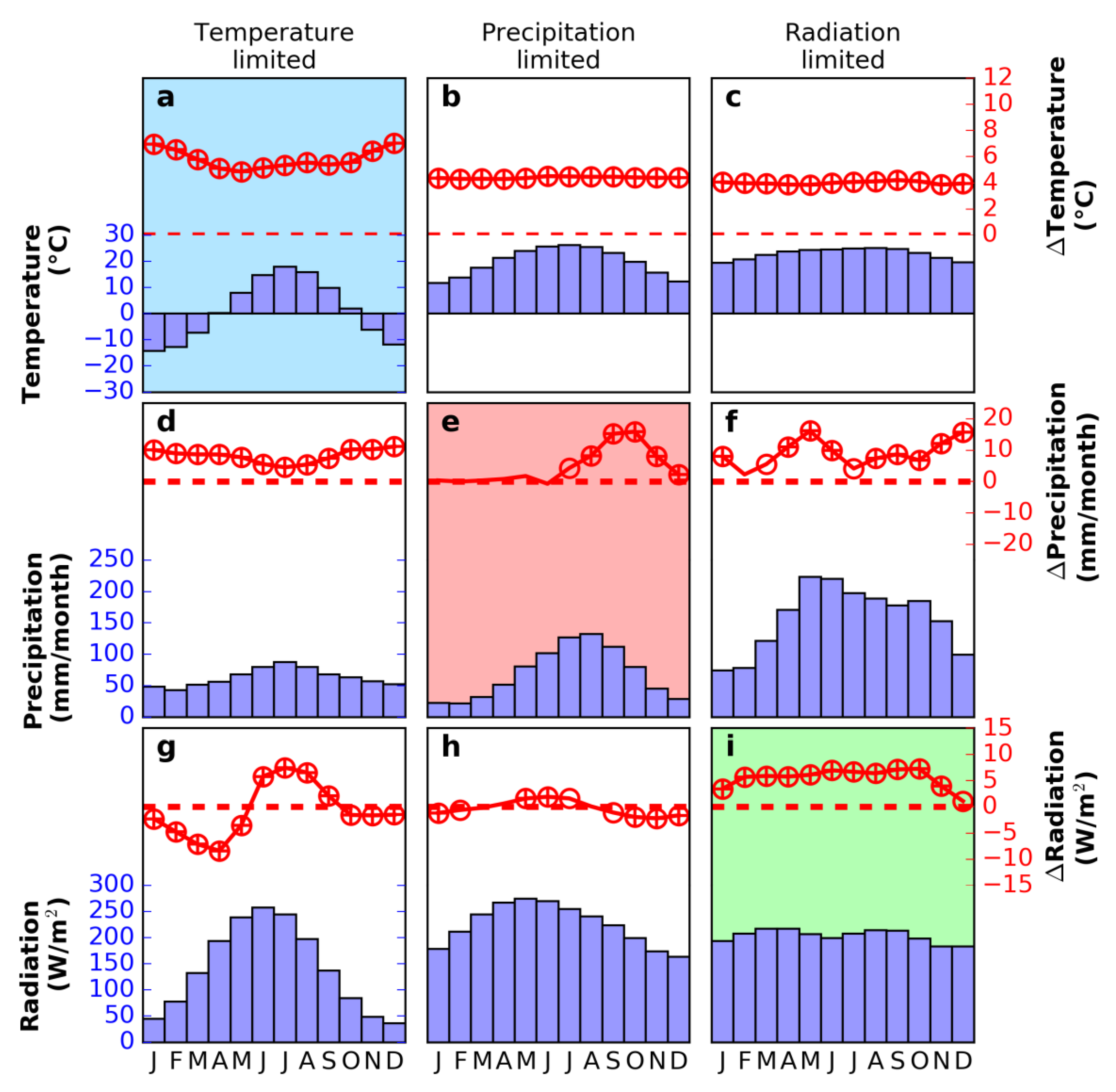
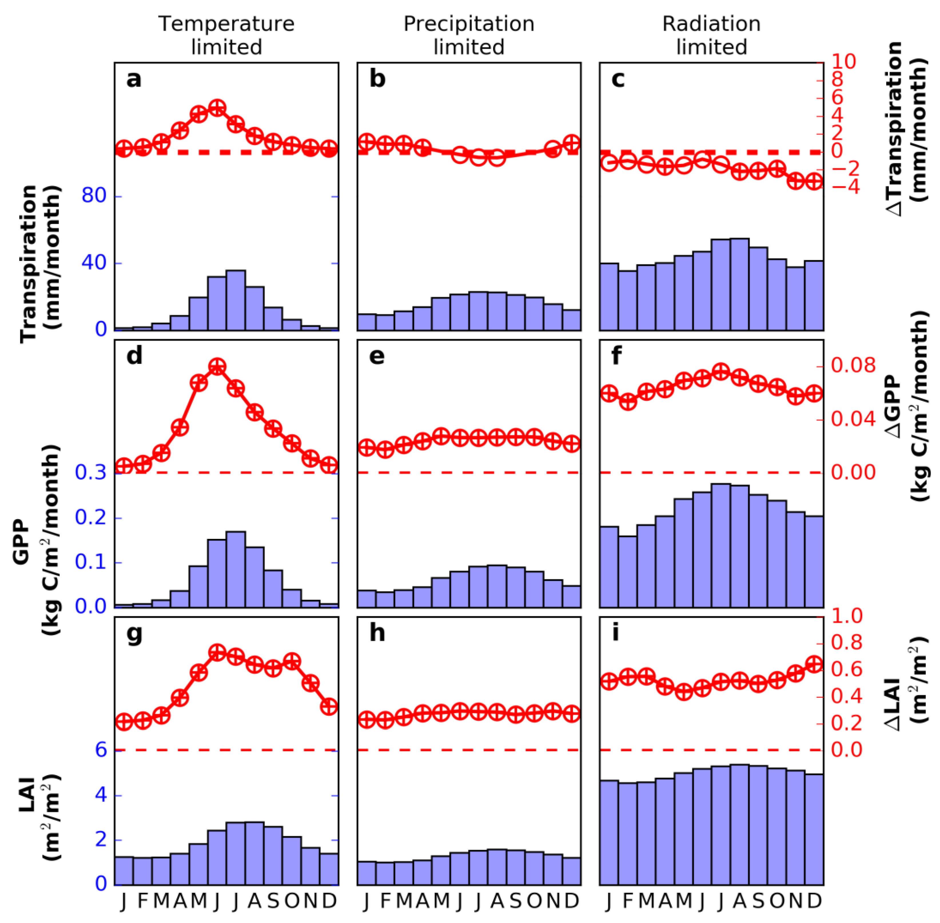
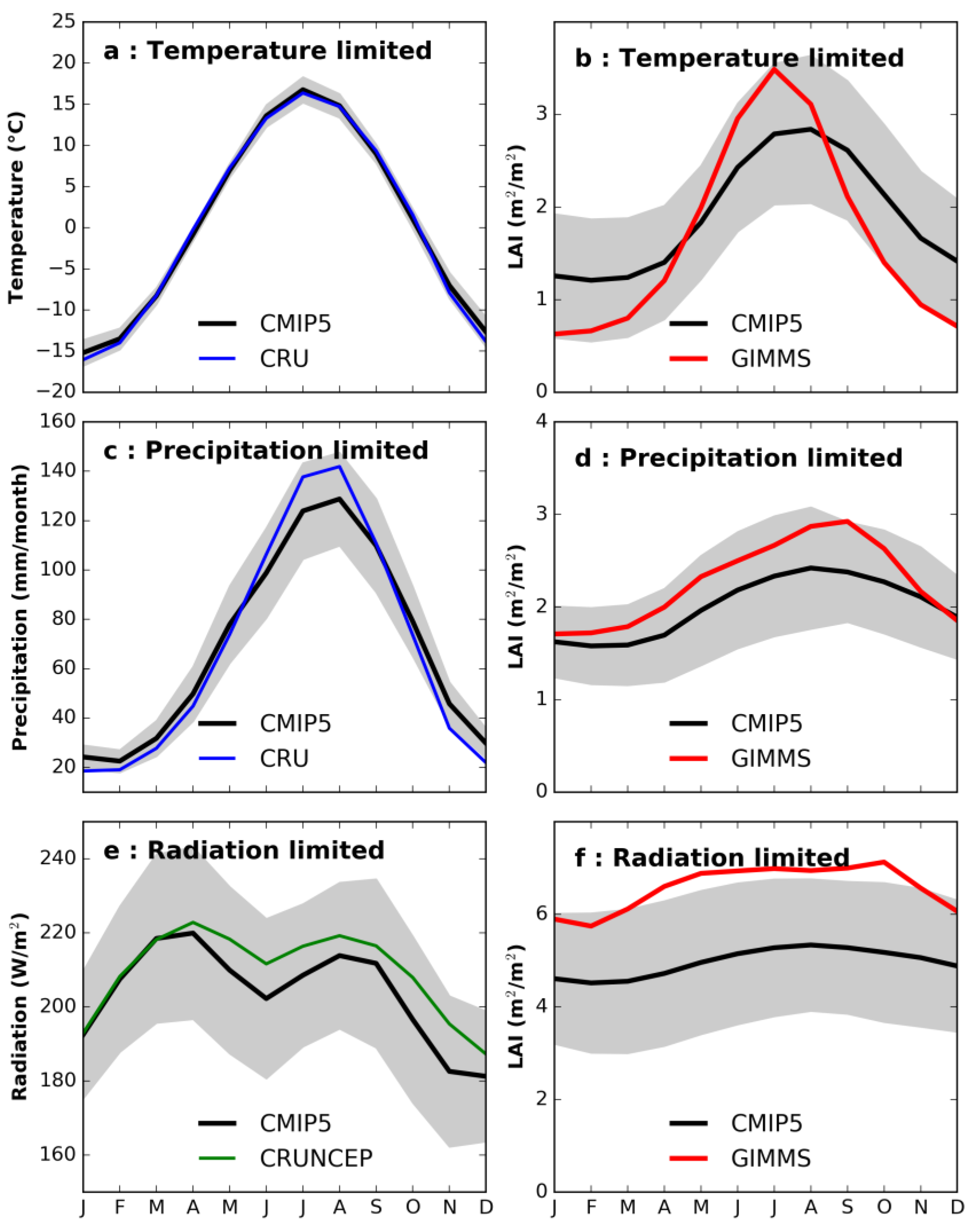
3.2. Seasonal Trend in Climate and Vegetation

The changes in LAI and GPP are underlain not only by changes in annual climate but also by seasonal climate changes. Seasonal changes in climate (Figure 5) are associated with increased LAI and GPP (Figure 6), particularly for the temperature-limited region (note that we present seasonal analyses for the Northern Hemisphere only, to avoid contrasting seasonal patterns in the Southern Hemisphere and because the Northern Hemisphere accounts for 68% of total land area).

Boreal summers (June, July, and August: JJA) in temperature-limited regions become warmer, wetter, and brighter (Figure 5a,d,g); conditions that, at least in current Earth system models, lead to a summertime spike in LAI and GPP increases (Figure 6m,p). The precipitation increase is largest in the boreal fall (September, October, and November: SON); warming is at least 4 °C in all months, and increases to nearly 10 °C in winter. The JJA increase in solar radiation approaches 10 W/m², but is offset by winter decreases (Figure 5g), leading to no net change in the annual mean (Figure 3g).

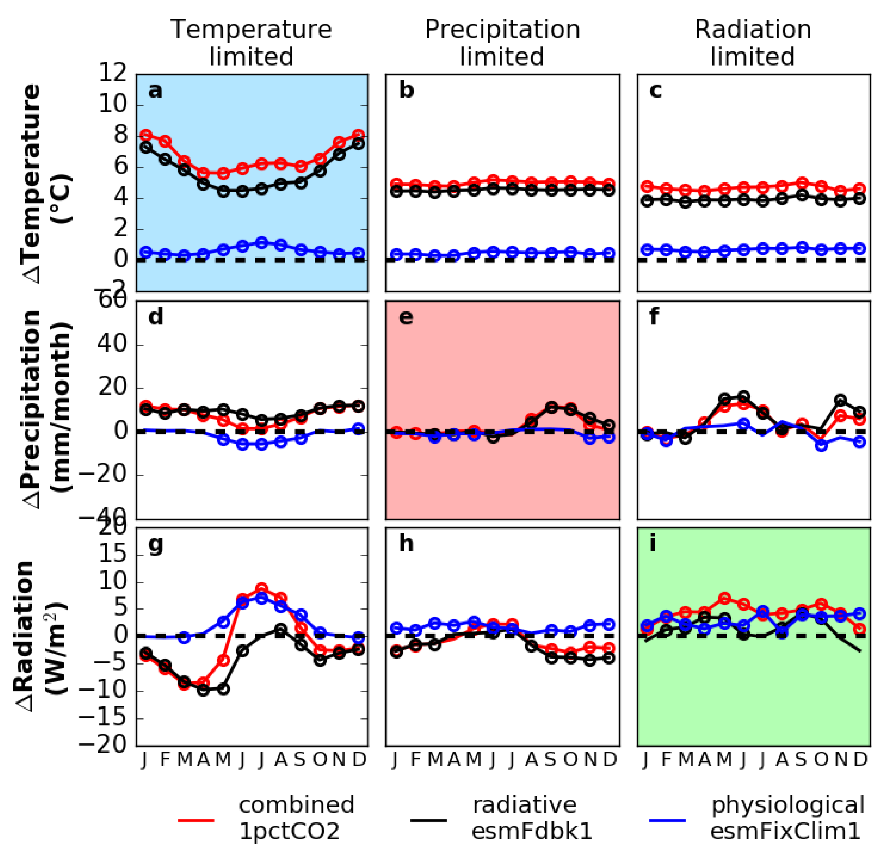
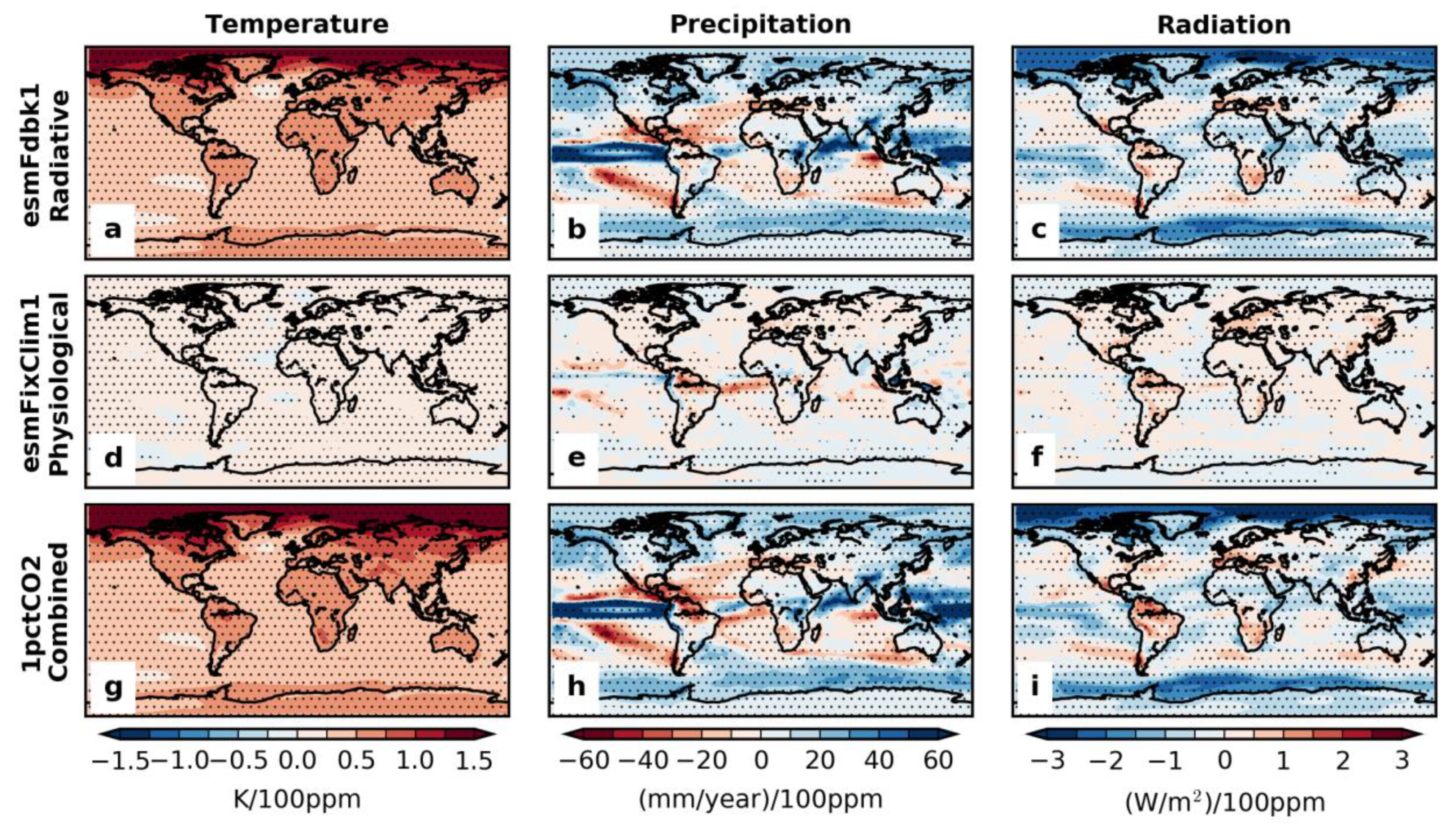
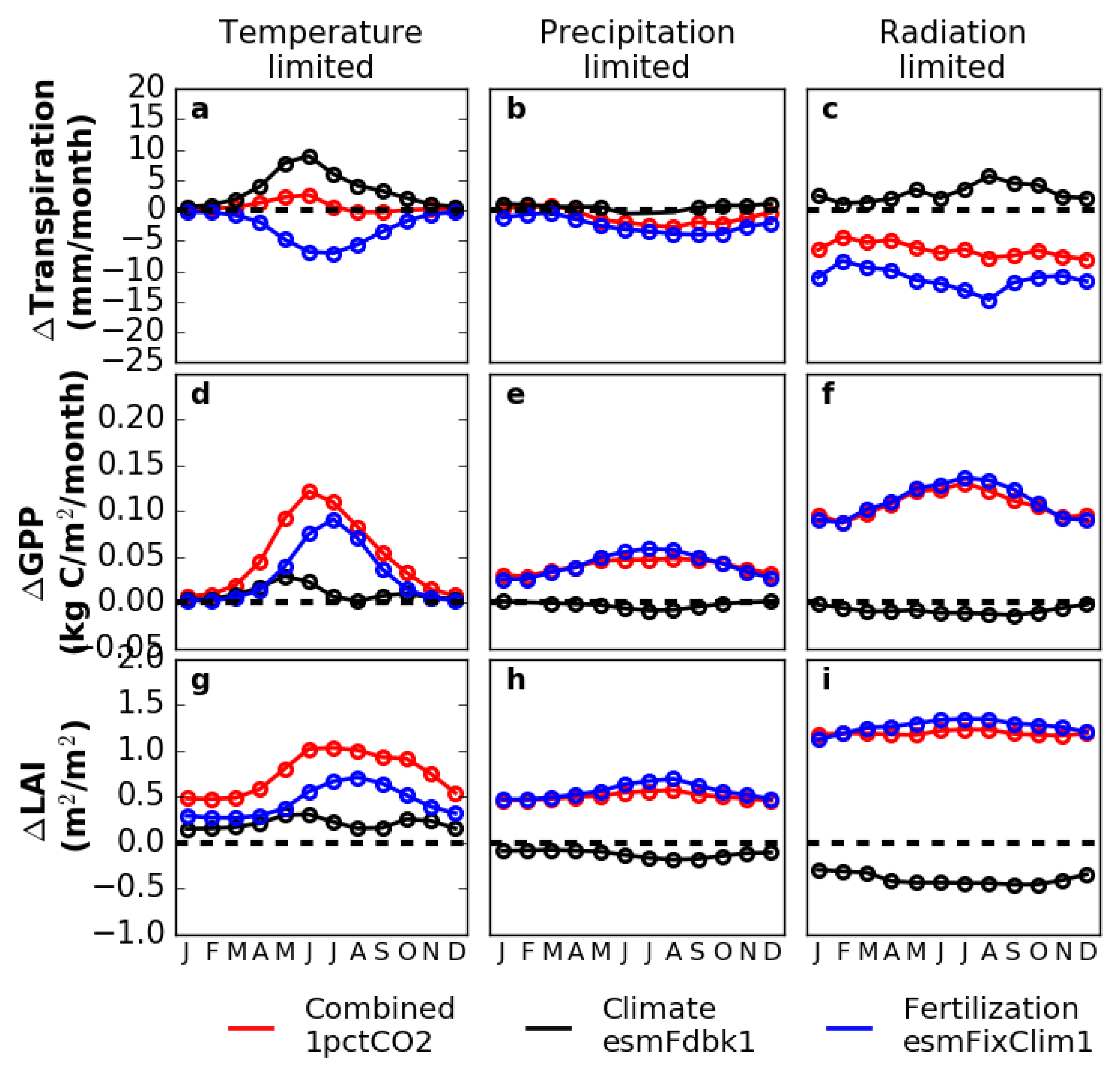
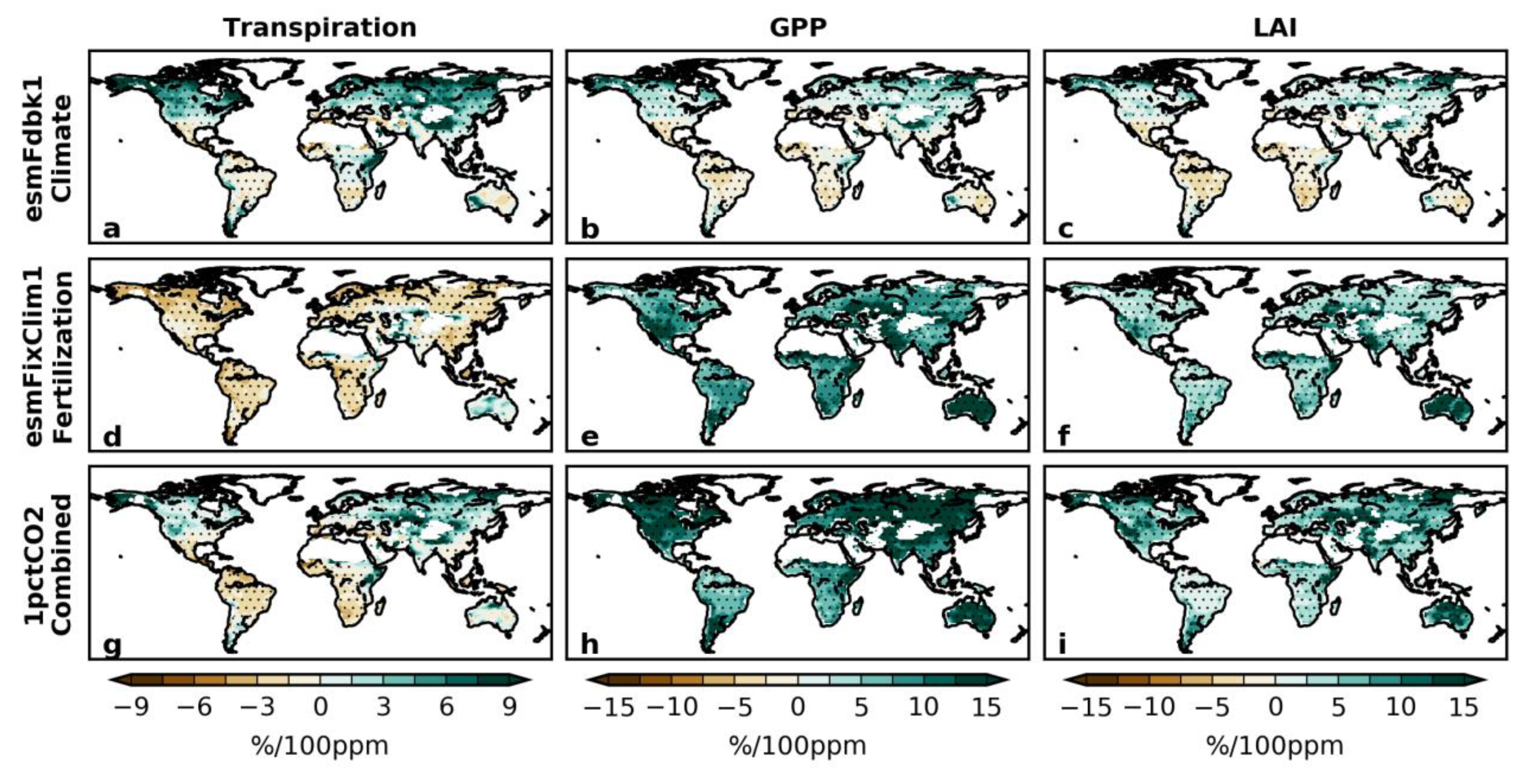
3.3. Sensitivity Experiments for Climate and Vegetation

Increased CO₂ affects LAI and GPP through climate change, through both the greenhouse effect and CO₂ fertilization effect, but the CMIP5 ensemble for the RCP 8.5 scenario cannot separate the importance of the two processes [19]. To isolate their varying importance, we generate an eight-model ensemble (highlighted in Table 1), comparing results from the sensitivity experiments.

At first, we summarized the climate responses to increasing CO₂ concentration in these sensitivity experiments. The esmFdbk1 experiment shows that radiative effects clearly dominate projected warming, the signature feature of climate change (compare black and red lines in Figure 7a–c and Figure 8a,d,g). Radiative effects also drive other key aspects of climate change, such as Arctic amplification and land–sea warming contrast (Figure 8a), equatorial and high-latitude increases in precipitation (Figure 8b), and high-latitude dimming from increases in fall/winter cloud cover (Figure 8c) [34]. Meanwhile, the esmFixClim experiment revealed that, except for increases in radiation for the temperature-limited region in JJA (Figure 7g), the vegetation physiological effect has little effect on region-averaged climate (e.g., near-zero changes in Figure 7a–f). Spatially, the physiological effects on climate are more consistent than the radiative effects, and include a slight drying (Figure 8e) and brightening because of reduced cloud cover (Figure 8f) over most land surfaces.

On the other hand, the summary of the vegetation response to increasing CO₂ concentration shows the opposite of the climate response in the sensitivity experiment. In spite of inducing climate changes to temperature and precipitation, the CO₂ fertilization effect alone can account for much, and in some cases, almost all, of the simulated changes in GPP and LAI in the combined experiment (compare blue and red lines in Figure 9d–i). Increases in LAI and GPP in the FixClim1 experiment appear to be driven by more radiation (because of reduced cloud cover) and reduced transpiration (therefore increased soil water), both of which are consistent with stomatal down-regulation following CO₂ increases [35]. As shown in the esmFdbk1 experiment, in contrast, the climate change induced by radiative forcing has near-zero effects on simulated GPP for all three regions (black line in Figure 9d–f), except for a small positive effect on GPP in the boreal spring of the temperature-limited region. Spatially, the ordinal impact on GPP and LAI often reverses between the esmFdbk1 and esmFixClim1 experiments, with much of the Southern Hemisphere switching from a reduction (Figure 10b,c) to an enhancement (Figure 10e,f).

For seven out of nine comparisons, the esmFdbk1 and esmFixClim1 experiments produce offsetting impacts on LAI and GPP (Figure 9). The largest differences are in the radiation-limited region, where the esmFdbk1 experiment slightly reduces GPP and the esmFixClim1 experiment increases GPP by as much as 0.15 kg C/m²/month in JJA (compare blue and red lines in Figure 9f); LAI changes switch from about −0.5 to 1.0 (compare blue and red lines in Figure 9i). The temperature-limited region is an exception, where, for both LAI and GPP, the esmFdbk1 and esmFixClim1 experiments are additive (Figure 9m,p). In particular, high northern latitudes are the one clear location where both the esmFdbk1 and esmFixClim1 experiments increase LAI (Figure 10c,f) and GPP (Figure 10b,e), supporting recent conclusions of a strong climate imprint on the broad region of high-latitude during the observational era [36].

Figure 10. Spatial distribution of the additive and counteracting impacts of CO₂ on vegetation. Same as Figure 8 except for transpiration, a, d, g; GPP, b, e, h; and LAI, c, f, i.

Figure 10. Spatial distribution of the additive and counteracting impacts of CO₂ on vegetation. Same as Figure 8 except for transpiration, a, d, g; GPP, b, e, h; and LAI, c, f, i.

The critical role of vegetation physiology is clear in the precipitation-limited region, which experiences the least easing and an almost equal area with precipitation reductions (Figure 1d). But the region also sees a statistically significant increase in simulated equivalent precipitation water in 64% of its area (equivalent to up to 50 mm/month of water in some areas, Figure 1e) and increases in LAI and GPP (Figure 9e,h), in spite of near-zero changes in simulated annual (Figure 4b) and seasonal (Figure 6b) transpiration. While these patterns depict a more efficient use of available water resources and a progressive greening, the physiological response of plants to higher CO₂ in semi-arid regions appears to depend on local variations in simulated precipitation, which remain highly uncertain in CMIP5 simulations [37].

3.4. Decomposing Vegetation Growth Into Three Factors

The results indicate that the climate feedback substantially contributed to the growth of vegetation by relaxing climate constraints. Although it is well known that the climate feedback can positively or negatively influence the growth of vegetation, it has not been quantitatively assessed at the global scale. The sensitivity experiments allow us to quantitatively evaluate the climate feedback to vegetation ($f \Delta Cli{m}_{feedback}$ in Equation (1)). We assumed that the ratio of GPP change to change in climate variables is constant (i.e., b = f = const.). At first, we calculated $\Delta GPP / \Delta Clim$ (i.e., b) in the climate experiment using the linear regression of annual GPP on annual mean climate variables. Then, we calculated $a \Delta C{O}_2$ by subtracting $f \Delta Cli{m}_{feedback}$ from GPP increase in Equation (2). Finally, $b \Delta Clim$ was derived from Equation (3) by subtracting $a \Delta C{O}_2$ and $f \Delta Cli{m}_{feedback}$ by assuming the additive relationship of the fertilization effect and the climate change effect.

The percentage ratios of the contribution of each term (i.e., $a \Delta C{O}_2$, $b\Delta Clim$, and $f \Delta Cli{m}_{feedback}$) were shown for each limited region in Figure 11. In the temperature-limited region, all the three terms substantially contributed to the increase in GPP, and the annual average of the climate feedback contribution was 17%. The snow-albedo feedback can account for the climate feedback [38,39]. The climate feedback added 37% more increase in GPP than the radiative warming effect alone. The total contribution of climate feedback and climate is 63%, which is the highest contribution among the three climate-limited regions. The contribution is much higher in winter than summer because the temperature did not limit GPP in the summer.

In the precipitation limited area, there was almost no contribution of the climate feedback effect. This result can be explained by the relatively low water-recycling ratio compared to the humid area [40]. The moisture from the other regions controls the precipitation trend in the water-limited region, so that the influence of changing water use efficiency on the region is negligible.

In the radiation-limited area, the contribution of the climate feedback is 7%, while the radiative climate change negatively affects 24% of the increase in GPP. The feedback was caused by the decreasing trend in cloud cover through change in water use efficiency [35]. The magnitude of the contribution of the climate feedback changes with model selection due to the difficulty in modeling clouds in GCMs. Thus, the feedback contribution can be underestimated, especially when a low resolution GCM cannot represent well the increase in regional convective clouds caused by the enhanced water cycle that results from added vegetation growth.

4. Discussion

Our analysis suggests fundamental future increases in the amount of vegetation and photosynthesis (LAI and GPP in Figure 1), mainly arising from relaxing climate constraints on vegetation growth. This feedback effect can explain the discrepancy between the models and the observation in the β factor [14]. We argue that the results are consistent with three lines of observational evidence and a considerable body of paleoclimatic evidence of dramatically different vegetation composition during past high-CO₂ periods [41,42].

First, if our central claim that vegetation physiological process reduces transpiration, reduces cloud cover, and increases radiation is correct, then cloud cover, particularly low-level clouds, which strongly influence the planetary shortwave radiation budget, should decrease. Recent climate modeling studies indeed simulate a decrease in low-level cloudiness due to the vegetation physiological effect [23,29,35]. Further, several modeling studies indicate that the rapid adjustments of the troposphere for the combined radiative and physiological effects of increased CO₂ are associated with a decrease in low-level cloud cover over land, but increased boundary layer cloud cover over oceans [29,43,44]. We re-analyzed the NDP026 ground observation of cloud cover [26] and show that the modeled processes have indeed occurred over the period 1971 to 2005 using the Mann–Kendall trend test,. During this period, cloud cover significantly decreased by a few percent points per decade over much of the land surface, and increased over the ocean (Figure 12).

Second, the same models we used for future projections under RCP 8.5 produce simulations of the historical climate and vegetation that are broadly consistent with independent observations (Figure 13). Although historical skill does not guarantee future performance, region-level simulations of climatological temperature, and precipitation are statistically indistinguishable from the Climate Research Unit (CRU) product [25] in all months (Figure 13a,b). Simulated radiation, assessed for the radiation-limited regions of the Northern hemisphere against the CRUNCEP radiation dataset, has climatological differences of up to 15 W/m², but a similar seasonal cycle (Figure 13e). The Earth system models also capture seasonal satellite-observed variations in LAI in all three regions (Figure 13b,d,f).

Third, the projected changes in LAI and climate are already apparent in the observational era. Satellite data show that LAI has increased from 1982 to 2005 for all three regions (Figure 14b,d,f); the CRU product shows warming in the temperature-limited region (Figure 14a), increased precipitation in the precipitation-limited region (Figure 14c), and reduced cloud cover in the radiation-limited region (Figure 14e). Consistent with these changes in climate and the biosphere, terrestrial ecosystems have been shown as net sink for carbon in recent decades [45,46]. Thus, the 21st century changes to climate and greening do not appear anomalous or implausible, when viewed in the context of recent history.

Numerous processes, including extreme climatic events [47], could reduce the projected changes in LAI and GPP. But the paleoclimate record also shows that profound changes in vegetation have occurred in the past, particularly in high latitudes, where the temperature-limited region appears to benefit the most from physical climate changes, mediated through vegetation physiological mechanisms. The early Eocene greenhouse climate, for example, supported redwoods at 78° N paleo-latitude under CO₂ levels that are similar to the modern levels [42]. The deep-time perspective, albeit associated with different time scales and continental configurations, therefore, does not appear to rule out the sort of major changes to vegetation seen in the 21st century projections [48].

We focused on two elemental components of terrestrial ecosystems—the amount of leafy material and gross carbon fixation—but do not provide insights into respiratory and net carbon fluxes, carbon stocks, such as biomass and soil carbon, and vegetation dynamics. The CMIP5 models, especially low-resolution models, cannot count the extreme events, such as forest fires or hurricanes. The FACE experiments also suggest that non-climate limiting factors, such as nitrogen and phosphorous [49], might supersede climate limitations in the future (although the inclusion of a nitrogen cycle produces results that are within the uncertainties of the full ensemble; see red lines in Figure 3 and Figure 4). The available state-of-the-art Earth system models; however, depict a late 21st century world in which vegetation physiology interacts with pervasive changes to annual and seasonal climate to create a greener land surface.

5. Conclusions

We analyzed the climate feedback on vegetation using CMIP5 model experiments for each climate-limited region. In contrast to the climate trend induced by the radiative effect, the positive trend in GPP and LAI can be attributed mainly to the CO₂ fertilization effect. While CO₂ fertilization was the main driver of the increasing trend in vegetation, the climate feedback on vegetation also contributed to 17% and 7% of vegetation growth in temperature-limited and radiation-limited regions, respectively. These feedbacks provide additional sensitivity to the CO₂ fertilization, and can explain the discrepancy of the β factor between models and observation. The observed trend corroborates the importance of the climate feedback in explaining the greening earth.

References

1. Friedlingstein, P.; Meinshausen, M.; Arora, V.K.; Jones, C.D.; Anav, A.; Liddicoat, S.K.; Knutti, R. Uncertainties in CMIP5 climate projections due to carbon cycle feedbacks. J. Clim. 2013, 27, 511–526. [Google Scholar] [CrossRef]
2. Zhu, Z.; Piao, S.; Myneni, R.B.; Huang, M.; Zeng, Z.; Canadell, J.G.; Ciais, P.; Sitch, S.; Friedlingstein, P.; Arneth, A.; et al. Greening of the Earth and its drivers. Nat. Clim. Chang. 2016, 6, 791–795. [Google Scholar] [CrossRef]
3. Mao, J.; Ribes, A.; Yan, B.; Shi, X.; Thornton, P.E.; Séférian, R.; Ciais, P.; Myneni, R.B.; Douville, H.; Piao, S.; et al. Human-induced greening of the northern extratropical land surface. Nat. Clim. Chang. 2016, 6, 959–963. [Google Scholar] [CrossRef]
4. Donohue, R.J.; Roderick, M.L.; McVicar, T.R.; Farquhar, G.D. Impact of CO2 fertilization on maximum foliage cover across the globe’s warm, arid environments. Geophys. Res. Lett. 2013, 40, 3031–3035. [Google Scholar] [CrossRef]
5. Pan, Y.; Birdsey, R.A.; Fang, J.; Houghton, R.; Kauppi, P.E.; Kurz, W.A.; Phillips, O.L.; Shvidenko, A.; Lewis, S.L.; Canadell, J.G.; et al. A large and persistent carbon sink in the world’s forests. Science 2011, 333, 988–993. [Google Scholar] [CrossRef] [PubMed]
6. Ciais, P.; Sabine, C.; Bala, G.; Bopp, L.; Brovkin, V.; Canadell, J.; Chhabra, A.; DeFries, R.; Galloway, J.; Heimann, M.; et al. Carbon and other biogeochemical cycles. In Climate Change 2013: The Physical Science Basis. Contribution of Working Group I to the Fifth Assessment Report of the Intergovernmental Panel on Climate Change; Stocker, T.F., Qin, D., Plattner, G.K., Tignor, M., Allen, S.K., Boschung, J., Nauels, A., Xia, Y., Bex, V., Midgley, P.M., Eds.; Cambridge University Press: Cambridge, UK; New York, NY, USA, 2013; pp. 465–570. ISBN 9781107661820. [Google Scholar]
7. Schimel, D.; Stephens, B.B.; Fisher, J.B. Effect of increasing CO2 on the terrestrial carbon cycle. Proc. Natl. Acad. Sci. USA 2015, 112, 436–441. [Google Scholar] [CrossRef] [PubMed]
8. Devaraju, N.; Bala, G.; Caldeira, K.; Nemani, R. A model based investigation of the relative importance of CO2-fertilization, climate warming, nitrogen deposition and land use change on the global terrestrial carbon uptake in the historical period. Clim. Dyn. 2016, 47, 173–190. [Google Scholar] [CrossRef]
9. Nemani, R.R.; Keeling, C.D.; Hashimoto, H.; Jolly, W.M.; Piper, S.C.; Tucker, C.J.; Myneni, R.B.; Running, S.W. Climate-driven increases in global terrestrial net primary production from 1982 to 1999. Science 2003, 300, 1560–1563. [Google Scholar] [CrossRef] [PubMed]
10. Norby, R.J.; Zak, D.R. Ecological Lessons from Free-Air CO2 Enrichment (FACE) Experiments. Annu. Rev. Ecol. Evol. Syst. 2011, 42, 181–203. [Google Scholar] [CrossRef]
11. Keenan, T.F.; Hollinger, D.Y.; Bohrer, G.; Dragoni, D.; Munger, J.W.; Schmid, H.P.; Richardson, A.D. Increase in forest water-use efficiency as atmospheric carbon dioxide concentrations rise. Nature 2013, 499, 324–327. [Google Scholar] [CrossRef] [PubMed]
12. Bonan, G.B.; Pollard, D.; Thompson, S.L. Effects of boreal forest vegetation on global climate. Nature 1992, 359, 716–718. [Google Scholar] [CrossRef]
13. Myneni, R.B.; Keeling, C.D.; Tucker, C.J.; Asrar, G.; Nemani, R.R. Increased plant growth in the northern high latitudes from 1981 to 1991. Nature 1997, 386, 698–702. [Google Scholar] [CrossRef]
14. Smith, W.K.; Reed, S.C.; Cleveland, C.C.; Ballantyne, A.P.; Anderegg, W.R.L.; Wieder, W.R.; Liu, Y.Y.; Running, S.W. Large divergence of satellite and Earth system model estimates of global terrestrial CO2 fertilization. Nat. Clim. Chang. 2015, 6, 306–310. [Google Scholar] [CrossRef]
15. Lemordant, L.; Gentine, P.; Swann, A.S.; Cook, B.I.; Scheff, J. Critical impact of vegetation physiology on the continental hydrologic cycle in response to increasing CO2. Proc. Natl. Acad. Sci. USA 2018, 115, 4093–4098. [Google Scholar] [CrossRef] [PubMed]
16. Chadwick, R.; Good, P.; Martin, G.; Rowell, D.P. Large rainfall changes consistently projected over substantial areas of tropical land. Nat. Clim. Chang. 2015, 6, 177. [Google Scholar] [CrossRef]
17. Kumar, S.; Allan, R.P.; Zwiers, F.; Lawrence, D.M.; Dirmeyer, P.A. Revisiting trends in wetness and dryness in the presence of internal climate variability and water limitations over land. Geophys. Res. Lett. 2015, 42, 10867–10875. [Google Scholar] [CrossRef]
18. Polson, D.; Hegerl, G.C. Strengthening contrast between precipitation in tropical wet and dry regions. Geophys. Res. Lett. 2017, 44, 365–373. [Google Scholar] [CrossRef]
19. Taylor, K.E.; Stouffer, R.J.; Meehl, G.A.; Taylor, K.E.; Stouffer, R.J.; Meehl, G.A. An overview of CMIP5 and the experiment design. Bull. Am. Meteorol. Soc. 2012, 93, 485–498. [Google Scholar] [CrossRef]
20. Riahi, K.; Rao, S.; Krey, V.; Cho, C.; Chirkov, V.; Fischer, G.; Kindermann, G.; Nakicenovic, N.; Rafaj, P. RCP 8.5—A scenario of comparatively high greenhouse gas emissions. Clim. Chang. 2011, 109, 33–57. [Google Scholar] [CrossRef]
21. Christensen, J.H.; Krishna, K.K.; Aldrian, E.; An, S.-I.; Cavalcanti, I.F.A.; de Castro, M.; Dong, W.; Goswami, P.; Hall, A.; Kanyanga, J.K.; et al. Climate Phenomena and their Relevance for Future Regional Climate Change. In Climate Change 2013: The Physical Science Basis. Contribution of Working Group I to the Fifth Assessment Report of the Intergovernmental Panel on Climate Change; Stocker, T.F., Qin, D., Plattner, G.K., Tignor, M., Allen, S.K., Boschung, J., Nauels, A., Xia, Y., Bex, V., Midgley, P.M., Eds.; Cambridge University Press: Cambridge, UK; New York, NY, USA, 2013; pp. 1217–1308. ISBN 978-1-107-66182-0. [Google Scholar]
22. Dekker, S.C.; Groenendijk, M.; Booth, B.B.B.; Huntingford, C.; Cox, P.M. Spatial and temporal variations in plant water-use efficiency inferred from tree-ring, eddy covariance and atmospheric observations. Earth Syst. Dyn. 2016, 7, 525–533. [Google Scholar] [CrossRef]
23. Boucher, O.; Randall, D.; Artaxo, P.; Bretherton, C.; Feingold, G.; Forster, P.; Kerminen, V.M.; Kondo, Y.; Liao, H.; Lohmann, U.; et al. Clouds and aerosols. In Climate Change 2013: The Physical Science Basis. Contribution of Working Group I to the Fifth Assessment Report of the Intergovernmental Panel on Climate Change; Stocker, T.F., Qin, D., Plattner, G.K., Tignor, M., Allen, S.K., Boschung, J., Nauels, A., Xia, Y., Bex, V., Midgley, P.M., Eds.; Cambridge University Press: Cambridge, UK; New York, NY, USA, 2013; pp. 571–658. ISBN 9781107661820. [Google Scholar]
24. Zhu, Z.; Bi, J.; Pan, Y.; Ganguly, S.; Anav, A.; Xu, L.; Samanta, A.; Piao, S.; Nemani, R.R.; Myneni, R.B. Global Data Sets of Vegetation Leaf Area Index (LAI)3g and Fraction of Photosynthetically Active Radiation (FPAR)3g Derived from Global Inventory Modeling and Mapping Studies (GIMMS) Normalized Difference Vegetation Index (NDVI)3g for the period 1981 to 2. Remote Sens. 2013, 5, 927–948. [Google Scholar] [CrossRef]
25. New, M.; Lister, D.; Hulme, M.; Makin, I. A high-resolution data set of surface climate over global land areas. Clim. Res. 2002, 21, 1–25. [Google Scholar] [CrossRef]
26. Eastman, R.; Warren, S.G. A 39-yr survey of cloud changes from land stations worldwide 1971–2009: Long-term trends, relation to aerosols, and expansion of the tropical belt. J. Clim. 2013, 26, 1286–1303. [Google Scholar] [CrossRef]
27. Warren, S.G.; Eastman, R.M.; Hahn, C.J.; Warren, S.G.; Eastman, R.M.; Hahn, C.J. A Survey of Changes in Cloud Cover and Cloud Types over Land from Surface Observations, 1971–96. J. Clim. 2007, 20, 717–738. [Google Scholar] [CrossRef]
28. Zelinka, M.D.; Klein, S.A.; Taylor, K.E.; Andrews, T.; Webb, M.J.; Gregory, J.M.; Forster, P.M.; Zelinka, M.D.; Klein, S.A.; Taylor, K.E.; et al. Contributions of Different Cloud Types to Feedbacks and Rapid Adjustments in CMIP5. J. Clim. 2013, 26, 5007–5027. [Google Scholar] [CrossRef]
29. Cao, L.; Bala, G.; Caldeira, K. Climate response to changes in atmospheric carbon dioxide and solar irradiance on the time scale of days to weeks. Environ. Res. Lett. 2012, 7, 034015. [Google Scholar] [CrossRef]
30. Drake, B.G.; Gonzàlez-Meler, M.A.; Long, S.P. More efficient plants: A consequence of rising atmospheric CO2? Annu. Rev. Plant Biol. 1997, 48, 609–639. [Google Scholar] [CrossRef]
31. Kendall, M.G. Rank Correlation Methods; Griffin: London, UK, 1975; ISBN 9780852641996. [Google Scholar]
32. Mystakidis, S.; Davin, E.L.; Gruber, N.; Seneviratne, S.I. Constraining future terrestrial carbon cycle projections using observation-based water and carbon flux estimates. Glob. Chang. Biol. 2016, 22, 2198–2215. [Google Scholar] [CrossRef]
33. Mahowald, N.; Lo, F.; Zheng, Y.; Harrison, L.; Funk, C.; Lombardozzi, D.; Goodale, C. Projections of leaf area index in earth system models. Earth Syst. Dyn. 2016, 7, 211–229. [Google Scholar] [CrossRef]
34. Norris, J.R.; Allen, R.J.; Evan, A.T.; Zelinka, M.D.; O’Dell, C.W.; Klein, S.A. Evidence for climate change in the satellite cloud record. Nature 2016, 536, 72–75. [Google Scholar] [CrossRef]
35. Cao, L.; Bala, G.; Caldeira, K.; Nemani, R.; Ban-Weiss, G. Importance of carbon dioxide physiological forcing to future climate change. Proc. Natl. Acad. Sci. USA 2010, 107, 9513–9518. [Google Scholar] [CrossRef] [PubMed]
36. Forkel, M.; Carvalhais, N.; Rödenbeck, C.; Keeling, R.; Heimann, M.; Thonicke, K.; Zaehle, S.; Reichstein, M. Enhanced seasonal CO2 exchange caused by amplified plant productivity in northern ecosystems. Science 2016, 351, 696–699. [Google Scholar] [CrossRef] [PubMed]
37. Bathiany, S.; Claussen, M.; Brovkin, V.; Bathiany, S.; Claussen, M.; Brovkin, V. CO2-induced Sahel greening in three CMIP5 earth system models. J. Clim. 2014, 27, 7163–7184. [Google Scholar] [CrossRef]
38. Wang, L.; Cole, J.N.S.; Bartlett, P.; Verseghy, D.; Derksen, C.; Brown, R.; von Salzen, K. Investigating the spread in surface albedo for snow-covered forests in CMIP5 models. J. Geophys. Res. Atmos. 2016, 121, 1104–1119. [Google Scholar] [CrossRef]
39. Loranty, M.M.; Berner, L.T.; Goetz, S.J.; Jin, Y.; Randerson, J.T. Vegetation controls on northern high latitude snow-albedo feedback: Observations and CMIP5 model simulations. Glob. Chang. Biol. 2014, 20, 594–606. [Google Scholar] [CrossRef] [PubMed]
40. Dirmeyer, P.A.; Brubaker, K.L.; Dirmeyer, P.A.; Brubaker, K.L. Characterization of the Global Hydrologic Cycle from a Back-Trajectory Analysis of Atmospheric Water Vapor. J. Hydrometeorol. 2007, 8, 20–37. [Google Scholar] [CrossRef]
41. Franks, P.J.; Adams, M.A.; Amthor, J.S.; Barbour, M.M.; Berry, J.A.; Ellsworth, D.S.; Farquhar, G.D.; Ghannoum, O.; Lloyd, J.; McDowell, N.; et al. Sensitivity of plants to changing atmospheric CO2 concentration: From the geological past to the next century. New Phytol. 2013, 197, 1077–1094. [Google Scholar] [CrossRef]
42. Maxbauer, D.P.; Royer, D.L.; LePage, B.A. High Arctic forests during the middle Eocene supported by moderate levels of atmospheric CO2. Geology 2014, 42, 1027–1030. [Google Scholar] [CrossRef]
43. Kamae, Y.; Watanabe, M. Tropospheric adjustment to increasing CO2: Its timescale and the role of land-sea contrast. Clim. Dyn. 2013, 41, 3007–3024. [Google Scholar] [CrossRef]
44. Modak, A.; Bala, G.; Cao, L.; Caldeira, K. Why must a solar forcing be larger than a CO2 forcing to cause the same global mean surface temperature change? Environ. Res. Lett. 2016, 11, 044013. [Google Scholar] [CrossRef]
45. Le Quéré, C.; Peters, G.P.; Andres, R.J.; Andrew, R.M.; Boden, T.A.; Ciais, P.; Friedlingstein, P.; Houghton, R.A.; Marland, G.; Moriarty, R.; et al. Global carbon budget 2013. Earth Syst. Sci. Data 2014, 6, 235–263. [Google Scholar] [CrossRef]
46. Graven, H.D.; Keeling, R.F.; Piper, S.C.; Patra, P.K.; Stephens, B.B.; Wofsy, S.C.; Welp, L.R.; Sweeney, C.; Tans, P.P.; Kelley, J.J.; et al. Enhanced seasonal exchange of CO2 by Northern ecosystems since 1960. Science 2013, 341, 1085–1089. [Google Scholar] [CrossRef] [PubMed]
47. Reichstein, M.; Bahn, M.; Ciais, P.; Frank, D.; Mahecha, M.D.; Seneviratne, S.I.; Zscheischler, J.; Beer, C.; Buchmann, N.; Frank, D.C.; et al. Climate extremes and the carbon cycle. Nature 2013, 500, 287–295. [Google Scholar] [CrossRef] [PubMed]
48. Salzmann, U.; Haywood, A.M.; Lunt, D.J. The past is a guide to the future? Comparing Middle Pliocene vegetation with predicted biome distributions for the twenty-first century. Philos. Trans. R. Soc. A Math. Phys. Eng. Sci. 2009, 367, 189–204. [Google Scholar] [CrossRef] [PubMed]
49. Zhang, Q.; Wang, Y.P.; Matear, R.J.; Pitman, A.J.; Dai, Y.J. Nitrogen and phosphorous limitations significantly reduce future allowable CO2 emissions. Geophys. Res. Lett. 2014, 41, 632–637. [Google Scholar] [CrossRef]
Figure 1. Earth system models project easing of temperature, precipitation, and radiation constraints to growth. A map of potential climate limiting factors to plant growth ((a) air temperature in blue, precipitation in red, solar radiation in green) was used to guide the spatial analysis of simulated changes in climate and how such changes could impact plant growth around the world. Using outputs from Earth system models of CMIP5 we estimated ensemble mean differences in 2090–2099 minus 2006–2015 monthly air temperature (b), solar radiation (c), precipitation (d), and precipitation use efficiency (expressed as precipitation equivalent; see Methods) (e). Changes in constraints by regional mean: temperature-limited, easing 94%, and no significant change 6%; precipitation-limited, easing 23%, tightening 16%, and no significant change 61%; radiation-limited, easing 45%, tightening 19%, and no significant change 36%.
Climate 07 00027 g001
Figure 2. Greening of the Earth. Simulated changes in leaf area index (LAI) and gross primary production (GPP) from the Earth system models of CMIP5. Shown are differences in annual average mean LAI (a) and annual total GPP (b) at each grid cell for 2090–2099 minus 2006–2015. Stippling shows statistically significant differences among models from a Wilcoxon signed rank test at the 95% level. Right subplots are latitude average of LAI and GPP for 2006–2015 (blue) and 2090–2099 (green).
Climate 07 00027 g002
Figure 3. Climate responses from the Earth system models of CMIP5, summarized over the three climate-limiting regions. The simulations represent RCP 8.5, a pathway with the highest greenhouse gas emissions. Ensemble means and the percentiles show progressive relief of the main limiting factor for each region. Models diverge substantially towards the end of the simulation period, but almost all trends are statistically significant (see p-values in each panel). Changes in temperature (ac), precipitation (df), and radiation (gi) are expressed as percent of initial values in 2006. Outputs of Community Earth System Model, version 1–Biogeochemistry (CESM1-BGC), red line, are shown as examples of results from Earth system models incorporating nitrogen cycling. The p-value was calculated from Mann–Kendall trend test.
Climate 07 00027 g003
Figure 4. Vegetation responses from the Earth system models of CMIP5, summarized over the three climate-limiting regions. Same as Figure 3, except for changes in transpiration (ac), GPP (df), and LAI (gi).
Climate 07 00027 g004
Figure 5. Easing of seasonal constraints to vegetation growth. Simulated changes in monthly climate and vegetation in the three climate-limiting regions: temperature, (ac); precipitation, (df); and radiation, (gi). Bars show climatological values (2006–2015), lines show ensemble mean monthly changes from Earth system models of CMIP5. Circles indicate that the trend in the 2006–2099 ensemble mean is significant at the 95% level from a Mann–Kendall trend test, while plus signs show that the Wilcoxon signed rank test is significant at the 95%. Shading is used to highlight changes in the limiting factor for each of the three regions (e.g., blue shading highlights temperature changes in the temperature-limited region).
Climate 07 00027 g005
Figure 6. Easing of seasonal constraints to vegetation growth. Same was Figure 5, except for transpiration, ac; GPP, df; and LAI, gi.
Climate 07 00027 g006
Figure 7. Additive and counteracting impacts of CO2 on climate. Simulated changes in climate and vegetation from the CMIP5 eight-model ensemble in response to increasing CO2 from 280 ppm by 1%/year for 140 years: temperature, ac; precipitation, df; and radiation, gi. The changes are the mean of the last ten years minus the mean of the first ten years (see Figure 8 and Figure 10 for a spatial representation of the changes). In order to assess the contribution of radiative and vegetation physiological effects on climate and vegetation, three experiments were carried out: (1) CO2 has a radiative forcing on climate but no direct effect on vegetation; (2) CO2 has a vegetation physiological impact, primarily on internal CO2 concentration and stomatal conductance, but does not directly alter radiative forcing; and (3) CO2 has a combined effect on both radiative forcing and physiological impacts. Shading is used to highlight changes in the limiting factor for each of the three regions (e.g., blue shading highlights temperature changes in the temperature-limited region). Circles indicate that the trend in the 140-year ensemble mean is significant at the 95% level from a Mann–Kendall trend test.
Climate 07 00027 g007
Figure 8. Spatial distribution of the additive and counteracting impacts of CO2 on climate limiting factors. Temperature, (a,d,g); precipitation, (b,e,h); and solar radiation, (c,f,i). In order to assess the contribution of radiative and vegetation physiological effects on climate and vegetation, we used an eight-model [highlighted in Table 1] ensemble to compare three CMIP5 experiments, each of which was run for 140 years and experiences a constant CO2 at pre-industrial levels and/or CO2 increasing by 1%/year to 4xCO2: (1) In the radiative experiment (ac), CO2 increases for the atmosphere but stays constant for vegetation and the carbon cycle and hence the direct effects of CO2 on plants are suppressed; (2) in the vegetation physiology experiment (df), CO2 increases by 1%/year to 4xCO2 for vegetation and the carbon cycle—thereby reducing stomatal conductance and providing CO2 fertilization—but stays constant at 280 ppm for the atmosphere and thus the radiative effect is suppressed; (3) in the combined experiment (gi), CO2 concentration increases for the full Earth system. The changes are the mean of the last ten years minus the mean of the first ten years. Stippling indicates that the trend in the 140-year ensemble mean is significant at the 95% level from a Mann–Kendall trend test.
Climate 07 00027 g008
Figure 9. Additive and counteracting impacts of CO2 on vegetation. Same as Figure 7 except for transpiration, ac; GPP, df; and LAI, gi.
Climate 07 00027 g009
Figure 11. Monthly contribution of climate feedback and radiative climate change to vegetation growth in increases in CO2 by 1%/year to 4xCO2 experiment (1pctCO2) for each climate-limited area. The monthly contribution was calculated for each climate-limited region. The green and purple bars show the contribution of climate feedback and radiative climate change, respectively. In each region, the total of the contribution (CO2 fertilization, climate feedback, and radiative climate change) was summed up to 100%.
Climate 07 00027 g011
Figure 12. Changes in observed (NDP026) and CMIP5-simulated cloud cover are consistent with a CO2-induced down-regulation of stomatal conductance, resulting in reduced transpiration. Trends from observations are shown as decreasing (red) or increasing (blue) annual average cloud cover for 1971–2005: Red would tend to support our hypothesis of reduced transpiration and cloud cover as a result of stomatal down-regulation. If the CMIP5 trend and the observed trend have the same sign, the corresponding box is hatched. Location and shape of boxes corresponds to the coverage in the observational dataset, the 1971–2005 comparison period represent the overlap between the observational dataset and the historical CMIP5 runs. A change during the mid-1990s in cloud cover observation methodology in the US precluded their use in trend evaluation in NDP026. A chi-squared test between the two data sets rejected the null-hypothesis that they are independent (p = 0.05). Chi-squared tests performed on the two data sets at seasonal scales yielded the following p-values: December January February (0.22), March April May (0.05), June July August (0.26), and September October November (0.01).
Climate 07 00027 g012
Figure 13. Performance of Earth system models used in CMIP5 against observations (1982–2005) in each of the climate-limiting regions. CMIP5 seasonality for climate and vegetation are ensemble means of each of the parameters. Shading represents standard deviation around the ensemble mean from the CMIP5 models. Observed seasonality in climate and vegetation over the same period is calculated from Climate Research Unit (CRU) (temperature, precipitation), CRU National Centers for Environmental Prediction version (CRUNCEP) (radiation), and Global Inventory Modeling and Mapping Studies Leaf Area Index (GIMMS) LAI.
Climate 07 00027 g013
Figure 14. Performance of Earth system models in capturing the observed trends in climate and vegetation. Observed trends in annual mean climate and satellite-derived LAI from 1982 to 2005 are shown as average responses over the three climate-limiting regions. Ensemble mean of CMIP5 models over the same period do not capture the inter-annual variability, but appear to capture the overall trends in climate and vegetation. The first year of each series is set to zero to emphasize the magnitude of the trend and deviation between the trend lines. The p-values indicate the level of significance for the trends in observations only (CRU, CRUNCEP, GIMMS, and cloud cover data from NDP026). Shading around the CMIP5 ensemble mean indicates 25–75 percentile.
Climate 07 00027 g014