
Combined Effect of High-Resolution Land Cover and Grid Resolution on Surface NO2 Concentrations
by
 , , and
Carlos Silveira
1,* ,
,
Joana Ferreira
2 ,
,
Paolo Tuccella
3,4, 
Gabriele Curci
3,4 and
Ana I. Miranda
2 1
Centro de Investigação de Montanha (CIMO), Instituto Politécnico de Bragança, Campus de Santa Apolónia, 5300-253 Bragança, Portugal
2
Department of Environment and Planning & CESAM, University of Aveiro, Campus Universitário de Santiago, 3810-193 Aveiro, Portugal
3
Department of Physical and Chemical Sciences, Università degli Studi dell’Aquila, Via Vetoio, 67100 L’Aquila, Italy
4
Center of Excellence for Telesensing of Environment and Model Prediction of Severe Events (CETEMPS), Università degli Studi dell’Aquila, Via Vetoio, 67100 L’Aquila, Italy
*
Author to whom correspondence should be addressed.
Climate 2022, 10(2), 19; https://doi.org/10.3390/cli10020019
Submission received: 30 December 2021
/
Revised: 3 February 2022
/
Accepted: 3 February 2022
/
Published: 5 February 2022
(This article belongs to the Special Issue Air and Water Quality in a Changing World)
Abstract
:High-resolution air quality simulations are often performed using different nested domains and resolutions. In this study, the variability of nitrogen dioxide (NO2) concentrations estimated from two nested domains focused on Portugal (D2 and D3), with 5 and 1 km horizontal grid resolutions, respectively, was investigated by applying the WRF-Chem model for the year 2015. The main goal and innovative aspect of this study is the simulation of a whole year with high resolutions to analyse the spatial variability under the simulation grids in conjunction with detailed land cover (LC) data specifically processed for these high-resolution domains. The model evaluation was focused on Portuguese air quality monitoring stations taking into consideration the station typology. As main results, it should be noted that (i) D3 urban LC categories enhanced pollution hotspots; (ii) generally, modelled NO2 was underestimated, except for rural stations; (iii) differences between D2 and D3 estimates were small; (iv) higher resolution did not impact model performance; and (v) hourly D2 estimates presented an acceptable quality level for policy support. These modelled values are based on a detailed LC classification (100 m horizontal resolution) and coarse spatial resolution (approximately 10 km) emission inventory, the latter suitable for portraying background air pollution problems. Thus, if the goal is to characterise urban/local-scale pollution patterns, the use of high grid resolution could be advantageous, as long as the input data are properly represented.
1. Introduction
The degradation of air quality around the world, especially in cities, is a consequence of the exponential population growth, intensification of anthropic activities, and lack of urban planning. According to the World Health Organisation (WHO), in 2019, 99% of the population was living in areas where pollutant concentrations exceeded the 2005 WHO air quality guidelines for long-term exposure, mainly to fine particulate matter (PM2.5). These exceedances representing outdoor air pollution are the cause of millions of premature deaths worldwide per year (4.2 million in 2016), being that 91% of these deaths occurred in low- and middle-income countries [1]. In view of these alarming facts, the WHO air quality guidelines were recently revised in order to be used as a basis for policies reducing the unacceptable health burden attributable to air pollution [2]. Among the main pollution sources, the road traffic sector is responsible for a large proportion of urban air pollution, primarily with regard to nitrogen dioxide (NO2) levels, accounting for 39% of NO2 emissions in Europe [3,4]. However, air pollution is a transboundary issue that should be analysed in a broader sense, as the polluted air is transported to other regions and vice versa. In the case of traffic-related NO2, there is a large spatial variability due to the occurrence of different atmospheric circulation patterns and, consequently, rapidly falling concentrations with the distance from the road [4,5]. In this context, the use of specific modelling tools for assessing air quality from global to local scales using different temporal and grid resolutions is crucial to understand the processes and sources leading to air pollution, as well as to build a basis for policies defining air quality improvement strategies [6,7,8,9]. The increasing option by online models that integrate the parallel computation of meteorology and chemistry represents an additional value to evaluate potential feedbacks, including, for example, direct aerosol effects on the absorption and scattering of solar radiation and the impact of local weather patterns on chemical reactions [10,11,12].
At regional and urban scales, several research studies have addressed the influence of the horizontal grid resolution on air quality, simultaneously weighing the computation time and disk space requirements. Schaap et al. [13] ran five regional chemical transport models (CTM) at different horizontal resolutions (7, 14, 28, and 56 km) over Europe. Overall, the CTM response to an increase in resolution is broadly coherent for all models, with largest impacts on NO2 followed by coarse particulate matter (PM10) and tropospheric ozone (O3) concentrations. After a comprehensive analysis of the results versus computational effort, for studies focused on the European domain, a resolution between 10 and 20 km is recommended. In addition, as about 70% of the model response to grid resolution was determined by the spatial distribution of emissions (0.125° × 0.0625° resolution), improving the emissions allocation procedure at finer spatial and temporal resolutions, considering specific seasonal and daily time profiles by activity sector and greater weight to urban areas, is very important to realistically reproduce air pollution gradients, especially at local and urban scales [14,15]. For a smaller domain, Tie et al. [16] conducted four distinct simulations with the online WRF-Chem model over Mexico City in order to test the impact of different grid spacing and emission inventory (EI) resolutions (3, 6, 12, and 24 km) on the surface pollutant concentrations. They concluded that the model resolutions of 3 and 6 km provide reasonable results, but for the lower resolutions, the model tends to significantly underestimate the measurements. Thus, they suggest a ratio from 6 to 1 km resolution as a test value to other urban case studies, and an optimal resolution of 6 km considering the balance between the model performance and the required computation time. In turn, Kuik et al. [17] also applied the WRF-Chem over three nested domains with 15, 3, and 1 km horizontal resolutions, using the European TNO-MACC III anthropogenic EI (covers the 2000–2011 period with 0.125° × 0.0625° resolution) [18,19] and the same land cover (LC) database for the three simulation domains, and they found no improvements when comparing 1 and 3 km resolutions. In contrast, better results and spatial representativeness of the model were obtained at 3 km horizontal resolution when compared to 15 km, which could largely be explained by the EI resolution used. As conclusions of this study, if the focus is to estimate urban/local-scale pollution patterns, increasing the spatial detail of both EI and LC data, together with specific urban parametrisations useful for urban modules, is recommended, otherwise a finer grid resolution may not be greatly advantageous [20,21]. For coarse grid resolutions (20 km), Zhong et al. [22] found large discrepancies in modelled concentrations using two emission inventories (regional EI and global EI EDGAR) over an East and South Asia region, where the regional EI-based simulation is more sensitive to capture measured concentration values. In particular, when comparing the results from both simulations, spatial differences of 100% in surface NO2 concentrations were observed, with higher values by using the regional EI as input to the modelling system. Regarding the LC, the changes that are induced in the Earth’s heat and energy balances and biogenic and anthropogenic emission rates result in a pronounced impact on air quality [23,24,25,26,27,28,29,30,31]. When testing different LC databases as an input for the WRF-Chem, Kuik et al., Silveira et al., and Sun et al. [17,28,31] demonstrated that a detailed and updated LC classification is important to accurately identify the location of the main air pollution sources and allocate emissions by LC category, attributing greater weight to urban areas, where air pollution hotspots are normally observed.
In summary, the lack of a clear trend to evaluate the modelling performance at different nested domains can be attributed to many factors, namely, type of models, physical and chemical parametrisations, grid resolutions, study region characteristics, seasonality, LC and EI resolutions, and nonlinear chemistry and meteorology responses. Based on the LC and grid resolution-related framework, this study aims to investigate the joint impact of a high-resolution LC classification and grid spacing on the air quality in Portugal using the online WRF-Chem model. The option for an online model and for developing and implementing a new LC database to be used as an input for the simulations is justified in Silveira et al. [12,28]. Emphasis was attributed to urban areas, where the major anthropogenic pollution sources are located, and to NO2 concentrations, for which the road traffic is the main contributor. Some less explored research aspects were tested in this work: (i) simulating a full year with high resolutions; (ii) using a very detailed LC database and analysing its influence on results from nested high-resolution simulation domains; and (iii) evaluating the WRF-Chem model performance beyond the background air quality monitoring stations.
The paper is organised as follows. Section 2 describes the main configurations and input datasets for applying the WRF-Chem model, with particular relevance to the enhanced LC classification. The impact of the LC and grid spacing on modelled NO2 concentrations is analysed and discussed in Section 3, by comparing the results obtained for domains 2 and 3 (Section 3.1). To evaluate the model performance for these simulation domains, measurements from Portuguese air quality monitoring stations were used (Section 3.2). Lastly, a few concluding remarks and recommendations to improve modelling practices are presented in Section 4.
2. Materials and Methods
2.1. WRF-Chem Setup
To investigate the impact of the detailed LC and horizontal grid resolution on NO2 concentrations, WRF-Chem version 3.6.1 was used. WRF-Chem is an online model, developed and periodically updated by the NOAA’s Earth System Research Laboratory (NOAA/ESRL) in collaboration with other research groups, with a chemistry module completely embedded within the Weather Research and Forecasting (WRF) model. This online coupling allows the simultaneous calculation and consequent feedback between meteorological and chemical variables, sharing the same simulation grids (i.e., horizontal and vertical levels), physical parametrisations, transport schemes, and vertical mixing [10,32].
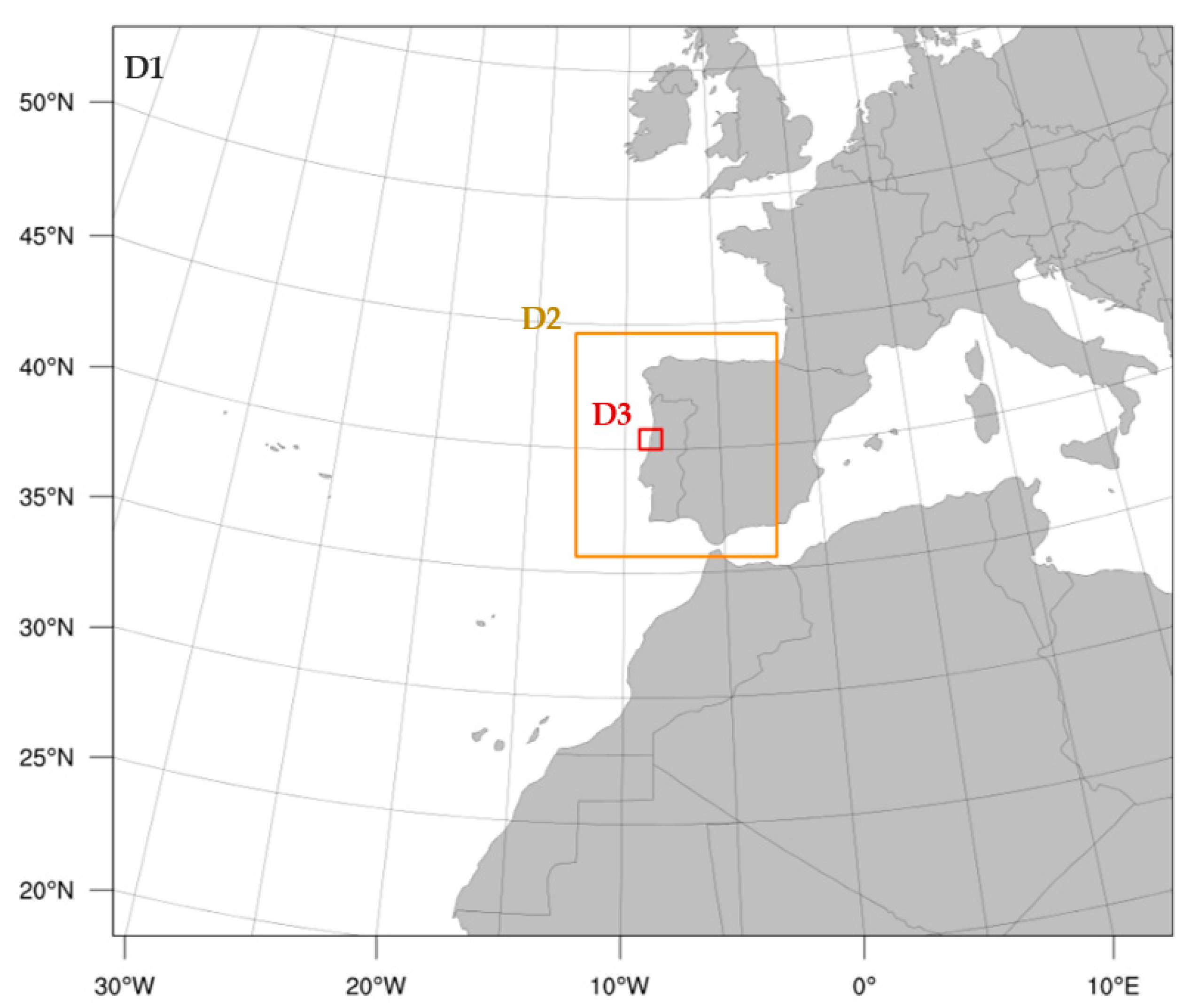
For this study, the model setup includes three nested domains, run in two-way mode, covering a large part of Europe and North Africa (D1, background domain), through a regional domain centred over Portugal (D2) to a Portuguese region (D3, inner domain) with horizontal grid resolutions of 25, 5, and 1 km, respectively (Figure 1). However, since the urban scale is the focus of this research, only NO2 results from domains 2 and 3 were analysed and compared. To solve the vertical structure of the atmosphere, 29 vertical levels extending up to 50 hPa were considered, with the lowest level at approximately 28 m above the surface.
Concerning the main physical and chemical model parametrisations, the following were adopted for the simulations: RADM2 (Regional Acid Deposition Model, second generation) chemical mechanism, MADE/SORGAM (Modal Aerosol Dynamics Model for Europe/Secondary Organic Aerosol Model) aerosol module, Fast-J photolysis, RRTMG (Rapid Radiative Transfer Model for General Circulation Models) short-wave/long-wave radiation schemes, and aerosol–radiation feedback were turned on. Other options and further details are presented in Silveira et al. [12].
2.2. Land Cover
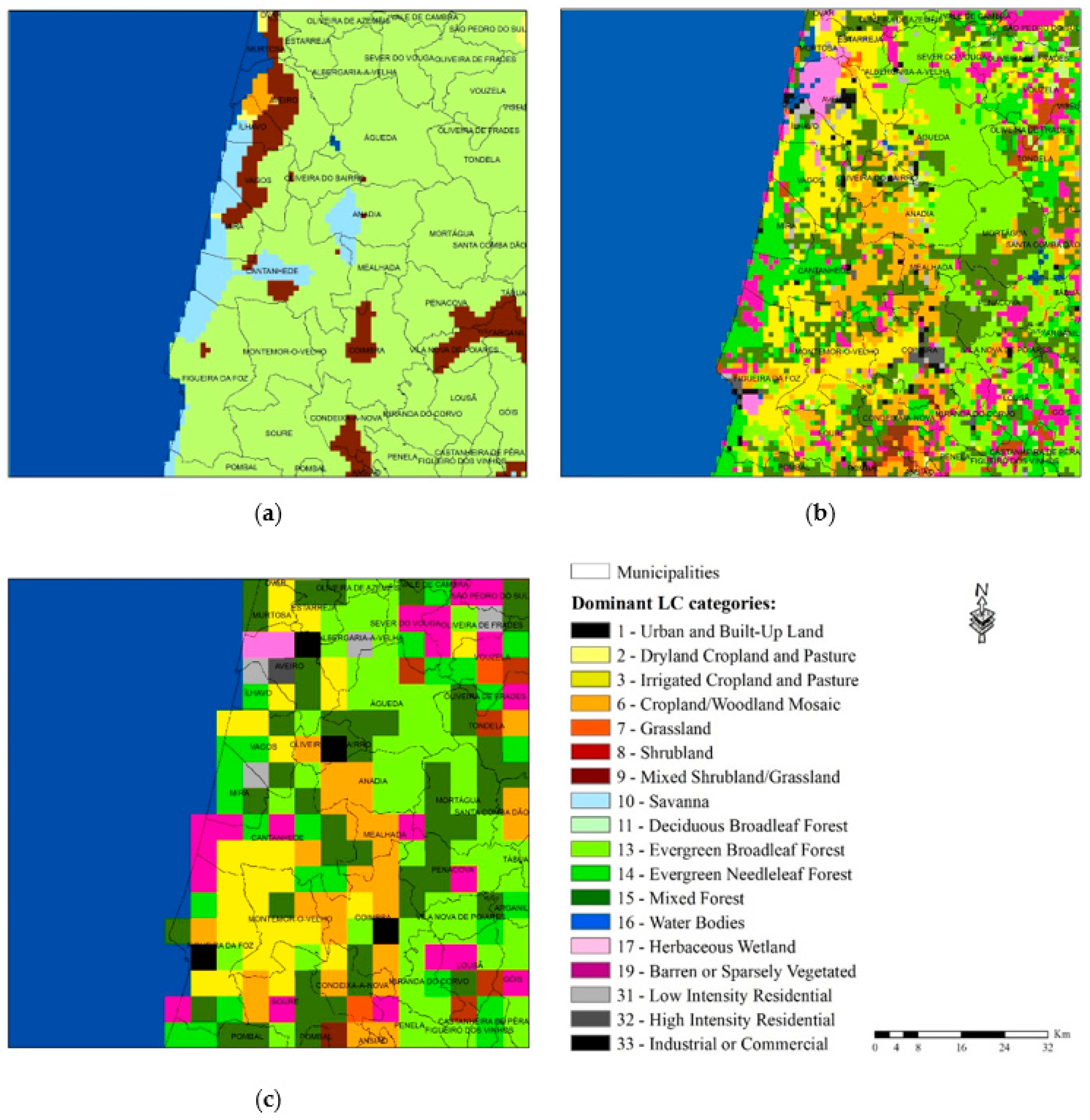
The LC arises as a prevailing driver of all interactions within the atmospheric boundary layer, directly influencing the Earth’s energy budget, and emission and deposition rates of air pollutants [26,27,33]. Given that preponderance of the LC on physical and chemical processes occurs in the atmosphere, a preliminary analysis based on different LC distributions for assessing air quality impacts was previously performed using the same WRF-Chem setup [28]. The analysis, involving the 24-classes USGS database (2-min horizontal resolution) provided with the WRF-Chem package against a new 33-classes LC classification, showed that the USGS LC reproduces unrealistically the spatial pattern under the simulation grids, and tends to a higher underestimation of maximum air quality values compared to the new LC. In the case of primary air pollutants, such as NO2, these evidences are stronger in urban areas, with higher emissions and a greater weight in the spatial allocation of these emissions for the simulation grids. Accordingly, since many urban areas are not identified or are roughly represented through the USGS database (class 1 in D3—Figure 2a), a more homogeneous spatial pattern of atmospheric concentrations is expected. In turn, the new LC classification, which combines CLC (CORINE Land Cover) for Europe with greater accuracy and specific LC data for Portugal, enables enhanced LC representation and air pollution hotspot identification; hence, it is selected as input for the WRF-Chem simulations.
Methodologically, this new LC database was developed and implemented within the WRF-Chem as follows: (i) CLC and national LC data were integrated in GIS (geographic information systems) software and reclassified according to the new 33-classes USGS nomenclature following those previously suggested [34]; (ii) in the LC reclassification process, the inclusion of three different urban classes: low-intensity residential (class 31), high-intensity residential (class 32), and industrial or commercial (class 33) should be highlighted; and (iii) lastly, the resulting LC was processed to be directly ingested by the model considering 5000 and 100 m horizontal resolutions for CLC areas and Portugal, respectively.
Once the new LC database was successfully implemented, the outcome was interpolated for the simulation domains taking into account the dominant LC category in each grid cell. Focusing on domain 3 coverage, Figure 2b,c shows the resulting LC for 1 and 5 km grid resolutions. However, it should be noted that the interpolation from very high-resolution data to coarse grid cells leads to considerable losses of detail, not taking the best advantage of the relevance of these inputs. This advice is particularly useful for studies over urban areas, where adjusted urban parametrisations and higher input and output resolutions are essential to improve the modelling performance.
3. Impact of the LC and Grid Spacing on NO2 Concentrations
Following the methodological scheme described in the previous section, the WRF-Chem was applied for the period 24 December 2014 to 31 December 2015, on a daily basis and with hourly resolution, discarding the days of December 2014 as model spin up. The spatial variability and range of modelled NO2 concentrations from domains 2 and 3 are analysed and discussed in Section 3.1. To evaluate the modelling performance, measurements from the Portuguese air quality monitoring stations were used (Section 3.2).
Emphasis was given to annual and hourly NO2 values, in accordance with the time periods established for the WHO guidelines for human health protection [2] and for the limit values of the European Commission’s Ambient Air Quality Directive 2008/50/EC.
3.1. Comparative Analysis
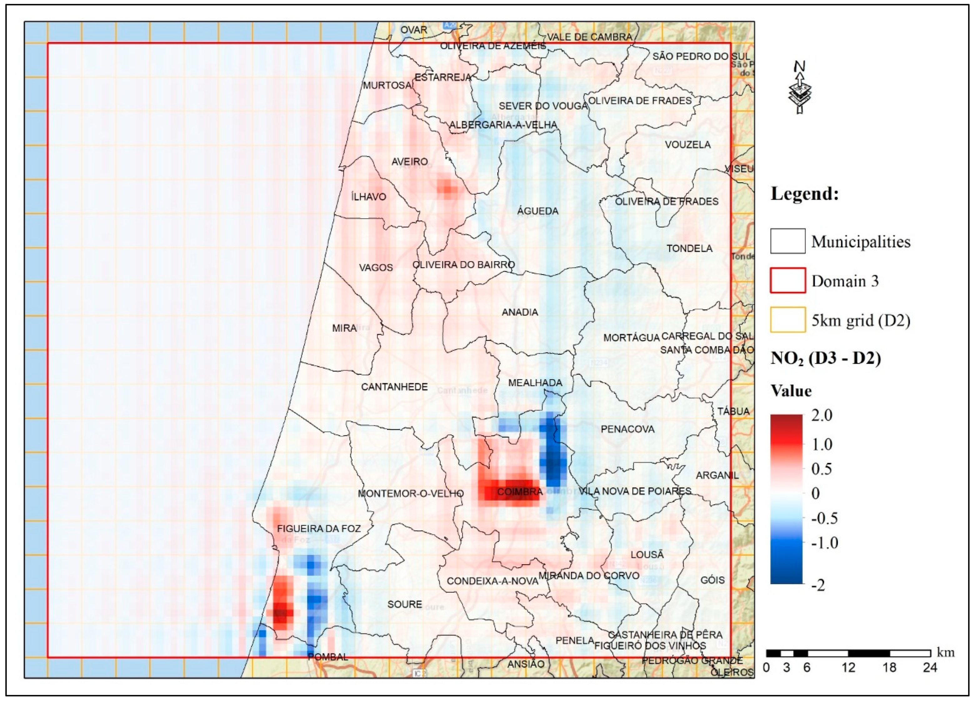
As a starting point to analyse the influence of the horizontal grid resolution on NO2 concentrations, annual mean spatial differences between D3 and the part of D2 that overlaps D3 (D3–D2 for each grid cell of D3) and its relationship with the new LC were quantified (Figure 3 and Figure 4).
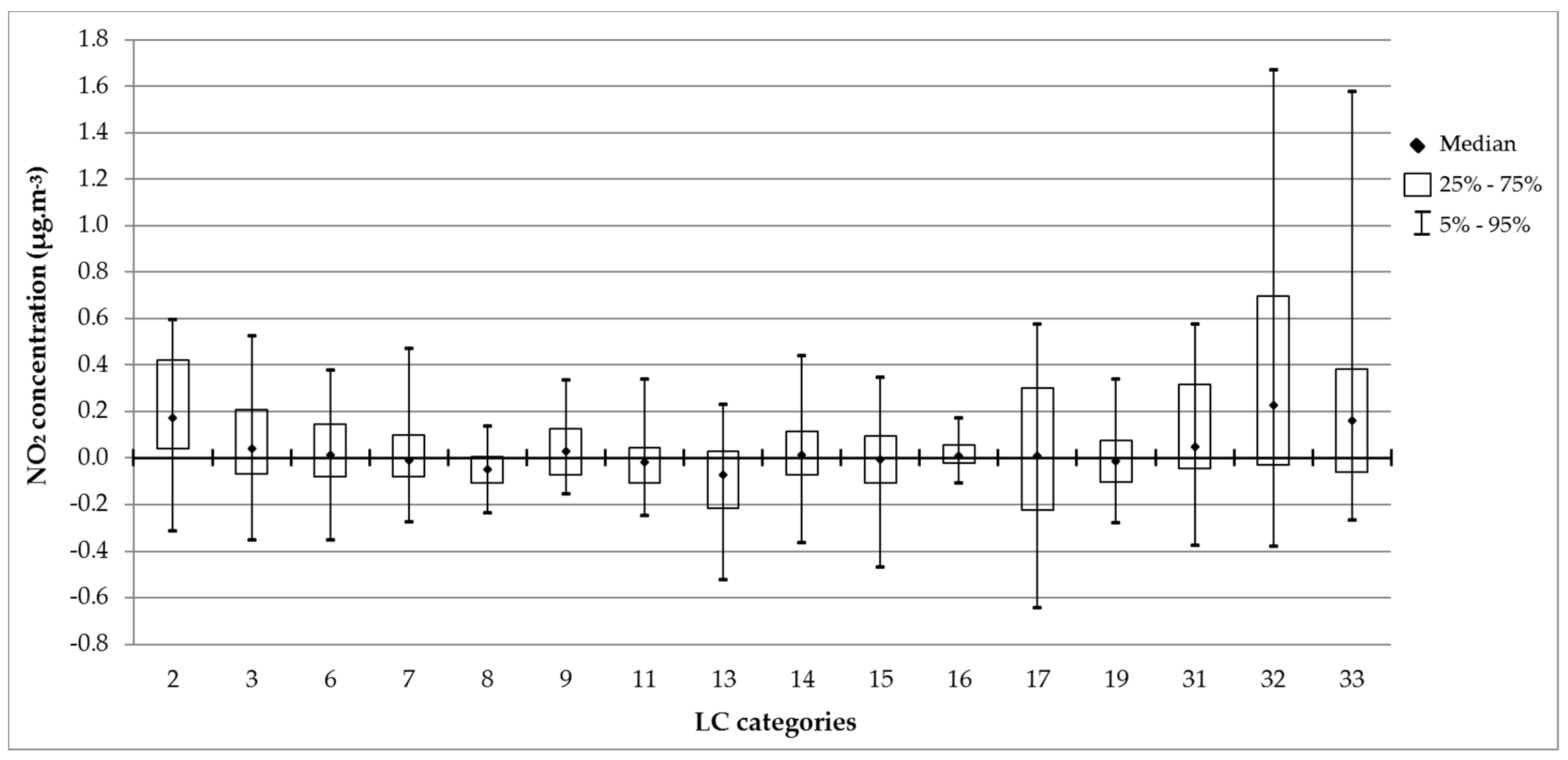
Looking at the spatial pattern of annual mean NO2 differences, the influence of the LC interpolation process under the simulation grids has a large impact, since the highest resolution from domain 3 solves the geographic location of the LC categories better and, consequently, an improved representation of the main emission sources and amount of emitted pollutant is expected. Hence, higher positive differences of NO2 concentrations (up to 2 µg·m−3) in pollution hotspots were found, which, to a certain extent of domain 2, are not properly captured, or even not identified. For the Aveiro and Figueira da Foz municipalities, more pronounced positive differences occur near the large industrial point sources, whereas for Coimbra, the resulting LC characterisation and associated road activity were the reason for raising the NO2 concentrations over domain 3. Supporting this information, Figure 4 shows the dominant LC categories for the D3 cells, where those identified as urban, mainly the categories 32 and 33 (high-intensity residential and industrial or commercial, respectively), contributed to higher NO2 values in relation to the D2 estimates. In contrast, for the surrounding area of these hotspots, higher concentrations were estimated for domain 2 (negative differences in Figure 3), probably due to the way the emissions were spatially distributed by the simulation grids, attributing a more uniform pattern to D2.
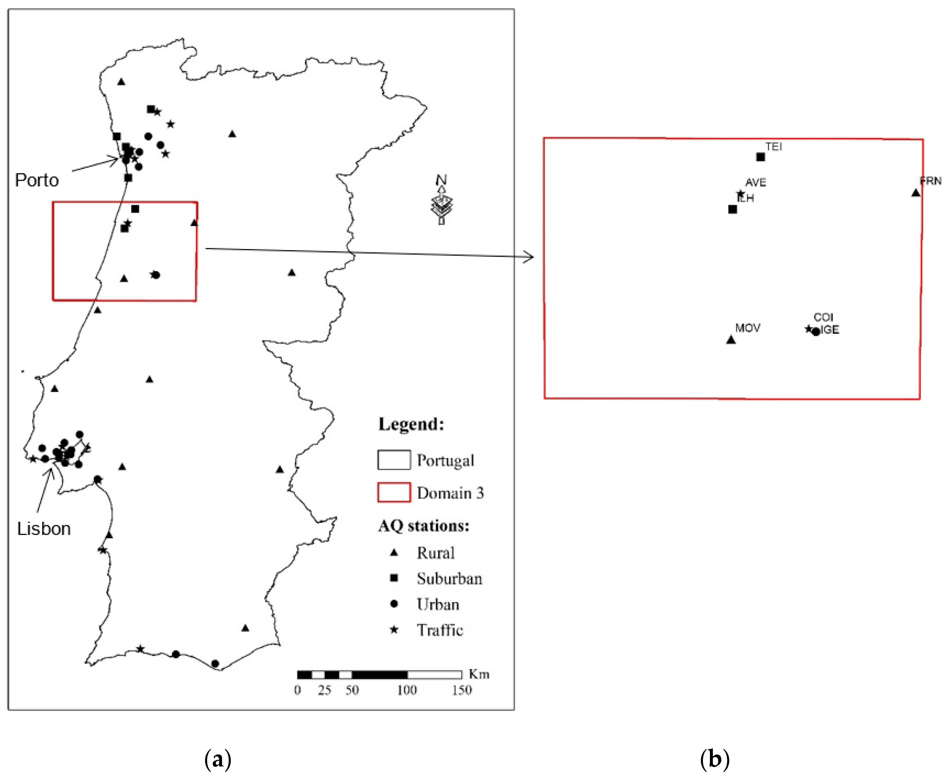
The predicted levels for D2 and D3 were compared with observations from air quality stations common to both simulation domains, taking into account the station type (Figure 5). In total, results for seven locations representing air quality stations (inside the red rectangle) are presented: 2 rural (FRN, MOV), 2 suburban (ILH, TEI), 1 urban (IGE), and 2 traffic (AVE, COI).
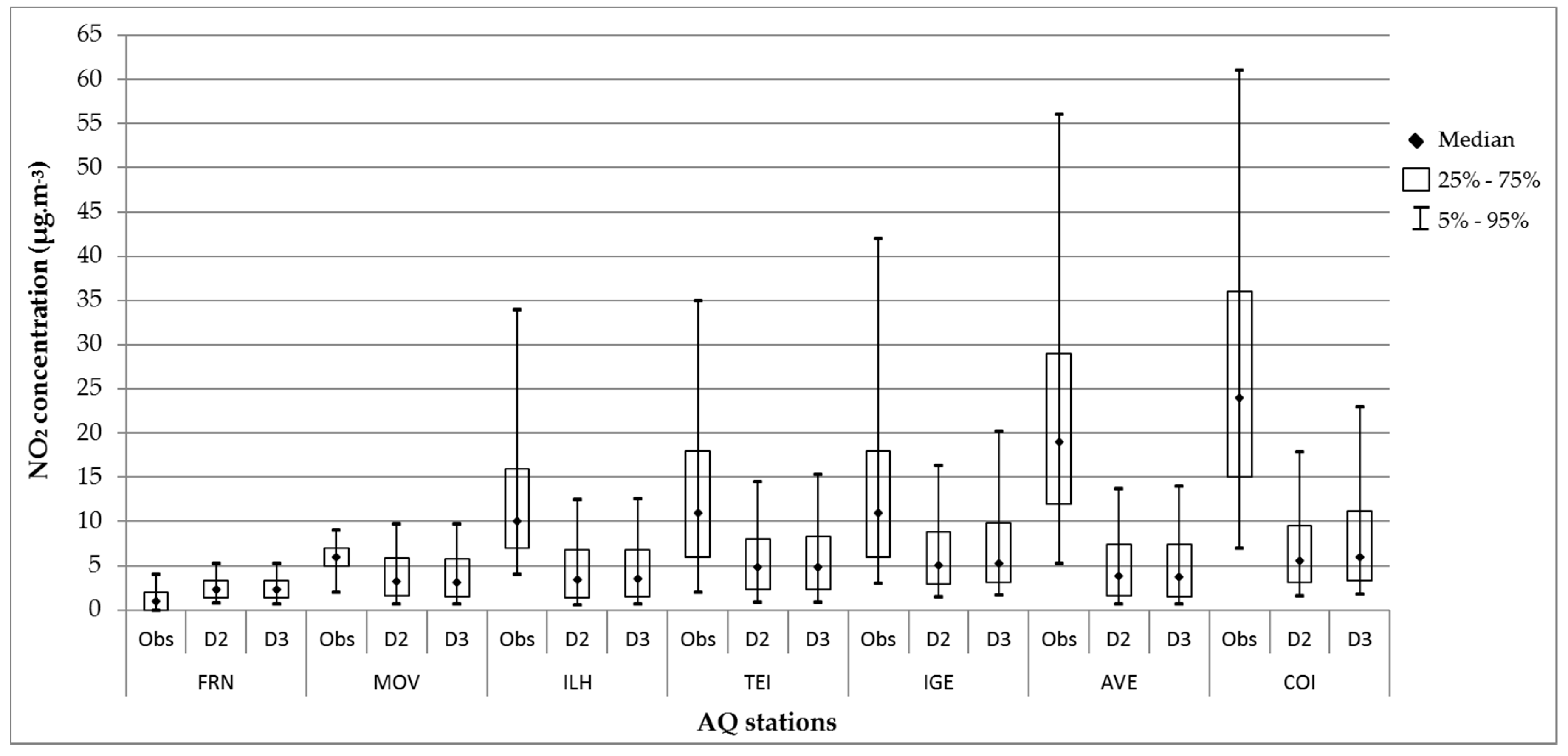
Figure 6 shows the median and some percentiles calculated for the hourly observed and modelled NO2 concentrations at these monitoring sites. Good agreement between observations and estimates was obtained in background rural stations (FRN, MOV), since these are normally located on quite homogeneous areas with limited and well-identified emission sources, which favours the numerical resolution of all processes occurring within the atmospheric boundary layer. In turn, as expected, highest measured values were recorded in traffic stations (AVE, COI), due to the intense road activity and its significant contribution to urban NO2 pollution.
The model is unable to reproduce the magnitude of the higher values, because despite the reasonable grid resolutions to portray urban areas, in particular of domain 3 (1 km), the EI used has a resolution (approximately 10 km) which does not allow for solving urban-scale air pollution patterns. The low resolution of the EI and its use in all simulation domains, contributed to the relatively small differences between D2 and D3. Nevertheless, there are other factors that could explain the variability of the modelled data and their underestimation, such as smoothing of areas with complex terrain, omission/underestimation of emission sources, and poorly reproduced meteorological processes. When comparing the results of traffic stations with the other typologies, differences between measured and modelled data tend to decrease substantially, demonstrating that the traffic-related NO2 emissions used for simulating air quality over urban areas with high traffic activity are clearly underestimated. At this scale, specific modelling tools and detailed characterisation of the local emission sources and urban geometry are required.
3.2. Model Evaluation
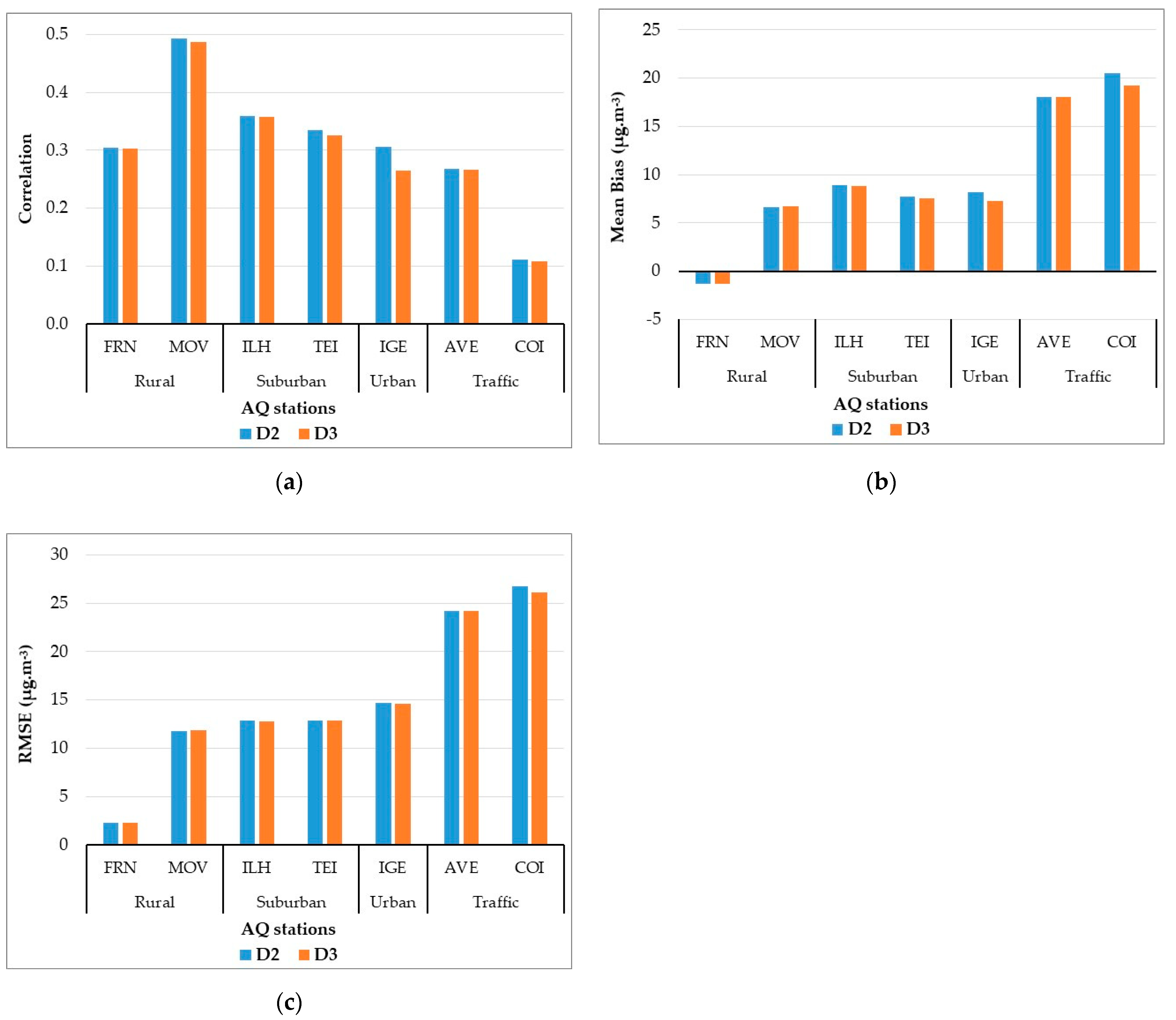
For a more comprehensive analysis of the agreement of WRF-Chem results with observed values, the model performance for the Portuguese air quality monitoring stations common to the D2 and D3 domains (Figure 5b) and for the year 2015 was evaluated, considering the following statistical metrics: Pearson´s correlation coefficient, mean bias, and root mean square error (RMSE) (Figure 7). Appendix A shows the equations used.
As expected, worst performance was found in traffic stations, with lower correlations and higher biases and RMSE. This model behaviour can be largely explained by the geographic location of these stations, since they are strategically positioned over urban street canyons with high traffic activity, and due to the low resolution of the EI used in all simulation domains, which contributed to a poor characterisation of the emission sources, mainly for urban/local-scale modelling purposes. In turn, this limited representativeness of the EI, associated to emissions evenly distributed in space and more simplified terrain features were the reason for the best estimates on rural areas, leading to the highest correlations and lowest biases and RMSE. Furthermore, the best agreement in rural stations can also be justified through the model’s numerical solving capabilities, which favour the simplified representation of the atmospheric processes, given the homogeneity and large distance from the main pollution sources that are typically associated to rural areas.
Comparing the modelled results for the sites common to both domains, the increase in the horizontal grid resolution from 5 km (D2) to 1 km (D3) did not greatly impact the model performance, despite the influence of the detailed LC in the spatial allocation of emissions. However, mean bias and RMSE tend to decrease with the increasing resolution, while a slightly higher correlation was obtained for the lower resolution.
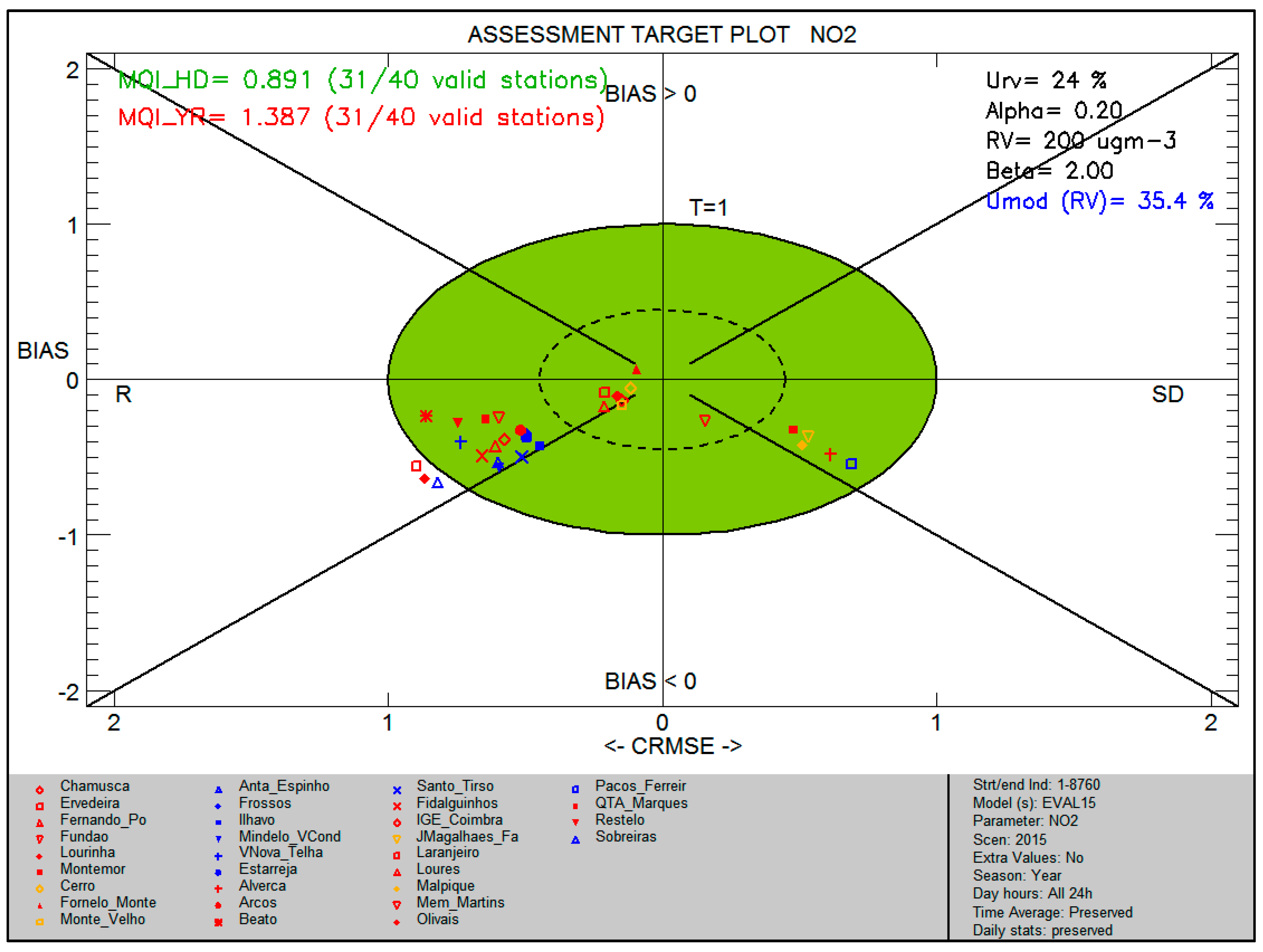
With the purpose of assessing the quality level of these estimates for policy support, the normalised target diagram using the Delta Tool was constructed (Figure 8) based on all Portuguese background air quality stations, identified as rural, suburban, and urban, as shown in Figure 5a. The diagram illustrates whether the model quality objectives (MQO) proposed in the Air Quality Directive (2008/50/EC) are fulfilled for at least 90% of the available stations. This approach consists of calculating the modelling quality indicator (MQI) associated with each station, which should be less than or equal to 1 (circle area) in order to meet the MQO. More details on Delta Tool can be found in Thunis et al. [35].
Statistics for the Portuguese background stations with more than 75% of data availability (31 out of 40) were produced, considering hourly series of modelled (D2) and observed NO2 concentrations. Instead of the mean bias and RMSE, the Delta Tool works with normalised BIAS and centred RMSE (see Appendix A for the equations). For the valid stations, an acceptable quality level based on hourly modelled values was obtained (MQI_HD of 0.891), but it failed when annual average NO2 concentrations were compared (MQI_YR of 1.387), due to the weaker performance verified for urban and suburban stations, as already shown in Figure 7. This can happen because different formulations are used for obtaining the hourly (MQI_HD) and yearly (MQI_YR) Modelling Quality Indicator. According to the guidance for the Delta Tool application [36], the difference between the two indicators is related to the autocorrelation in both the monitoring data and the model results, and the way the autocorrelations affect the uncertainty of the annual averaged values. The MQI_HD results from a ratio between the RMSE and a value representative of the maximum allowed measurement uncertainty, whereas the MQI_YR considers the difference of the yearly mean bias of modelled and measured concentrations normalised by the uncertainty of the measured mean concentration. On the other hand, on an hourly basis, considering multiple modelled–measured pairs could contribute to smoothing the differences. Nevertheless, the NO2 results for these MQI (MQI_HD < MQI_YR) are in accordance with other studies (e.g., [37,38]).
Therefore, the performance criteria for the target indicator are fulfilled in hourly estimates, and the following conditions for the stations are ensured:
- Normalised bias and centred RMSE (CRMSE) are less or equal to 1;
- Hourly modelled and observed data are positively correlated;
- Model uncertainty (Umod RV) of 35.4% is below the MQO´s uncertainty for ambient air quality assessment (50% for hourly NO2 data).
Overall, the model evaluation for NO2 concentrations is within the range of other research studies performed over regions with similar environmental conditions and by testing different combinations of inputs and physical and chemical model parametrisations [17,39,40,41,42].
Focusing on the aspects addressed in this study, the refinement of the LC and grid resolution contributes to a better spatial pattern of pollutant concentrations, namely over urban and industrial areas (Figure 3 and Figure 4), due to better allocation of emissions and thus better reproduction of NO2 hotspots. This improvement is confirmed by the validation results, which indicate slight increases of the calculated performance statistical indicators (Figure 6 and Figure 7). Therefore, modelling results are largely dependent on the spatial distribution of the system inputs and the statistical performance varies with the location/typology of the monitoring stations.
4. Conclusions
Air quality modelling over different nested domains is a current practice for assessing air pollutant concentrations at multiple spatial scales. However, choosing the appropriate domain resolutions is a challenging issue concerning both efficiency and accuracy of the predictions. Limited spatial resolution produces systematic errors in the model simulations, while finer resolution adds computational costs and may not be practical for operational air pollution forecasts. Moreover, increased spatial resolutions pose additional challenges concerning the required input data (e.g., LC, emissions), which may not be available to support fine resolutions, or the numerical limitations of the models themselves.
In this study, the impact of two nested high-resolution simulation domains focused on Portugal (D2 and D3, with 5 and 1 km horizontal grid resolutions) and on ambient NO2 concentrations, was investigated by applying the online WRF-Chem model for a whole year (2015). Taking advantage of this annual simulation at high resolutions, the combined effect of the grid spacing with a very detailed LC database was also analysed, given the LC influence on the atmospheric dynamics and spatial allocation of anthropogenic emissions under the simulation grids. To better understand the spatial fluctuations of NO2 concentrations, a model evaluation was performed by station typology. The following findings are noteworthy:
- Urban LC categories interpolated for the D3 enhanced pollution hotspots, with higher values (of up to 2 µg·m−3) in relation to D2, are probably due to the way the emissions were spatially distributed by the simulation grids;
- Small differences were found between D2 and D3 estimates, as a result of the low resolution of EI and its use in all simulation domains;
- Accordingly, the increase in horizontal resolution did not considerably help to improve model performance, with slightly smaller mean bias and RMSE for higher resolution, and slightly higher correlation values for lower resolution;
- The worst model performance obtained for traffic air quality stations (lower correlations and higher biases and RMSE) demonstrates the larger difficulty of this type of model and the configurations used to accurately reproduce air pollution levels at these sites;
- For policy support, the model quality objectives examining the hourly D2 results were fulfilled (MQO less than 1);
- Balancing the computational costs involved with the overall model performance, downscaling from 5 to 1 km grid resolution was not justified.
Overall, notwithstanding the poor improvement of the modelling performance shown by the comparison between observed and modelled values obtained for D2 and D3, the higher resolution of the simulation setup implied a better spatial allocation of land use, and therefore urban and industrial areas (Figure 2, LC categories 31–33) were better represented and simulated when capturing higher NO2 values. In fact, the effects of the LC interpolation process under the simulation grids had a considerable impact, since the highest resolution from D3 better solved the geographic location of the LC categories and, consequently, an improved representation of the main emission sources and amount of emitted pollutant was achieved.
However, even with these refinements, the main point from the results obtained is that increasing the spatial resolution of the model setup is not always an added value. This has to be accompanied by more detailed LC data and consequently by a better top-down, and if possible a mixed emission inventory approach. The use of other types of data sources (e.g., satellite data or road traffic or population dynamics-based proxies) could help on these more detailed input data, and should be explored when 1 km resolution and hourly simulations are projected.
In summary, for a CTM application down to 1 km horizontal resolution, an improved representation of the spatial and temporal variability of emissions under the simulation grids, together with the adjustment of model parametrisations according to the case study are required. Nevertheless, whenever modelling tools are used for multiscale and long-term air quality assessment purposes, prior planning, including proper characterisation of the study domains, selection of the modelling system to be used, how to couple the models with nesting capabilities (i.e., include feedbacks among the simulation domains), search/preparation of required input data, and evaluation of extreme weather events, is essential to improve both the understanding of atmospheric phenomena at different scales and the modelling performance. To complement this type of modelling studies, the use of satellite products is increasingly widespread by providing long-term data for wider areas [43,44].
The two main messages of this work to the scientific community rely on the importance of: (i) assessing the air quality in urban areas following a multiscale approach, for instance, by using nesting capabilities of models; and (ii) using detailed LC databases to improve the detail and consequently the robustness of gridded emissions.
Author Contributions
Conceptualisation, C.S., J.F. and A.I.M.; methodology, C.S.; software, P.T. and G.C.; formal analysis, C.S. and J.F.; investigation, C.S.; writing—original draft preparation, C.S.; writing—review and editing, C.S., J.F., A.I.M., P.T. and G.C.; supervision, J.F. and A.I.M. All authors have read and agreed to the published version of the manuscript.
Funding
The authors are grateful to the Foundation for Science and Technology (FCT, Portugal) for financial support by national funds FCT/MCTES to CIMO (UIDB/00690/2020), SusTEC (LA/P/0007/2020) and CESAM (UIDP/50017/2020+UIDB/50017/2020+ LA/P/0094/2020), and for the contract granted to Joana Ferreira (2020.00622.CEECIND). Thanks are also due for financial support to OleaChain project “Skills for sustainability and innovation in the value chain of traditional olive groves in the Northern Interior of Portugal” (NORTE-06-3559-FSE-000188).
Institutional Review Board Statement
Not applicable.
Informed Consent Statement
Not applicable.
Data Availability Statement
Not applicable.
Conflicts of Interest
The authors declare no conflict of interest.
Appendix A. Statistical Metrics
Pearson´s Correlation Coefficient (r):
Mean Bias (MBIAS):
Root Mean Square Error (RMSE):
Normalised Bias (NBIAS):
Centred RMSE (CRMSE):
where: Oi—observed values; Mi—modelled values; i—number (rank) between 1 and n; n—total number of observed or modelled values.
References
- WHO. Ambient (Outdoor) Air Pollution. Available online: https://www.who.int/news-room/fact-sheets/detail/ambient-(outdoor)-air-quality-and-health (accessed on 29 December 2021).
- WHO. WHO Global Air Quality Guidelines: Particulate Matter (PM2.5 and PM10), Ozone, Nitrogen Dioxide, Sulfur Dioxide and Carbon Monoxide; WHO: Geneva, Switzerland, 2021. [Google Scholar]
- EEA. Air Quality in Europe—2019 Report; European Environment Agency: Copenhagen, Denmark, 2019; ISBN 978-92-9480-088-6. [Google Scholar]
- Sundvor, I.; Castell Balaguer, N.; Viana, M.; Querol, X.; Reche, C.; Amato, F.; Mellios, G.; Guerreiro, C. Road Traffic’s Contribution to Air Quality in European Cities; ETC/ACM: Bilthoven, The Netherlands, 2012. [Google Scholar]
- Russo, A.; Trigo, R.M.; Martins, H.; Mendes, M.T. NO2, PM10 and O3 urban concentrations and its association with circulation weather types in Portugal. Atmos. Environ. 2014, 89, 768–785. [Google Scholar] [CrossRef]
- Silveira, C.; Ferreira, J.; Miranda, A.I. The challenges of air quality modelling when crossing multiple spatial scales. Air Qual. Atmos. Health 2019, 12, 1003–1017. [Google Scholar] [CrossRef]
- Thunis, P.; Miranda, A.; Baldasano, J.M.; Blond, N.; Douros, J.; Graff, A.; Janssen, S.; Juda-Rezler, K.; Karvosenoja, N.; Maffeis, G.; et al. Overview of current regional and local scale air quality modelling practices: Assessment and planning tools in the EU. Environ. Sci. Policy 2016, 65, 13–21. [Google Scholar] [CrossRef]
- Miranda, A.; Silveira, C.; Ferreira, J.; Monteiro, A.; Lopes, D.; Relvas, H.; Borrego, C.; Roebeling, P. Current air quality plans in Europe designed to support air quality management policies. Atmos. Pollut. Res. 2015, 6, 434–443. [Google Scholar] [CrossRef] [Green Version]
- Borrego, C.; Monteiro, A.; Sá, E.; Carvalho, A.; Coelho, D.; Dias, D.; Miranda, A.I. Reducing NO2 Pollution over Urban Areas: Air Quality Modelling as a Fundamental Management Tool. Water Air Soil Pollut. 2012, 223, 5307–5320. [Google Scholar] [CrossRef]
- Grell, G.A.; Peckham, S.E.; Schmitz, R.; McKeen, S.A.; Frost, G.; Skamarock, W.C.; Eder, B. Fully coupled “online” chemistry within the WRF model. Atmos. Environ. 2005, 39, 6957–6975. [Google Scholar] [CrossRef]
- Crippa, P.; Sullivan, R.C.; Thota, A.; Pryor, S.C. The impact of resolution on meteorological, chemical and aerosol properties in regional simulations with WRF-Chem. Atmos. Chem. Phys. 2017, 17, 1511–1528. [Google Scholar] [CrossRef] [Green Version]
- Silveira, C.; Martins, A.; Gouveia, S.; Scotto, M.; Miranda, A.I.; Monteiro, A. The Role of the Atmospheric Aerosol in Weather Forecasts for the Iberian Peninsula: Investigating the Direct Effects Using the WRF-Chem Model. Atmosphere 2021, 12, 288. [Google Scholar] [CrossRef]
- Schaap, M.; Cuvelier, C.; Hendriks, C.; Bessagnet, B.; Baldasano, J.M.; Colette, A.; Thunis, P.; Karam, D.; Fagerli, H.; Graff, A.; et al. Performance of European chemistry transport models as function of horizontal resolution. Atmos. Environ. 2015, 112, 90–105. [Google Scholar] [CrossRef] [Green Version]
- Borge, R.; Lumbreras, J.; Pérez, J.; de la Paz, D.; Vedrenne, M.; de Andrés, J.M.; Rodríguez, M.E. Emission inventories and modeling requirements for the development of air quality plans. Application to Madrid (Spain). Sci. Total Environ. 2014, 466–467, 809–819. [Google Scholar] [CrossRef] [Green Version]
- Ferreira, J.; Guevara, M.; Baldasano, J.M.; Tchepel, O.; Schaap, M.; Miranda, A.I.; Borrego, C. A comparative analysis of two highly spatially resolved European atmospheric emission inventories. Atmos. Environ. 2013, 75, 43–57. [Google Scholar] [CrossRef]
- Tie, X.; Brasseur, G.; Ying, Z. Impact of model resolution on chemical ozone formation in Mexico City: Application of the WRF-Chem model. Atmos. Chem. Phys. 2010, 10, 8983–8995. [Google Scholar] [CrossRef] [Green Version]
- Kuik, F.; Lauer, A.; Churkina, G.; Denier van der Gon, H.A.C.; Fenner, D.; Mar, K.A.; Butler, T.M. Air quality modelling in the Berlin–Brandenburg region using WRF-Chem v3.7.1: Sensitivity to resolution of model grid and input data. Geosci. Model Dev. 2016, 9, 4339–4363. [Google Scholar] [CrossRef] [Green Version]
- JRC—Joint Research Centre. TNO_MACC-III Inventory—Europa.eu. Available online: https://aqm.jrc.ec.europa.eu/fairmode/document/event/presentation/20150624-Aveiro/WG3/WG3 Kuenen.pdf (accessed on 29 December 2021).
- Kuenen, J.J.P.; Visschedijk, A.J.H.; Jozwicka, M.; van Der Gon, H.A.C.D. TNO-MACC-II emission inventory; A multi-year (2003-2009) consistent high-resolution European emission inventory for air quality modelling. Atmos. Chem. Phys. 2014, 14, 10963–10976. [Google Scholar] [CrossRef] [Green Version]
- Gego, E.; Hogrefe, C.; Kallos, G.; Voudouri, A.; Irwin, J.S.; Rao, S.T. Examination of model predictions at different horizontal grid resolutions. Environ. Fluid Mech. 2005, 5, 63–85. [Google Scholar] [CrossRef]
- Falasca, S.; Curci, G. High-resolution air quality modeling: Sensitivity tests to horizontal resolution and urban canopy with WRF-CHIMERE. Atmos. Environ. 2018, 187, 241–254. [Google Scholar] [CrossRef]
- Zhong, M.; Saikawa, E.; Liu, Y.; Naik, V.; Horowitz, L.W.; Takigawa, M.; Zhao, Y.; Lin, N.-H.; Stone, E.A. Air quality modeling with WRF-Chem v3.5 in East Asia: Sensitivity to emissions and evaluation of simulated air quality. Geosci. Model Dev. 2016, 9, 1201–1218. [Google Scholar] [CrossRef] [Green Version]
- Heald, C.L.; Spracklen, D.V. Land Use Change Impacts on Air Quality and Climate. Chem. Rev. 2015, 115, 4476–4496. [Google Scholar] [CrossRef] [Green Version]
- Lu, D.; Mao, W.; Yang, D.; Zhao, J.; Xu, J. Effects of land use and landscape pattern on PM2.5 in Yangtze River Delta, China. Atmos. Pollut. Res. 2018, 9, 705–713. [Google Scholar] [CrossRef]
- Sun, L.; Wei, J.; Duan, D.H.; Guo, Y.M.; Yang, D.X.; Jia, C.; Mi, X.T. Impact of Land-Use and Land-Cover Change on urban air quality in representative cities of China. J. Atmos. Sol.-Terr. Phys. 2016, 142, 43–54. [Google Scholar] [CrossRef]
- Wu, S.; Mickley, L.J.; Kaplan, J.O.; Jacob, D.J. Impacts of changes in land use and land cover on atmospheric chemistry and air quality over the 21st century. Atmos. Chem. Phys. 2012, 12, 1597–1609. [Google Scholar] [CrossRef] [Green Version]
- Xu, G.; Jiao, L.; Zhao, S.; Yuan, M.; Li, X.; Han, Y.; Zhang, B.; Dong, T.; Xu, G.; Jiao, L.; et al. Examining the Impacts of Land Use on Air Quality from a Spatio-Temporal Perspective in Wuhan, China. Atmosphere 2016, 7, 62. [Google Scholar] [CrossRef] [Green Version]
- Silveira, C.; Ascenso, A.; Ferreira, J.; Miranda, A.I.; Tuccella, P.; Curci, G. Influence of a High-Resolution Land Cover Classification on Air Quality Modelling. Int. J. Environ. Ecol. Eng. 2018, 12, 563–571. [Google Scholar] [CrossRef]
- Zou, B.; Xu, S.; Sternberg, T.; Fang, X.; Zou, B.; Xu, S.; Sternberg, T.; Fang, X. Effect of Land Use and Cover Change on Air Quality in Urban Sprawl. Sustainability 2016, 8, 677. [Google Scholar] [CrossRef] [Green Version]
- Tao, Z.; Santanello, J.A.; Chin, M.; Zhou, S.; Tan, Q.; Kemp, E.M.; Peters-Lidard, C.D. Effect of land cover on atmospheric processes and air quality over the continental United States-a NASA Unified WRF (NU-WRF) model study. Atmos. Chem. Phys. 2013, 13, 6207–6226. [Google Scholar] [CrossRef] [Green Version]
- Sun, W.; Liu, Z.; Zhang, Y.; Xu, W.; Lv, X.; Liu, Y.; Lyu, H.; Li, X.; Xiao, J.; Ma, F. Study on Land-use Changes and Their Impacts on Air Pollution in Chengdu. Atmosphere 2019, 11, 42. [Google Scholar] [CrossRef] [Green Version]
- Fast, J.D.; Gustafson, W.I.; Easter, R.C.; Zaveri, R.A.; Barnard, J.C.; Chapman, E.G.; Grell, G.A.; Peckham, S.E. Evolution of ozone, particulates, and aerosol direct radiative forcing in the vicinity of Houston using a fully coupled meteorology-chemistry-aerosol model. J. Geophys. Res. 2006, 111, D21305. [Google Scholar] [CrossRef]
- Jiménez-Esteve, B.; Udina, M.; Soler, M.R.; Pepin, N.; Miró, J.R. Land use and topography influence in a complex terrain area: A high resolution mesoscale modelling study over the Eastern Pyrenees using the WRF model. Atmos. Res. 2018, 202, 49–62. [Google Scholar] [CrossRef] [Green Version]
- Pineda, N.; Jorba, O.; Jorge, J.; Baldasano, J.M. Using NOAA AVHRR and SPOT VGT data to estimate surface parameters: Application to a mesoscale meteorological model. Int. J. Remote Sens. 2004, 25, 129–143. [Google Scholar] [CrossRef]
- Thunis, P.; Georgieva, E.; Pederzoli, A. A tool to evaluate air quality model performances in regulatory applications. Environ. Model. Softw. 2012, 38, 220–230. [Google Scholar] [CrossRef]
- Janssen, S.; Thunis, P. FAIRMODE Guidance Document on Modelling Quality Objectives and Benchmarking; European Union: Luxembourg, 2020. [Google Scholar]
- Karl, M.; Walker, S.E.; Solberg, S.; Ramacher, M.O.P. The Eulerian urban dispersion model EPISODE—Part 2: Extensions to the source dispersion and photochemistry for EPISODE-CityChem v1.2 and its application to the city of Hamburg. Geosci. Model Dev. 2019, 12, 3357–3399. [Google Scholar] [CrossRef] [Green Version]
- ENEA. AMS-MINNI National Air Quality Simulation on Italy for the Calendar Year 2015. Annual Air Quality Simulation of MINNI Atmospheric Modelling System: Results for the Calendar Year 2015 and Comparison with Observed Data; ENEA: Rome, Italy, 2020. [Google Scholar]
- Karlický, J.; Huszár, P.; Halenka, T. Validation of gas phase chemistry in the WRF-Chem model over Europe. Adv. Sci. Res. 2017, 14, 181–186. [Google Scholar] [CrossRef] [Green Version]
- Žabkar, R.; Honzak, L.; Skok, G.; Forkel, R.; Rakovec, J.; Ceglar, A.; Žagar, N. Evaluation of the high resolution WRF-Chem (v3.4.1) air quality forecast and its comparison with statistical ozone predictions. Geosci. Model Dev. 2015, 8, 2119–2137. [Google Scholar] [CrossRef] [Green Version]
- Tuccella, P.; Curci, G.; Visconti, G.; Bessagnet, B.; Menut, L.; Park, R.J. Modeling of gas and aerosol with WRF/Chem over Europe: Evaluation and sensitivity study. J. Geophys. Res. Atmos. 2012, 117, D03303. [Google Scholar] [CrossRef] [Green Version]
- Balzarini, A.; Pirovano, G.; Honzak, L.; Žabkar, R.; Curci, G.; Forkel, R.; Hirtl, M.; San José, R.; Tuccella, P.; Grell, G.A. WRF-Chem model sensitivity to chemical mechanisms choice in reconstructing aerosol optical properties. Atmos. Environ. 2015, 115, 604–619. [Google Scholar] [CrossRef]
- Mak, H.W.L.; Laughner, J.L.; Fung, J.C.H.; Zhu, Q.; Cohen, R.C. Improved Satellite Retrieval of Tropospheric NO2 Column Density via Updating of Air Mass Factor (AMF): Case Study of Southern China. Remote Sens. 2018, 10, 1789. [Google Scholar] [CrossRef] [Green Version]
- Xu, J.; Lindqvist, H.; Liu, Q.; Wang, K.; Wang, L. Estimating the spatial and temporal variability of the ground-level NO2 concentration in China during 2005–2019 based on satellite remote sensing. Atmos. Pollut. Res. 2021, 12, 57–67. [Google Scholar] [CrossRef]
Figure 1.
Nested simulation domains.

Figure 2.
Dominant LC categories mapped for domain 3 coverage resulting from interpolation under the simulation grids: (a) default USGS LC and (b) new LC for 1 km grid resolution; (c) new LC for 5 km grid resolution (D2 cut on D3 area).
Figure 2.
Dominant LC categories mapped for domain 3 coverage resulting from interpolation under the simulation grids: (a) default USGS LC and (b) new LC for 1 km grid resolution; (c) new LC for 5 km grid resolution (D2 cut on D3 area).

Figure 3.
Spatial distribution of the annual mean NO2 differences (µg·m−3) between D3 and D2.

Figure 4.
Annual mean NO2 differences (µg·m−3) between D3 and D2 grouped by dominant LC category. For the legend of LC categories, see Figure 2.
Figure 4.
Annual mean NO2 differences (µg·m−3) between D3 and D2 grouped by dominant LC category. For the legend of LC categories, see Figure 2.

Figure 5.
(a) Portuguese air quality monitoring network and (b) common stations to both simulation domains (D2 and D3) used for model validation.
Figure 5.
(a) Portuguese air quality monitoring network and (b) common stations to both simulation domains (D2 and D3) used for model validation.

Figure 6.
Statistics (median and percentiles) for the hourly NO2 concentrations (µg·m−3) observed (Obs) and modelled in domains D2 and D3.
Figure 6.
Statistics (median and percentiles) for the hourly NO2 concentrations (µg·m−3) observed (Obs) and modelled in domains D2 and D3.

Figure 7.
(a) Correlation, (b) mean bias, and (c) RMSE between the NO2 observations from Portuguese air quality monitoring stations and the modelled concentrations (µg·m−3) for domains D2 and D3.
Figure 7.
(a) Correlation, (b) mean bias, and (c) RMSE between the NO2 observations from Portuguese air quality monitoring stations and the modelled concentrations (µg·m−3) for domains D2 and D3.

Figure 8.
Target diagram for hourly NO2 concentrations considering Portuguese background air quality stations.
Figure 8.
Target diagram for hourly NO2 concentrations considering Portuguese background air quality stations.


Table 1.
Input datasets used in the numerical WRF-Chem simulations.
| Category | Subcategory | Source | Resolutions |
|---|---|---|---|
| Static data | Topography, soil properties, albedo | USGS | 2 arc-minute |
| Emissions | Anthropogenic | EMEP (for 2015) | 0.1° × 0.1° |
| Biogenic | MEGAN v2.04 | ||
| Initial and boundary conditions | Meteorological | ECMWF | 0.5° × 0.5°, every 6 h |
| Chemical | MOZART-4/GEOS-5 | 1.9° × 2.5°, every 6 h |
Acronyms: USGS—United States Geological Survey; EMEP—European Monitoring and Evaluation Programme; MEGAN—Model of Gases and Aerosols from Nature; ECMWF—European Centre for Medium-Range Weather Forecasts; MOZART-4/GEOS-5—Global Model for Ozone and Related Chemical Tracers.
Publisher’s Note: MDPI stays neutral with regard to jurisdictional claims in published maps and institutional affiliations. |
© 2022 by the authors. Licensee MDPI, Basel, Switzerland. This article is an open access article distributed under the terms and conditions of the Creative Commons Attribution (CC BY) license (https://creativecommons.org/licenses/by/4.0/).
Share and Cite
MDPI and ACS Style
Silveira, C.; Ferreira, J.; Tuccella, P.; Curci, G.; Miranda, A.I. Combined Effect of High-Resolution Land Cover and Grid Resolution on Surface NO2 Concentrations. Climate 2022, 10, 19. https://doi.org/10.3390/cli10020019
AMA Style
Silveira C, Ferreira J, Tuccella P, Curci G, Miranda AI. Combined Effect of High-Resolution Land Cover and Grid Resolution on Surface NO2 Concentrations. Climate. 2022; 10(2):19. https://doi.org/10.3390/cli10020019
Chicago/Turabian StyleSilveira, Carlos, Joana Ferreira, Paolo Tuccella, Gabriele Curci, and Ana I. Miranda. 2022. "Combined Effect of High-Resolution Land Cover and Grid Resolution on Surface NO2 Concentrations" Climate 10, no. 2: 19. https://doi.org/10.3390/cli10020019
Note that from the first issue of 2016, this journal uses article numbers instead of page numbers. See further details here.