
Methanol–Water Purification Control Using Multi-Loop PI Controllers Based on Linear Set Point and Disturbance Models


Department of Chemical Engineering, Faculty of Engineering, Universitas Indonesia, Depok 1642, Indonesia
*
Author to whom correspondence should be addressed.
ChemEngineering 2021, 5(4), 70; https://doi.org/10.3390/chemengineering5040070
Submission received: 9 September 2021
/
Revised: 9 October 2021
/
Accepted: 12 October 2021
/
Published: 20 October 2021
Abstract
:Dimethyl ether (DME), derived from methanol, has been issued as an alternative to diesel and LPG. This study will continue the research of an optimized process control design for DME purification plants, specifically the methanol purification process. This way, water can be separated, and the main product, methanol, can be recycled for DME synthesis. A setpoint-based linear model of a methanol–water purification system has been developed with four controlled variables (CV) with objectives to; maintain a separated liquid water stream in the bottom stage (Stage 30) of the distillation column for methanol–water separation at 11.22%, keep the purified liquid methanol at a condenser at 58.81 °C and 49.96% of level, and the last CV is the cooler in the distillate stream, to keep the purified methanol’s top product at 40.75 °C. To complete the model, a first order plus dead time (FOPDT) disturbance model is created against the inlet temperature and flow rate of the feed, the major cause of disturbances in the industry. Using a traditional proportional integral controller connected to each controlled variable, a multi-loop control system is formed with optimization and compared to the disturbance rejection of multivariable model predictive control (MMPC). The final improvement against the feed temperature and flow for CV1, CV2, CV3, and CV4 is shown by, respectively, Integral Absolute Error (IAE) values of 79.49%, 99.90%, 100%, and 99.99% and Integral Square Error (ISE) values of 97.1%, 100%, 99.99%, and 100%.
1. Introduction
In 2018, the energy consumption in Indonesia reached a total of 936.33 trillion barrels of oil equivalent (BOE), with 64.46 million BOE for LPG and 450.78 million BOE for fuel [1]. Energy demands and supply projections for 2019–2050 target induction stoves and DME utilization for liquefied petroleum gas (LPG) substitution. DME features easy volatility, no toxicity, no carcinogenicity, good water and alcohol solubility, and no pollution it is miscible with many resins and solvents. At ambient conditions, DME, similar to LPG, can be liquefied at moderate pressure. With a high cetane number, DME is clean-burning and sulfur-free, with extremely low particulates [2,3]. DME is derived from methanol from coal, natural gas, organic waste, and biomass [4]. Companies such as Topsoe, Mitsubishi Co., and Total have recently focused on promoting DME as a new and renewable fuel that can replace LPG and diesel. Solichin et al., (2011) [5] designed a DME purification plant suited and adjusted for Indonesia. In addition to the close market share, raw materials and auxiliary materials can be obtained in Indonesia, resulting in a reduced dependency on imported products. The manufacturing process starts with synthetic gas (CO2 and H2O) that is further synthesized into methanol and dehydrated into DME. The conversion from methanol to DME will still produce excess methanol and water, so they would be separated in a distillation column where the purified methanol is recycled to produce more DME [6,7,8]. This is different from what has been studied by Dyrda et al. [9], who used a membrane-based separation process to separate methanol and water to improve the performance of the fuel cell. In this research, a distillation column is used for separating methanol and water.
What is left is the optimization of this plant design. Process control is the integration of a mathematical model into an operating program [10] to optimize manufacturing, and its quality results in an improvement in safety standard profits [11]. The design of a system controller for the purification process of DME and methanol has been studied several times. A performance evaluation of the traditional proportional integral (PI) controller on DME and methanol purification was conducted by Wahid and Gunawan (2015) [12]. Wahid and Brillianto (2020) then developed a multiple input–multiple output (MIMO) process model with a single controller as the central brain (centralized controller) for the purification of methanol (methanol–water separation) in a DME plant [13]. The MIMO model created is based on the interaction of a controlled variable and how the changes to its manipulated variable affect other controlled variables. Each interaction is described with a linear first order plus dead time (FOPDT) model because a linear model offers simplicity and a reliable solution for system optimization.
This study aims to enhance the centralized control of the methanol purification process into a decentralized (multi-loop) control, in which each of manipulated variables has its controller, creating a multi-loop scheme rather than a single direct control of a multivariable process. A decentralized controller produces a higher result of stability from its faster and more accurate response compared to a centralized controller [14].
Multivariable control has been studied for decades, since nearly all processes would involve a simultaneous control on the production rate (flow), inventory (level and pressure), and process environment (temperature). There are three advantages of using multiple single-loop controllers. The first is that simple algorithms are easy to use, which helps when calculations are implemented with analog computing equipment, the second is that it is easy for plant operating personnel to understand the control structure (they only need to monitor the controlled variables and adjust its related manipulated variable), and the last is that the standard control designs are developed for the common unit. Although analysis and experience are required, multiloop designs will continue to be used extensively [11]. For this reason, the performance of multi-loop PI controllers and the tuning method of Big Log-Modulus Tuning has been studied and endorsed by Vu & Lee (2007), Biyanto et al., (2018), and M. Farsi (2015) [15,16,17].
Many process control designs and implementations can benefit from linear transfer function models created using empirical approaches. FOPDT models are suitable for process control analysis and design with dead time. The linear regression identification approach is more generic and may be used in industrial processes [11]. The examples of a linear model on common units are the 2 × 2 MIMO model by Wood-Berry, Vinante-Luyben, Wardle-Wood, and Ogunnaike-Ray for a distillation column. They utilize two controlled variables and two manipulated variables. Ogunnaike-Ray also created a 3 × 3 MIMO model, and a 4 × 4 MIMO model was created by Alatiqi. All of these were studied further by Huang et al. (2003) for their simplicity and implementation [18]. The Wood-Berry distillation column was then proposed using the fractional order PID (FOPID) controller and proved to be successful in terms of performance [19]. Other research conducted by Kalpana et al. (2017), Memon and Kalhoro (2021), and Alawad and Muter (2021) has proven the success of a multivariable PID controller [20,21,22]. However, they used an existing model. Here, this study develops a disturbance model, as was done by Ogunnaike and Ray (1979) on the Wood-Berry model (1973), which was originally only the SP model [23].
Since we already have the setpoint (SP) models by Wahid and Brillianto (2020) [13], the disturbance model will be created using the same method as the FOPDT model. The used FOPDT method ensures that the actual process is best represented. To make the controller more appropriate for factory conditions in real time, we added manual disturbance and adjusted the controller to be more responsive to the disturbance.
Dietrich et al.’s (2020) study about a DME plant for power concluded that the feed composition and temperature have a significant impact on the composition of the product, and this is because they are inconsistent and prone to be unstable after derivation from syntactic gas [24]. Thus, these two variable changes will be observed with the controlled variables of the process and then described with the FOPDT model. With a MIMO process model, a disturbance model, and an efficient PI control for each manipulated variable, a comprehensive and equipped multi-loop PI controller is created for the methanol purification process in the DME production plant.
2. Methods
2.1. Data Collection
The simulation of purification is made separately to reduce the variables that need to be controlled. The separation of methanol from water is based on the difference in boiling points: 64.7 °C and 100 °C, respectively. The data used were collected from Solichin et al.’s (2011) [5] studies on DME factory design. Table 1 and Table 2 below are the parameters for each unit.
2.2. Creating the Disturbance Model through System Identification
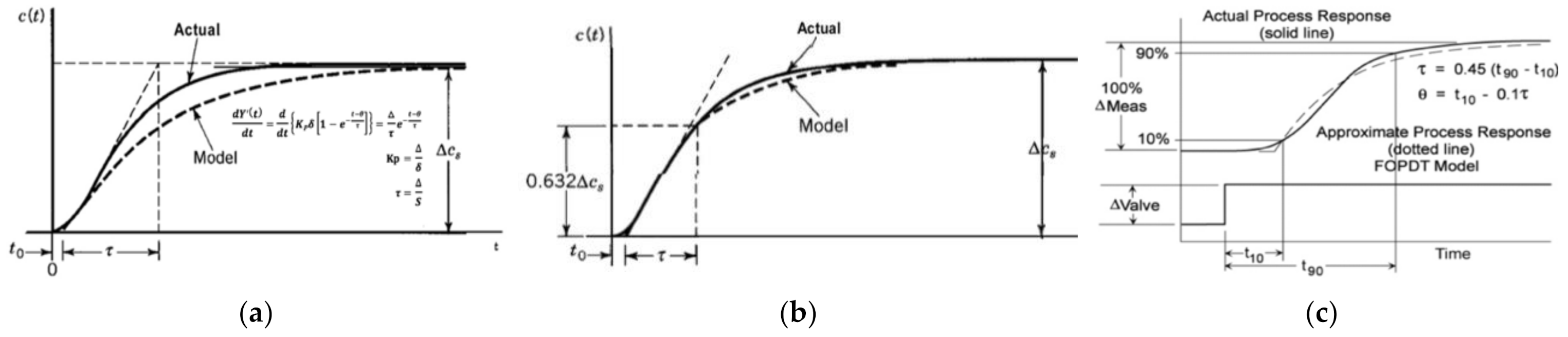
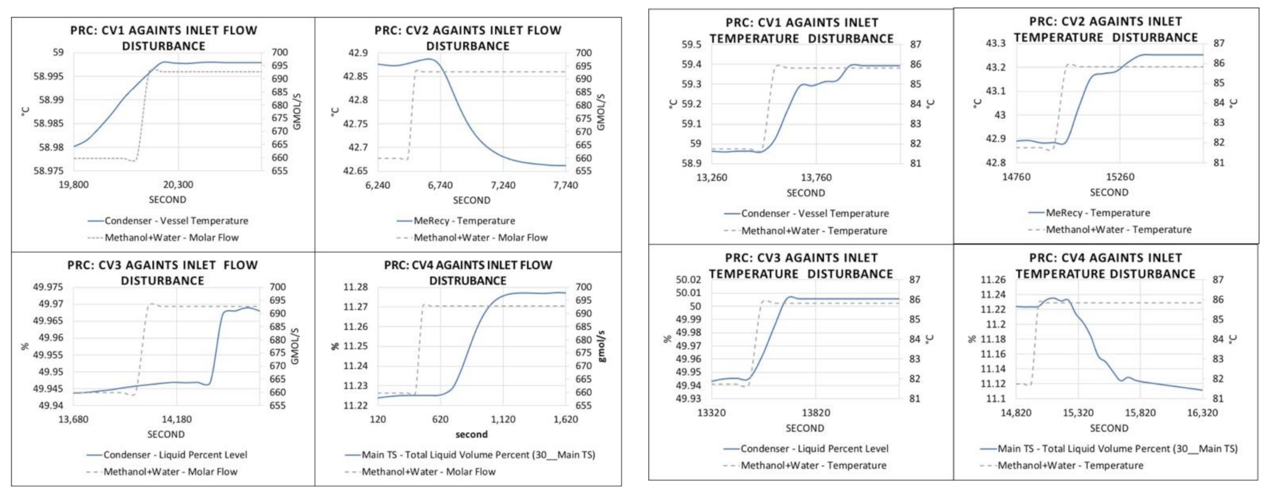
System identification is then conducted to create a dynamic system-based mathematical model based on the input and output signals of the system called a transfer function. Empirical models are designed completely using observational empirical evidence, data input, and data output from a dynamic system. A linear empirical dynamic model of a process is calculated using experimental data, one of which is to use step-response data. Interpretations may use Marlin’s (2000) process reaction curve (PRC) method [11]. Parameters of a PRC include the dead time (ϴ), the time constant (𝞃), the magnitude of the input shift (δ), the magnitude of the steady-state change in the output (Δ), and the overall slope (S). When measurement noise is considered, the model parameters can be precisely calculated. Deriving from the tangent line, the second method of the PRC by Smith (1972) resembles the closest actual process response, as pictured in Figure 2 below [24].
Thus, the parameters resulted will be used to create a transfer function of the first order plus dead time (FOPDT) method (Equation (4)).
2.3. Controller Pairing
The MIMO (multi-input–multi-output) method is a process control system that can manage process variables that communicate with a single controller at the same time [25]. A decentralized control system is a multivariable system where n inputs and n output variables are treated as n mono-variable systems. A decentralized control structure has certain advantages, such as design and hardware simplicity and ease of use [26].
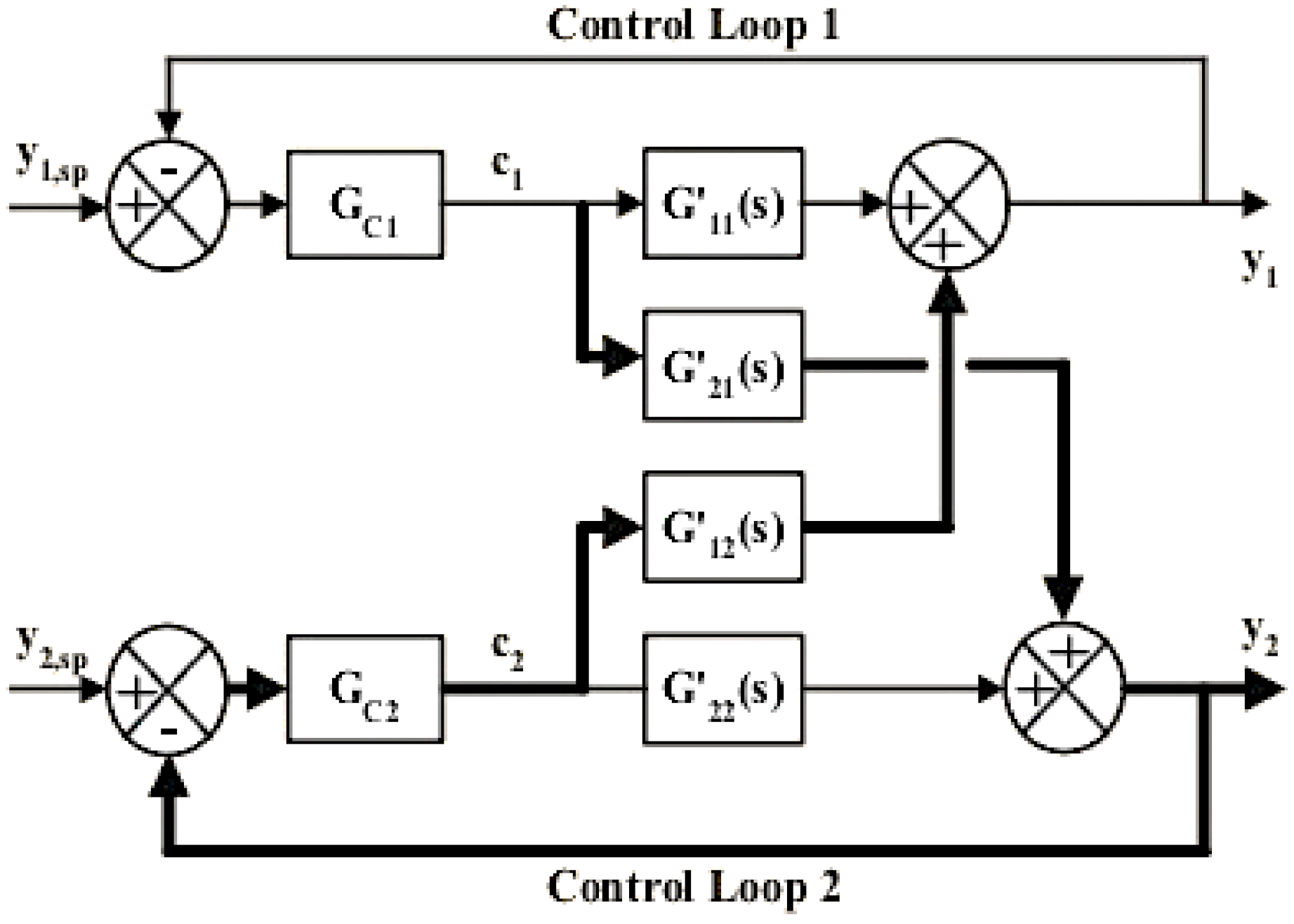
The motive for using a MIMO proportional integral controller for multi-loop control is its trouble-free configuration, straightforward tuning, and its ability to attain most of the estimated control objectives [27]. In multi-loop control, each manipulated variables (n) depend on a single controller (Gc) (Figure 3).
Equation (5) below is the purification 4 × 4 MIMO process model by Wahid and Brillianto (2020). The controlled variables include the condenser temperature (𝑇cond), the cooler output temperature (𝑇cooler), the condenser level (𝐿cond), and the column level (𝐿column). The manipulated variables are the condenser load (𝑄cond), the cooler load (𝑄cooler), the distillate flow rate (𝐹D), and the lower product flow rate (𝐹B) [13].
Control pairings themselves are chosen based on the process interactions, dynamic responses, and sensitivity to disturbance [14]. To find which control pairing works best, a relative gain array (RGA) (λ) is one way to decide (Equation (5)). Table 4 and Table 5 explain the interaction between the variables from their RGA.
where
Gp = process model; m = controlled variable;
Kp = process gain; n = manipulated variable;
Λ = RGA value.
2.4. Controller Tuning
Process interactions may include undesirable interactions between two or more control loops. The special characteristics of the proportional integral controller, however, are as follows:
- -
- There are changes in output if the error is not zero. Because of its design, even in small error situations, this controller will eradicate errors.
- -
- The reset time (𝜏i) ensures that the output returns to the set stage.
PI controllers are ineffective when processes with loads shift very rapidly and processes have a substantial lag between corrective actions and the resulting actions. However, since the DME plant does not require significant changes, the PI controller (Equation (6)) is used. Major load changes and significant variations at the setpoint can be properly controlled by the PI without prolonged oscillation or a permanent offset. After the disruption has occurred, it is easily returned to its proper state.
Controller tuning is used for achieving closed-loop stability. A way to tune decentralized PI controllers is through the biggest long-modulus tuning (BLT) method. This method idea is to tune individual interacting loops and then to de-tune all the loops together with a common factor (F) such that the overall system is stable and gives acceptable load disturbance rejection responses. The BLT method steps are as follows:
- Calculating initial PI parameter values;
- BLT de-tuning:
- Assume factor F with a typical range of 1.5 < F < 4;
- Calculate new values of the controller’s parameter, where the detune controller gain is Kci, and the detune reset time is 𝛕ii:
- Determine the log modulus function (Lc) using a multivariable Nyquist plot (W):
- Reassume the F factor until the bode plot of W is stable, indicators are stated in Table 6 below.
2.5. Performance Evaluation
For each process system, the sample to be taken and evaluated in this study is the CV graph monitored through setpoint tracking and disturbance rejection until the stable condition is reached again. Analysis was conducted using the performance parameters of the Integral Absolute Error (IAE) and the Integral Square Error (ISE).
The IAE is the absolute area of the difference between the area of the setpoint graph and the area of the controlled variable (CV) response graph. This makes the IAE easy to analyze. Meanwhile, the ISE value can be calculated by first squaring the existing data. IAE is better at detecting minor errors. This is because, when the value is smaller than 1, the ISE value will be smaller. IAE also does not have an error with negative values. For long-duration transients, ITAE (Integral of Time-Weighted Absolute Error) would perform best to penalize their deviations. However, the IAE and ISE perform better to correct errors precisely and with a fast response [11]. Since both hold time and deviation accountable, they are enough to underline the performance of a controller. The IAE and ISE can be used independently as a performance indicator of process control because the best IAE or ISE holds the best score [29]. Below are their equations.
3. Results and Discussion
3.1. Disturbance Model
The model is obtained using the first order plus dead time (FOPDT) approach and the step response method. CV and MV changes during response changes will produce a PRC, from which we derive a transfer function that will be used to tune the controller. The disturbances that have been identified in this system are the instability of temperature and flow rate in the distillation column. Therefore, the PRC that is made is the influence of the feed-in temperature and flow rate on the liquid level and temperature in the distillation column and its condenser.
The feed-in molar flow and the temperature are increased by 5% on a separate simulation from 659.8 gmol/s to 692.78 gmol/s and from 81.74 °C to 85.827 °C. The disturbance transfer function model derived from the PRC in Figure 4 is concluded in Table 7. The excess flow causes a rise in the T-103 Condenser’s temperature and level. The higher feed-in temperature must have caused the mixture to expand more, causing a lower level in Stage 30 due to a faster condensing and an increase in condenser level. The decreasing slope results in a negative process gain value.
Thus, the final disturbance model (Gd) for methanol–water separation in DME synthesis, with FF as the feed flow rate and TF as the feed temperature, is as shown below.
3.2. Controller Pairing
The pairing results from the methanol purification 4 × 4 MIMO process model by Wahid and Brillianto (2020) [13]. RGA analysis is CV2-MV2 and CV4-MV4, as shown as bold below, from the Matlab coding program.
| RGA11 = | RGA21 = | RGA31 = | RGA41 = |
| 0.2452 | 15.8404 | 265.6956 | 0.1637 |
| RGA12 = | RGA22 = | RGA32 = | RGA42 = |
| 0.0555 | 0.6979 | −4.7820 | 0.1538 |
| RGA13 = | RGA23 = | RGA33 = | RGA43 = |
| −0.7833 | −50.8558 | −851.0568 | 0.2304 |
| RGA14 = | RGA24 = | RGA34 = | RGA44 = |
| −0.0915 | −6.7712 | −111.6737 | 1.0274 |
CV1 was paired with MV1 because it has the closest value to 1. To conclude the decentralized cycle of this controller, CV3 and MV3 are treated as a pair because the manipulated variable is the desired actuator position of the T-103 Condenser, and the T-103 Condenser level is CV3, which shows correlations more than other MV available.
3.3. Multiloop PI Controller Tuning
The process of the methanol–water 4 × 4 MIMO process model with BLT was conducted. F is taken as the one closest to -8 dB because we use 4 × 4 matrices, so the stability should be 2 × 4, which is 8 dB (). With less encirclement than the others, stability is most shown by F = 1.5. This is proven by the positive magnitude and the Nyquist diagram that does not encircle (−1,0). The fine-tuning method is done by using the ‘Tune’ feature on the PID block in Simulink, MATLAB. This feature will automatically design a controller that has a balance of response and stability. Fine-tuning is done until the most optimal result is obtained and the closed loop is a table. The performance of tuning parameters published by Wahid and Gunawan (2015) [12] will also be tested and compared. Table 8 below are the final value of the controllers parameters.
3.4. Performance Test
Multi-loop controller performance was compared with multivariable model predictive control. The test was conducted through a setpoint change and the manual adding of interference. The test was done by increasing 5% of the initial value individually. For example, when the T-103 Condenser temperature (CV1) setpoint change was tested, the final value of delta (Δ) was input into the step block, whereas the rest of the step block was inactive. Table 9 below are the list of delta (Δ) inputted in the step block.
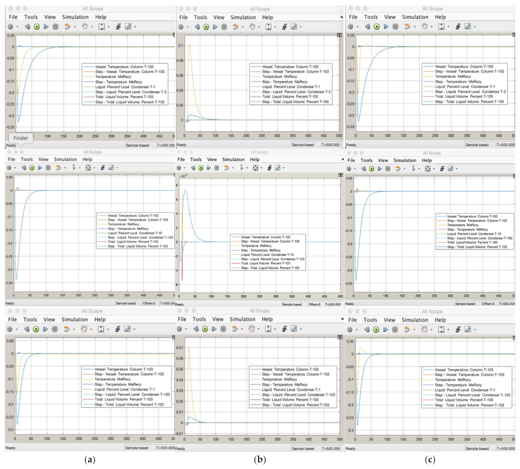
Below is the performance test results of disturbance rejection held in Simulink. Figure 5 displays the stability for all controllers. As shown on the left, the manual interference of temperature is added by increasing its original state from 81.74 °C to 85.827 °C. All controlled variables demonstrate final stability at 0. The condenser temperature (CV1) decreases when the feed-in temperature increases. It is suspected that this is caused by a slower form of top product that may result in an increase in the product temperature as well (CV2). The fine-tuned proportional-integral controller reveals a faster stabilized graphic and smaller disturbance peak than the BLT ones, but they are similar to WG. For BLT, the CV1 temperature disturbance peak reaches almost −0.32 and −0.2 for CV2, meaning the condenser temperature once reaches 58.49 °C and the MeRecy temperature decreases to 40.55 °C. They stabilize at times 150 and 50 with values back to 58.81 °C and 40.75%. In the fine-tuned controller, the CV1 peak only reaches −0.35, and CV2 and CV4 barely leave 0. All stabilize before time 100.
However, when compared with MMPC, CV1 stabilizes at a 58.167 °C condenser temperature, a 42.057 °C methanol final temperature, a 49.854% condenser level, and a 14.629% T-103 liquid volume at Stage 30. Error analysis will be further discussed in the next section.
In the middle row, the feed flow disturbance is increased from the initial value of 659.8 gmol/s to 692.72 gmol/s. Here, the fine-tuned proportional-integral controller shows the lowest oscillation. As a response towards feed molar flow increases, liquid volume in the bottom stage decreases due to a more fluid increase in heat, causing slower stage movement. The condenser temperature increases because less mixture is condensed, affecting the heat exchange process and resulting in a higher product temperature.
For MMPC results using the unisim software, the increment of CV1 stays at 59.137 °C. The BL Tune increases until 58.875 °C and fine-tunes to 58.817 °C. However, both stabilize back to 58.81 °C. The MMPC final values of CV2, CV3, and CV4 are 43.023 °C, 49.916%, and 9.9%, meaning their differences are 2.27 °C, 0.0014%, and −2.13%.
When both disturbances are added, the response is similar to when the interference is only the temperature. The condenser temperature (CV1) decreases, and the level (CV4) is barely disturbed. The MeRecy temperature increases until 0.05 °C for the BLT but barely 0.01 °C for the fine-tuning. WG has a higher oscillation than both, which shows that feed temperature interference has a higher impact, and the best controller needs to be provided. Both fine-tuned and WG PI controllers reveal a faster stabilized graphic and a smaller disturbance peak.
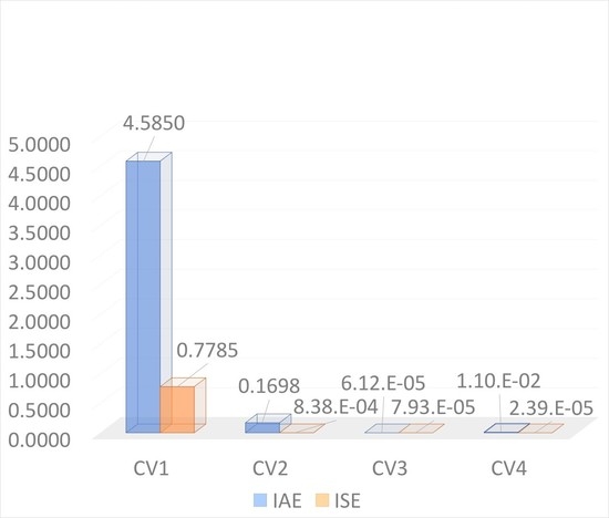
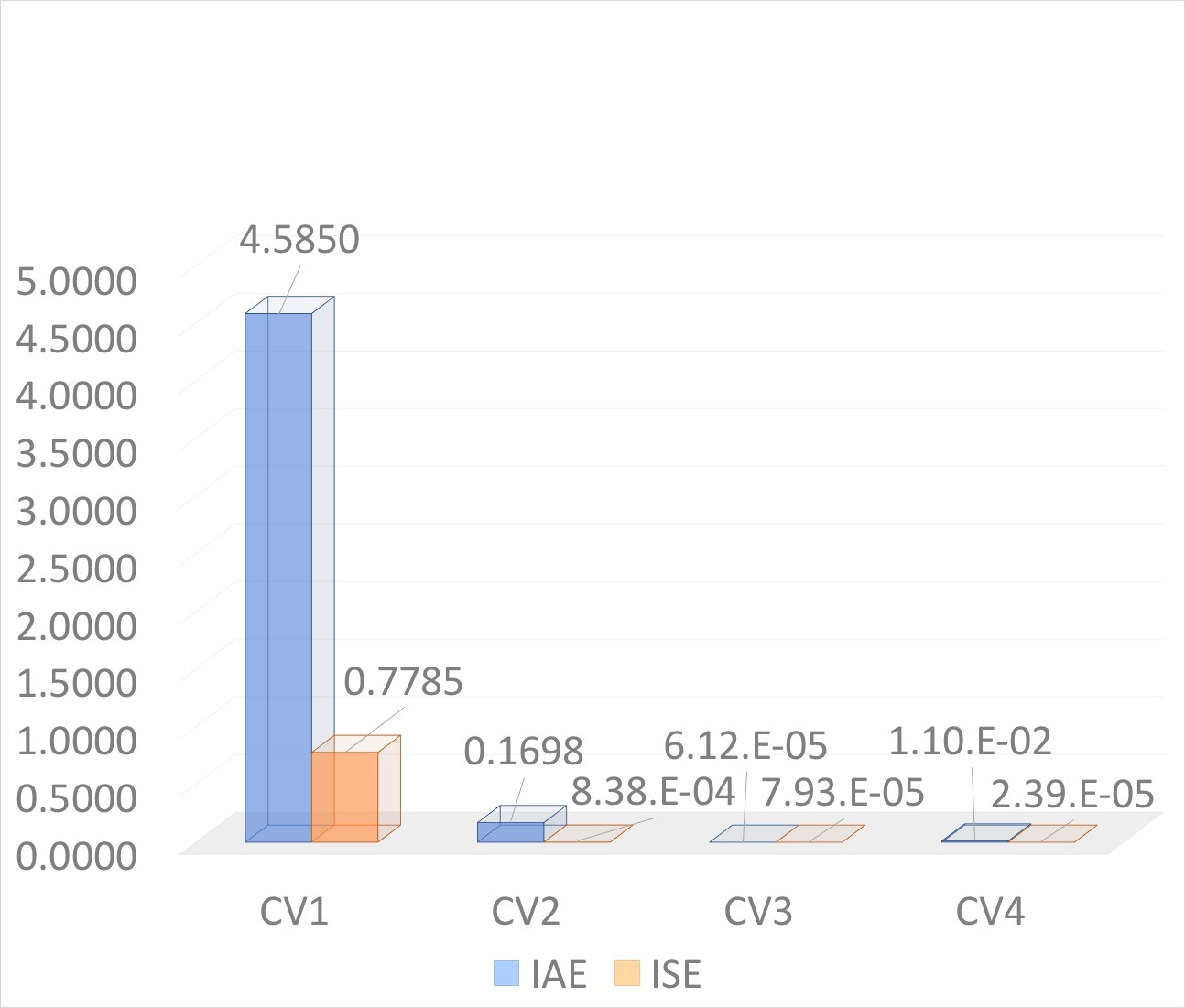
Their IAEs and ISEs are given in Table 10 and Table 11. The lowest error parameter values against temperature and flow disturbance are attributed to WG for CV1 and CV4, FT for CV2, and BLT for CV3. When both disturbances are added, the lowest error parameter values are attributed to fine-tuning for CV2. For CV1 and CV4, the parameters of Wahid and Gunawan (2015) have the lowest error values. Again, BLT has the lowest error values for CV3.
Other than during the setpoint change against itself, the liquid percent level of Condenser T-103 (CV3) controller is the best displayed by the big log-modulus tuned PI controller. For the total liquid volume percent of T-103 (CV4), the best controller is shown by that of Wahid and Gunawan (2015), except against the change of CV3.
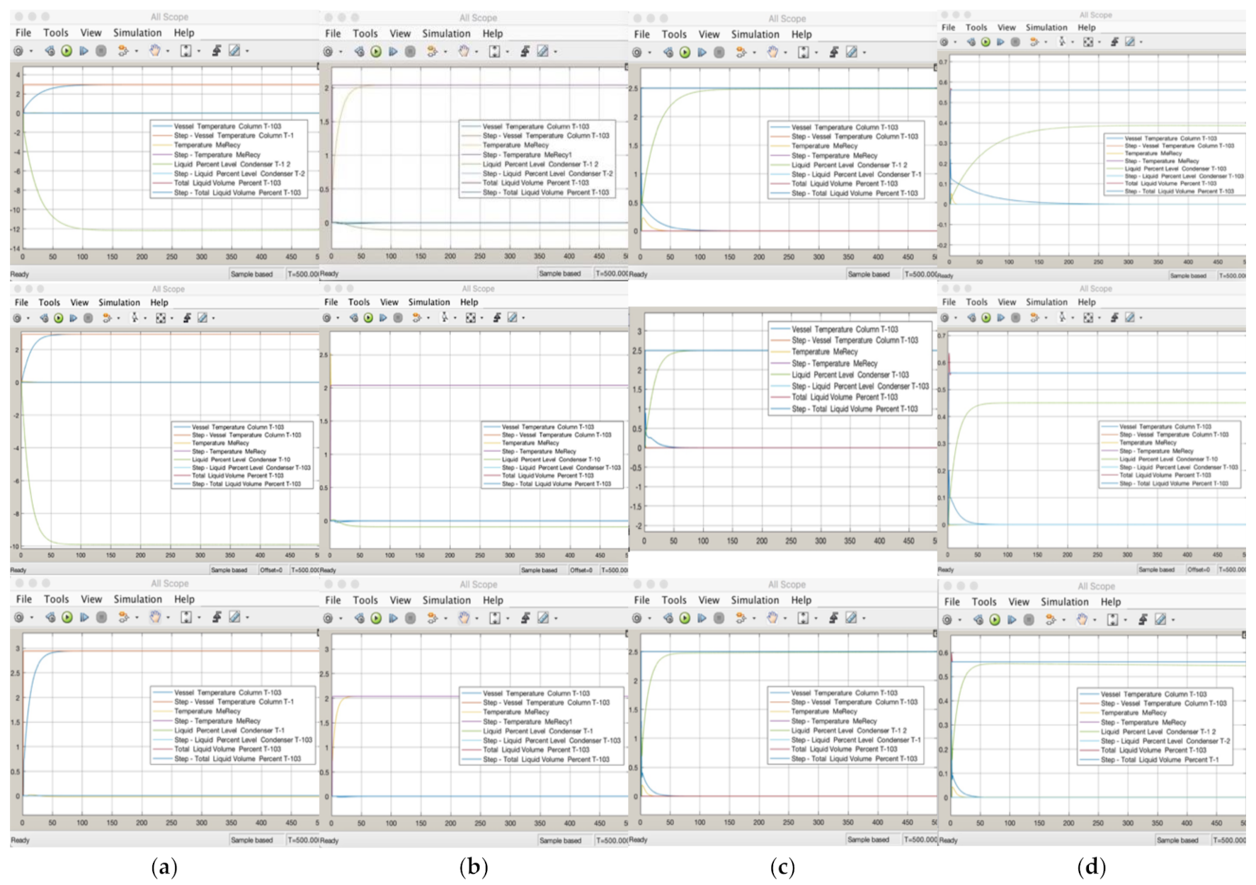
The response against setpoint changes is shown in Figure 6 and Table 12, Table 13 and Table 14. In Figure 6a, CV1 or the Vessel Condenser of the T-103 temperature is increased by 5%, from 58.81 °C to 61.7505 °C. All tuned controllers of CV1 display stability at the given final value after time 50. CV2 and CV4 are stable at 0, meaning no changes. CV3 has a decline, meaning that the value of liquid percent in the T-103 condenser decreases if CV1 is increased. If the condenser temperature changes, the column level is not affected because it is a previous process. Here, the liquid percent of the condenser decreases by about 12% by BLT tuning and almost 10% by fine-tuning. Neither affect the final temperature of the purified methanol stream. CV2 remains stable at 40.75 °C.
When CV2 is tempered, there should not be any changes towards CV1 if CV2 changes because there are no directly affected connections. Thus, in Figure 6b above, when E-101 cooler temperature changes, the rest of the controlled variables remains at approximately 0, both the condenser temperature and the column level, except for CV3.
In Figure 6c, when the CV3 setpoint is increased, CV1 and CV2 spike at the beginning of time when CV3 changes. The T-103 condenser temperature must be impacted by the change of its liquid level and thus the top product temperature. The fine-tuned PI controller has a faster response than BLT.
For CV4 setpoint tracking, the condenser temperature will be affected, and so will the output product of the purified methanol’s temperature. An increase in level means more product in the condenser, causing CV3 to increase as the CV4 setpoint is changed, indicating that G34 has a strong interaction. This is proven from the result of RGA analysis.
Wahid and Gunawan (2015) displayed the smallest and shortest deviation period for the CV1 temperature controller as well. CV2’s best improvement is shown by the fine-tuned Multi-loop PI controller. Table 15 below lists the final result parameters of this research.
To corroborate this performance, the final multi-loop PI controller parameter performance was tested in Unisim. The parameter was taken back to the simulation software and input into a PI controller tool that was later attached to the process. Although the error parameters for some are not similar or even close to similar, the PI still showed improvement compared to the MMPC performance, as shown in the Table 16 below. This shows that the accountability of a process model and a disturbance model enhances the response performance of the used controller.
The control performance of the multiloop PI is better than MMPC because MMPC is for non-linear processes modeled with Unisim, whereas, in this study, the controlled process is linear.
4. Conclusions
Based on the RGA, the correct installation of CV and MV are CV1-MV1, CV2-MV2, CV3-MV3, and CV4-MV4. To control the temperature is to control the heat flow, and to control the level is to control the flow. Proportional and Integral parameter values best to control CV1-MV1 pairing are 0.6667 and 0.3333, for CV2-MV2 are 4.9052 and 42.409, for CV3-MV3 are 0.0071 and 2.1603, also 13.5036 and 2.3776 for CV4-MV4.
Creating a disturbance model on the feed temperature and feed flow and focusing on each variable improved the controller performance in the methanol separation process in the DME Purification Plant by almost 100%; for CV1, CV2, CV3, and CV4, respectively, the IAE values are 79.49%, 99.90%, 100%, and 99.99, and the ISE values are 97.1%, 100%, 99.99%, and 100%. The linear model using FOPDT was proven reliable and realistic. Thus, in this study, multi-loop PI controllers have been proven effective against disturbance rejection, with big log modulus tuning, and the most suitable pairing. However, it is still unstable against setpoint changes. In addition to this drawback, this multi-loop PI controller has only been proven theoretically. A further implementation method on the physical hardware of a programmable logic controller (PLC) system needs to be explored.
Author Contributions
Conceptualization, A.W.; methodology, M.R.; validation, A.W.; formal analysis, M.R.; resources, A.W.; data curation, M.R.; writing—original draft preparation, M.R.; writing—review and editing, M.R.; visualization, M.R.; supervision, A.W.; project administration, M.R.; funding acquisition, A.W. All authors have read and agreed to the published version of the manuscript.
Funding
This research received no external funding.
Institutional Review Board Statement
Not applicable. The study did not involve humans or animals.
Informed Consent Statement
Not applicable. The study did not involve humans or animals.
Data Availability Statement
Publicly available datasets were analyzed in this study. This data can be found here: https://drive.google.com/drive/folders/18Dwsix0dJ4HAKXDzeqTJMn0WZWGGY7ye?usp=sharing, accessed on 9 October 2021.
Conflicts of Interest
The authors declare no conflict of interest.
References
- Ministry of Energy and Mineral Resources Republic of Indonesia. Handbook of Energy & Economic Statistics of Indonesia; Head of Center for Data and Information Technology on Energy and Mineral Resources: Jakarta, Indonesia, 2018.
- Musalaiah, M.; Engineer, T.C.; Peddintaiah, K. A Theoretical Study on Dimethyl Ether: An Alternative Fuel for Future Generations. Int. Res. J. Eng. Technol. (IRJET) 2016, 3, 238–243. [Google Scholar]
- Takeishi, K. Dimethyl ether (DME): A clean fuel/energy for the 21st century and the low carbon society. Int. J. Energy Environ. 2016, 10, 238–242. [Google Scholar]
- Falco, M.D. Dimethyl Ether (DME) Production; University UCBM: Rome, Italy, 2017. [Google Scholar]
- Solichin, A.; Sari, M.; Rahmiyati, W.Y. Production of DME from Syngas (for Oxygenates in Diesel Oil and Blending LPG): Plant Design Report; Department of Chemical Engineering, Faculty of Engineering, Universitas Indonesia: Depok, Indonesia, 2011. [Google Scholar]
- Atef, G.; Almadani, A.; Noaman, S. Manufacturing of DME from Methanol; King Fahd University of Petroleum & Minerals: Dhahran, Saudi Arabia, 2015. [Google Scholar] [CrossRef]
- Dieterich, V.; Buttler, A.; Hanel, A.; Spliethoff, H.; Fendt, S. Power-to-liquid via synthesis of methanol, DME or Fischer–Tropsch-fuels: A review. R. Soc. Chem. 2020, 13, 3207–3252. [Google Scholar] [CrossRef]
- Khaleel, A. Methanol Dehydration to Dimethyl Ether over Highly Porous Xerogel Alumina Catalyst: Flow Rate Effect. Fuel Process Technol. 2010, 91, 1505–1509. [Google Scholar] [CrossRef]
- Dyrda, K.M.; Wilke, V.; Haas-Santo, K.; Dittmeyer, R. Experimental Investigation of the Gas/Liquid Phase Separation Using a Membrane-Based Micro Contactor. ChemEngineering 2018, 2, 55. [Google Scholar] [CrossRef] [Green Version]
- Liptak, B. Instrument Engineer’s Handbook: Process Control; CRC Taylor & Francis: Boca Raton, FL, USA, 2012. [Google Scholar] [CrossRef]
- Marlin, T. Process Control: Designing Processes and Control System for Dynamic Performance, 2nd ed.; McGraw Hill: Singapore, 2015; ISBN 9780070393622. [Google Scholar]
- Wahid, A.; Gunawan, T.A. Pengendalian Proses Purifikasi DME dan Metanol pada Pabrik DME dari Gas Sintesis. Sinergi 2015, 19, 57–66. [Google Scholar] [CrossRef] [Green Version]
- Wahid, A.; Brillianto, Z.H. Multivariable Model Predictive Control (4 × 4) of Methanol Water Separation in Dimethyl Ether Production. AIP Conf. Proc. 2015, 2255, 030055. [Google Scholar] [CrossRef]
- Nandong, J. Decentralized Control Systems; Curtin University: Curtin, Malaysia, 2020. [Google Scholar] [CrossRef]
- Vu Truong, N.; Lee, M. Optimal Design of Multi-loop PI Controllers for Enhanced Disturbance Rejection in Multivariable Processes; School of Chemical Engineering and Technology Yeungnam University: Gyeoungbuk, Korea, 2007; Available online: http://psdc.yu.ac.kr (accessed on 22 July 2020).
- Biyanto, T.; Sordi, N.; Sehamat, N.; Zabiri, H. PID Multivariable Tuning System Using BLT Method for Distillation Column; IOP Publishing: Tokyo, Japan, 2018. [Google Scholar] [CrossRef]
- Farsi, M. Dynamic Modeling and Controllability Analysis of DME Production in an Isothermal Fixed Bed Reactor; Department of Chemical Engineering, School of Chemical and Petroleum Engineering, Shiraz University: Shiraz, Iran, 2015. [Google Scholar] [CrossRef] [Green Version]
- Huang, H.; Jeng, J.; Chiang, C.; Pan, W. A Direct Method for Multi-Loop PI/PID Controller Design; Department of Chemical Engineering, National Taiwan University: Taipei, China, 2003. [Google Scholar] [CrossRef]
- Kumar, R.; Anand, S.; Khulbey, A.; Jha, A.N. Design of Fractional Order Controller for Wood-Berry Distillation Column; Department of Instrumentation and Control Engineering, Netaji Subhas University of Technology: New Delhi, India, 2020; ISBN 9781728169163. [Google Scholar]
- Kalpana, R.; Harukumar, K.; Senthukumar, J.; Balasubramanian, G.; Gour, A. Multivariable Static Output Feedback Control of a Binary Distillation Column Using Linear Matrix Inequalities and Genetic Algorithm; School of Electrical and Electronics Engineering, Sastra University: Thanjavur, India, 2017. [Google Scholar] [CrossRef]
- Kalhoro, A.; Memon, S. Design of Multivariable PID Controllers: A Comparative Study; Department of Electronic Engineering, Mehran University: Jamshoro, Pakistan, 2021. [Google Scholar] [CrossRef]
- Alawad, N.; Muter, A. Optimal Control of Model Reduction Binary Distillation Column; Department of Computer Engineering, Faculty of Engineering, Mustansiriyah University: Baghdad, Iraq, 2021. [Google Scholar] [CrossRef]
- Ogunnaike, B.A.; Ray, W.H. Multivarianle Design Controller Design for Linear Systems Having Multiple Time Delays; Department of Chemical Engineering, University of Winconsin: Madison, WI, USA, 1979. [Google Scholar]
- Smith, C. Digital Computer Process Control; Intext: Scranton, PA, USA, 1972; ISBN 0700224017/9780700224012. [Google Scholar]
- Camacho, E.F.; Bordons, C. Model Predictive Control, 2nd ed.; Springer: London, UK, 2007; ISBN 9780857293985. [Google Scholar]
- Vazquez, F.; Morilla, F. Tuning Decentralized PID Controllers for MIMO Systems with Decouplers. In Proceedings of the 15th Triennial World Congress, Barcelona, Spain, 21–26 July 2002. [Google Scholar] [CrossRef]
- Krishna, G.H.; Kiranmayi, R.; Rathaiah, M. Control System Design for 3 × 3 Processes Based on Effective Transfer Function and Fractional Order Filter. Int. J. Eng. Adv. Technol. (IJEAT) 2019, 8, 637–642. [Google Scholar]
- Chau, P.C. Chemical Process Control: A First Course with MATLAB; University of California: San Diego, CA, USA, 2001. [Google Scholar] [CrossRef]
- Wahid, A.; Tanuwijaya, R. Pemilihan Metode Penyetelan Pengendali PI pada Pengendalian Pabrik Regasifikasi LNG Menggunakan Metode Skor. In Proceedings of the Seminar Nasional Teknik Kimia UNPAR, Bandung, Indonesia, 19 November 2015. [Google Scholar]
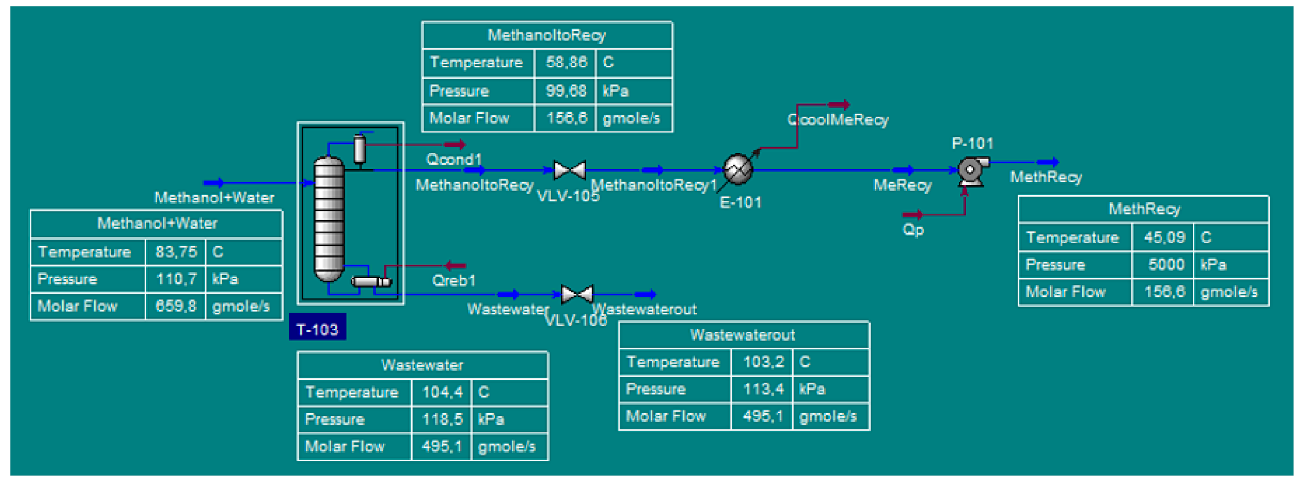
Figure 1.
Methanol purification process simulation.

Figure 2.
Process reaction curve (PRC) of (a) Method I, (b) Method II, and (c) Method III (Source: Smith, 1972; Wade, 2004).
Figure 2.
Process reaction curve (PRC) of (a) Method I, (b) Method II, and (c) Method III (Source: Smith, 1972; Wade, 2004).

Figure 3.
Block diagram of the 2 × 2 MIMO process system multi-loop controller. (Source: Nandong, 2020) [14].
Figure 3.
Block diagram of the 2 × 2 MIMO process system multi-loop controller. (Source: Nandong, 2020) [14].

Figure 4.
PRC of methanol purification controlled variables after the addition of (a) feed-in flow disturbance and (b) feed-in temperature disturbance.
Figure 4.
PRC of methanol purification controlled variables after the addition of (a) feed-in flow disturbance and (b) feed-in temperature disturbance.

Figure 5.
Responses of the methanol purification process using BLT, FT, or WG (top to bottom) with disturbance(s) of (a) feed temperature, (b) feed flow, and (c) feed temperature and feed flow (from left to right). Vessel temperature of Column T-103 (CV1) is colored blue, temperature of the MeRecy stream (CV2) is colored yellow, the liquid percent level of Condenser T-103 (CV3) is colored green, and the total volume percent of T-103 (CV4) is colored red. Step of CV1 is colored orange, Step of CV2 is colored purple, Step of CV3 is colored light blue, and Step of CV4 is colored blue. Note that the CVs are analyzed, so none are manually increasing, and thus there are no changes in the step lines.

Figure 6.
Responses against setpoint tracking using BLT, FT, and WG (top to bottom) in terms of (a) the vessel temperature of Column T-103 (CV1), (b) the temperature of the MeRecy stream (CV2), (c) the liquid percent level of Condenser T-103 (CV3), and (d) the total volume percent of T-103 (CV4). CV1 is colored blue, CV2 is colored yellow, CV3 is colored green, and CV4 is colored red. Step of CV1 is colored orange, Step of CV2 is colored purple, Step of CV3 is colored light blue, and Step of CV4 is colored blue.


Table 1.
Cooler and pump process parameters.
| Unit | Code | Objectives | Initial | Final |
|---|---|---|---|---|
| Cooler | E-101 | Cools methanol distillates | 240 ℉ | 110 ℉ |
| Pump | P-101 | To increase the recycle flow pressure | 200 kPa | 3500 kPa |
(Source: Solichin et al. 2011) [5].
Table 2.
Distillation column process parameters.
| Process Parameters | T-103 |
|---|---|
| Number of Stages | 30 |
| Condenser Pressure | 14.69 psia |
| Reboiler Pressure | 14.69 psia |
| Stream Inlet Stage | 19 |
(Source: Solichin et al. 2011) [5].
Table 3.
CV and MV of the methanol purification process.
| No | Unit Process | Controller Type | Controlled Variable | Manipulated Variable | Set Point | Actuator | Disturbance |
|---|---|---|---|---|---|---|---|
| 1 | Condenser T-103 | Temperature control | Temperature | Heat flow | 58.81 °C | Control Valve Qcond1 | Changes in the inlet feed (methanol + water) temperature and molar flow |
| 2 | Cooler E-101 | Heat flow | 40.75 °C | Control Valve QcoolMeRecy | |||
| 3 | Condenser T-103 | Level control | Column Level | Methanol to recycle Flow | 49.96% | Actuator Desired Position VLV- 105 | |
| 4 | Column T-103 | Wastewater flow | 11.22% | Actuator Desired Position VLV- 106 |
Table 4.
Relative gain array effect.
| λ | Possible Pairing |
|---|---|
| λmn < 0 | Unstable interactions |
| λmn = 1 | No interaction exists |
| λmn = 0.5 | Strong interactions |
| λmn > 1 | Interactions in the opposite direction of the variables, and stronger as value increases |
| λmn < 1 | Interactions in the same direction of the variables, and stronger as the value decreases |
Table 5.
Quick summaries of several possibilities.
| Λ | Possible Pairing |
|---|---|
| No interaction. The controller design is a SISO system. | |
| Strong interaction if 𝛿 is close to 1; weak interaction if 𝛿 << 1. |
(Source: Chau, 2001) [28].
Table 6.
Bode plot stability parameters.
| Stable | Marginally Stable | Unstable |
|---|---|---|
| Phase over frequency > gain cross over frequency | Phase over frequency = gain cross over frequency | Phase over frequency < gain cross over frequency |
| Gain margin > 1 | Gain margin = 1 | Gain margin < 1 |
| Phase margin = positive | Phase margin = 0 | Phase margin = negative |
(Source: Marlin, 2015) [11].
Table 7.
FOPDT of the methanol purification disturbance model.
| Disturbance | Variable Process | |||
|---|---|---|---|---|
| CV1 | CV2 | CV3 | CV4 | |
| Inlet Flow | ||||
| Inlet Temperature | ||||
Table 8.
Proportional integral (PI) controller parameters of the methanol purification process.
| Controlled Variable (CV) | Controller Parameter | Big Log-Modulus Tuning | Fine Tuning | Wahid and Gunawan (2015) | |
|---|---|---|---|---|---|
| 1 | Vessel Temperature of Condenser T-103 | P | 0.67 | 0.24 | 1 |
| I | 0.33 | 1.64 | 0.5 | ||
| 2 | MeRecy Temperature | P | 0.67 | 4.90 | 1 |
| I | 0.33 | 42.41 | 0.5 | ||
| 3 | Liquid Percent Level of Condenser T-103 | P | 0.01 | −67.01 | 0.01 |
| I | 2.16 | 6.75 × 10⁻¹⁹ | 1.80 | ||
| 4 | Total Liquid Volume Percent of T-103 | P | 9.00 | 3.49 | 13.50 |
| I | 1.59 | 3.56 | 2.38 | ||
Table 9.
Final value of Simulink’s step block.
| CV | Set Point | Increase 5% | Delta (Δ) |
|---|---|---|---|
| 1 | 58.81 ℃ | 61.75 ℃ | 2.94 |
| 2 | 40.75 ℃ | 42.79 ℃ | 2.04 |
| 3 | 49.96% | 52.46% | 2.5 |
| 4 | 11.22% | 11.78% | 0.56 |
| Disturbance | |||
| Feed Temperature | 81.74 °C | 85.83 °C | 4.09 |
| Feed Flow | 659.8 gmol/s | 692.72 gmol/s | 32.98 |
Table 10.
IAE comparison of MMPC and multi-loop PI against disturbance rejection.
| CV | IAE | Improvement | |||||
|---|---|---|---|---|---|---|---|
| MMPC (Wahid and Brillianto 2020) | Multi-Loop PI | Multi-Loop PI | |||||
| Big Log-Modulus Tuning | Wahid & Gunawan (2015) | Fine-Tuning | Big Log-Modulus Tuning | Wahid & Gunawan (2015) | Fine-Tuning | ||
| Feed Temperature Disturbance | |||||||
| 1 | 3.70 × 101 | 1.05 × 101 | 4.71 | 6.65 | 71.58% | 87.27% | 82.01% |
| 2 | 7.96 × 101 | 1.24 | 2.98 × 10 | 1.62 × 10⁻¹ | 98.45% | 96.26% | 99.80% |
| 3 | 6.18 | 6.26 × 10⁻⁹ | 6.84 × 10² | 7.93 × 10⁻⁵ | 100.00% | −1.10 × 10⁴% | 100.00% |
| 4 | 2.04 × 10² | 2.47 × 10⁻² | 1.10 × 10⁻² | 2.82 × 10⁻² | 99.99% | 99.99% | 99.97% |
| Feed Flow Disturbance | |||||||
| 1 | 3.75 × 101 | 3.11 × 10⁻¹ | 1.53 × 10⁻¹ | 2.09 × 10⁻¹ | 99.17% | 99.59% | 99.44% |
| 2 | 1.55 × 10² | 4.97 × 10⁻¹ | 9.20 × 10⁻¹ | 1.18 × 10⁻² | 99.68% | 99.41% | 99.99% |
| 3 | 3.32 | 1.46 × 10⁻⁶ | 1.62 × 101 | 1.87 × 10⁻⁶ | 100.00% | −385.80% | 100.00% |
| 4 | 7.41 × 101 | 1.16 × 10⁻² | 5.15 × 10⁻³ | 1.33 × 10⁻² | 99.98% | 99.99% | 99.98% |
| Feed Flow and Temperature Disturbance | |||||||
| 1 | 2.24 × 101 | 1.02 × 101 | 4.59 | 6.48 | 54.19% | 79.49% | 71.02% |
| 2 | 1.64 × 10² | 1.47 | 2.66 | 1.70 × 10⁻¹ | 99.11% | 98.38% | 99.90% |
| 3 | 1.24 × 101 | 6.12 × 10⁻⁵ | 6.69 × 10² | 7.74 × 10⁻⁵ | 100.00% | −5.31 × 10³% | 100.00% |
| 4 | 2.04 × 10² | 2.47 × 10⁻² | 1.10 × 10⁻² | 2.82 × 10⁻² | 99.98% | 99.99% | 99.98% |
Table 11.
ISE comparison of MMPC and multi-loop PI against disturbance rejection.
| CV | ISE | Improvement | |||||
|---|---|---|---|---|---|---|---|
| MMPC (Wahid and Brillianto 2020) | Multi-Loop PI | Multi-Loop PI | |||||
| Big Log-Modulus Tuning | Wahid & Gunawan (2015) | Fine-Tuning | Big Log-Modulus Tuning | Wahid & Gunawan (2015) | Fine-Tuning | ||
| Feed Temperature Disturbance | |||||||
| 1 | 2.30 × 101 | 2.03 | 8.01 × 10⁻¹ | 1.41 | 91.20% | 96.52% | 93.89% |
| 2 | 1.06 × 10² | 9.90 × 10⁻² | 1.58 × 10⁻¹ | 7.03 × 10⁻⁴ | 99.91% | 99.85% | 100.00% |
| 3 | 6.41 × 10⁻¹ | 8.31 × 10⁻⁵ | 9.53 × 10² | 1.29 × 10⁻⁴ | 99.99% | −1.49 × 10⁵% | 99.98% |
| 4 | 6.94 × 10² | 1.01 × 10⁻⁴ | 2.39 × 10⁻⁵ | 1.63 × 10⁻⁴ | 100.00% | 100.00% | 100.00% |
| Feed Flow Disturbance | |||||||
| 1 | 6.62 × 101 | 1.33 × 10⁻³ | 5.47 × 10⁻⁴ | 1.02 × 10⁻³ | 100.00% | 100.00% | 100.00% |
| 2 | 4.43 × 10² | 2.17 × 10⁻² | 4.20 × 10⁻¹ | 1.62 × 10⁻⁵ | 100.00% | 99.91% | 100.00% |
| 3 | 7.68 × 10⁻¹ | 4.66 × 10⁻⁸ | 5.41 × 10⁻¹ | 7.31 × 10⁻⁸ | 100.00% | 29.57% | 100.00% |
| 4 | 9.64 × 101 | 2.23 × 10⁻⁵ | 5.35 × 10⁻⁶ | 3.70 × 10⁻⁵ | 100.00% | 100.00% | 100.00% |
| Feed Flow and Temperature Disturbance | |||||||
| 1 | 2.68 × 101 | 1.95 | 7.79 × 10⁻¹ | 1.36 | 92.71% | 97.09% | 94.91% |
| 2 | 3.85 × 10² | 1.08 × 10⁻¹ | 1.29 × 10⁻¹ | 8.38 × 10⁻⁴ | 99.97% | 99.97% | 100.00% |
| 3 | 1.83 | 7.93 × 10⁻⁵ | 9.10 × 10² | 1.22 × 10⁻⁴ | 100.00% | −4.96 × 10⁴% | 99.99% |
| 4 | 6.94 × 10² | 1.01 × 10⁻⁴ | 2.39 × 10⁻⁵ | 1.63 × 10⁻⁴ | 100.00% | 100.00% | 100.00% |
Table 12.
IAE comparison of MMPC and multi-loop PI.
| CV | IAE | Improvement | |||||
|---|---|---|---|---|---|---|---|
| MMPC (Wahid and Brillianto 2020) | Multi-Loop PI | Multi-Loop PI | |||||
| Big Log-Modulus Tuning | Wahid & Gunawan (2015) | Fine-Tuning | Big Log-Modulus Tuning | Wahid & Gunawan (2015) | Fine-Tuning | ||
| CV1 Setpoint Change | |||||||
| 1 | 1.81 × 10² | 6.61 × 101 | 2.96 × 101 | 4.17 × 101 | 63.51% | 83.66% | 77.02% |
| 2 | 4.28 | 8.97 | 9.26 | 1.04 | −109.63% | −116.24% | 75.70% |
| 3 | 4.36 | 4.08 × 10³ | 4.16 × 10³ | 4.82 × 10³ | −93,386.24% | −9.53 × 10⁴% | −1.10 × 10⁵% |
| 4 | 2.00 × 10⁻² | 2.29 × 10⁻³ | 1.37 × 10⁻³ | 1.65 × 10⁻² | 88.54% | 93.16% | 17.70% |
| CV2 Setpoint Change | |||||||
| 1 | 4.10 × 10⁻¹ | 7.34 × 10⁻¹ | 3.28 × 10⁻¹ | 4.60 × 10⁻¹ | −79.02% | 19.95% | −12.15% |
| 2 | 5.64 × 101 | 1.83 × 101 | 8.20 | 2.71 × 10⁻¹ | 67.48% | 85.46% | 99.52% |
| 3 | 3.20 × 10⁻¹ | 3.59 × 101 | 3.73 × 101 | 4.35 × 101 | −11,112.50% | −11,546.88% | −13,493.75% |
| 4 | 2.00 × 10⁻² | 1.68 × 10⁻⁴ | 8.12 × 10⁻⁵ | 6.45 × 10⁻⁴ | 99.16% | 99.59% | 96.78% |
Table 13.
IAE comparison of MMPC and multi-loop PI (Cont’d).
| CV | IAE | Improvement | |||||
|---|---|---|---|---|---|---|---|
| MMPC (Wahid and Brillianto 2020) | Multi-Loop PI | Multi-Loop PI | |||||
| Big Log-Modulus Tuning | Wahid & Gunawan (2015) | Fine-Tuning | Big Log-Modulus Tuning | Wahid & Gunawan (2015) | Fine-Tuning | ||
| CV3 Setpoint Change | |||||||
| 1 | 7.32 | 7.51 | 5.80 | 6.97 | −2.60% | 20.71% | 4.77% |
| 2 | 4.67 | 9.21 × 10⁻¹ | 2.20 | 3.80 × 10⁻¹ | 80.29% | 52.89% | 91.86% |
| 3 | 5.59 × 101 | 4.16 × 10² | 3.92 × 10² | 1.34 × 10³ | −643.43% | −601.59% | −2301.22% |
| 4 | 5.00 × 10⁻² | 1.43 × 10⁻¹ | 4.61 × 10⁻¹ | 1.27 | −185.20% | −821.40% | −2430.00% |
| CV4 Setpoint Change | |||||||
| 1 | 5.20 × 10⁻¹ | 7.19 | 1.31 | 1.84 | −1282.31% | −151.15% | −254.42% |
| 2 | 5.30 × 10⁻¹ | 2.98 × 10⁻¹ | 7.42 × 10⁻¹ | 4.31 × 10⁻² | 43.70% | −39.91% | 91.87% |
| 3 | 5.79 | 1.73 × 10² | 1.89 × 10² | 2.19 × 10² | −2886.18% | −3.17 × 10³% | −3.68 × 10³% |
| 4 | 5.74 × 101 | 1.42 × 10⁻¹ | 1.03 × 10⁻¹ | 2.84 × 10⁻¹ | 99.75% | 99.82% | 99.51% |
Table 14.
ISE comparison of MMPC and multi-loop PI.
| CV | ISE | Improvement | |||||
|---|---|---|---|---|---|---|---|
| MMPC (Wahid and Brillianto 2020) | Multi-Loop PI | Multi-Loop PI | |||||
| Big Log-Modulus Tuning | Wahid & Gunawan (2015) | Fine-Tuning | Big Log-Modulus Tuning | Wahid & Gunawan (2015) | Fine-Tuning | ||
| CV1 Setpoint Change | |||||||
| 1 | 4.35 × 10² | 8.90 × 101 | 3.92 × 101 | 6.42 × 101 | 79.54% | 90.99% | 85.23% |
| 2 | 4.00 × 10⁻² | 1.72 × 10⁻¹ | 1.77 × 10⁻¹ | 3.37 × 10⁻² | −328.75% | −343.50% | 15.80% |
| 3 | 6.00 × 10⁻² | 3.39 × 10⁴ | 3.49 × 10⁴ | 4.71 × 10⁴ | −5.65 × 10⁷% | −5.82 × 10⁷% | −7.84 × 10⁷% |
| 4 | 5.36 × 10⁻⁷ | 9.18 × 10⁻⁸ | 4.40 × 10⁻⁸ | 9.48 × 10⁻⁶ | 82.88% | 91.79% | −1669.03% |
| CV2 Setpoint Change | |||||||
| 1 | 5.00 × 10⁻⁴ | 7.45 × 10⁻³ | 3.07 × 10⁻³ | 6.63 × 10⁻³ | −1389.60% | −514.60% | −1226.20% |
| 2 | 7.11 × 101 | 1.44 × 101 | 5.94 | 2.49 × 10⁻¹ | 79.68% | 91.6425% | 99.65% |
| 3 | 2.00 × 10⁻⁴ | 2.73 | 2.88 | 3.91 | −1.37 × 10⁶% | −1.44 × 10⁶% | −1.95 × 10⁶% |
| 4 | 8.30 × 10⁻⁷ | 4.43 × 10⁻⁹ | 3.29 × 10⁻⁹ | 2.17 × 10⁻⁷ | 99.47% | 99.60% | 73.86% |
| CV3 Setpoint Change | |||||||
| 1 | 1.00 × 10⁻² | 4.86 × 10⁻¹ | 1.85 | 1.90 | −4759% | −18,370.00% | −18,930.00% |
| 2 | 6.00 × 10⁻² | 7.18 × 10⁻³ | 1.70 × 10⁻¹ | 7.38 × 10⁻² | 88.04% | −182.83% | −23.00% |
| 3 | 3.10 × 101 | 3.71 × 10² | 3.19 × 10² | 1.22 × 10³ | −1099.23% | −930.68% | −3845.75% |
| 4 | 5.80 × 10⁻⁶ | 4.27 × 10⁻² | 5.69 × 10⁻¹ | 1.59 | −7.36 × 10⁵% | −9.82 × 10⁶% | −2.73 × 10⁷% |
| CV4 Setpoint Change | |||||||
| 1 | 4.00 × 10⁻⁴ | 4.79 × 10⁻¹ | 9.19 × 10⁻² | 1.35 × 10⁻¹ | −1.20 × 10⁵% | −2.29 × 10⁴% | −3.37 × 10⁴% |
| 2 | 5.00 × 10⁻⁴ | 6.56 × 10⁻³ | 9.32 × 10⁻³ | 6.75 × 10⁻⁵ | −1.21 × 10³% | −1764.80% | 86.51% |
| 3 | 1.30 × 10⁻¹ | 6.29 × 101 | 7.23 × 101 | 9.73 × 101 | −48,30% | −5.55 × 10⁴% | −7.47 × 10⁴% |
| 4 | 2.50 × 101 | 4.20 × 10⁻² | 2.80 × 10⁻² | 7.99 × 10⁻² | 99.83% | 99.89% | 99.68% |
Table 15.
Final controller parameter values.
| Controlled Variable (CV) | Tuning Method | P | I | |
|---|---|---|---|---|
| 1 | Vessel Temperature of Condenser T-103 | WG | 0.67 | 0.33 |
| 2 | MeRecy Temperature | FT | 4.90 | 42.41 |
| 3 | Liquid Percent Level of Condenser T-103 | BLT | 0.01 | 2.16 |
| 4 | Total Liquid Volume Percent of T-103 | WG | 13.50 | 2.38 |
Table 16.
IAE comparison of multi-loop PI in Simulink and Unisim.
| CV | IAE | Improvement | ISE | Improvement | |||||||
|---|---|---|---|---|---|---|---|---|---|---|---|
| MMPC (Wahid & Brillianto 2020) | Multi-Loop | MMPC (Wahid & Brillianto 2020) | Multi-Loop | ||||||||
| Tuning Method | Simulink | Unisim | Simulink | Unisim | Simulink | Unisim | Simulink | Unisim | |||
| CV1 Setpoint Change | |||||||||||
| 1 | 1.81 × 10² | WG | 2.96 × 101 | 2.08 × 10⁻³ | 83.66% | 100.00% | 4.35 × 10² | 3.92 × 101 | 2.65 × 10⁻⁴ | 90.99% | 100.00% |
| 2 | 4.28 | FT | 1.04 | 1.15 × 10⁻² | 75.70% | 99.73% | 4.00 × 10⁻² | 3.37 × 10⁻² | 1.92 × 10⁻⁴ | 15.80% | 99.52% |
| 3 | 4.36 | BLT | 4.08 × 10³ | 1.34 × 10⁻² | −93,386.24% | 99.69% | 6.00 × 10⁻² | 3.39 × 10⁴ | 1.83 × 10⁻⁴ | −5.65 × 10⁷% | 99.69% |
| 4 | 2.00 × 10⁻² | WG | 1.37 × 10⁻³ | 1.37 × 10⁻³ | 93.16% | 93.16% | 5.36 × 10⁻⁷ | 4.40 × 10⁻⁸ | 2.89 × 10⁻⁷ | 91.79% | 46.18% |
| CV2 Setpoint Change | |||||||||||
| 1 | 4.10 × 10⁻¹ | WG | 3.28 × 10⁻¹ | 1.27 × 10⁻² | 19.95% | 96.91% | 5.00 × 10⁻⁴ | 3.07 × 10⁻³ | 2.45 × 10⁻⁴ | −514.60% | 51.05% |
| 2 | 5.64 × 101 | FT | 2.71 × 10⁻¹ | 2.76 × 10⁻¹ | 99.52% | 99.51% | 7.11 × 101 | 2.49 × 10⁻¹ | 6.43 × 10⁻¹ | 99.65% | 99.10% |
| 3 | 3.20 × 10⁻¹ | BLT | 3.59 × 101 | 3.25 × 10⁻³ | −11,112.50% | 98.99% | 2.00 × 10⁻⁴ | 2.73 | 1.48 × 10⁻⁵ | −1.37 × 10⁶% | 92.59% |
| 4 | 2.00 × 10⁻² | WG | 8.12 × 10⁻⁵ | 1.36 × 10⁻³ | 99.59% | 93.22% | 8.30 × 10⁻⁷ | 3.29 × 10⁻⁹ | 2.78 × 10⁻⁷ | 99.60% | 66.51% |
| CV3 Setpoint Change | |||||||||||
| 1 | 7.32 | WG | 5.80 | 1.25 × 10⁻² | 20.71% | 99.83% | 1.00 × 10⁻² | 1.85 | 2.40 × 10⁻⁴ | −18370.00% | 97.60% |
| 2 | 4.67 | FT | 3.80 × 10⁻¹ | 1.11 × 10⁻² | 91.86% | 99.76% | 6.00 × 10⁻² | 7.38 × 10⁻² | 1.83 × 10⁻⁴ | −23.00% | 99.70% |
| 3 | 5.59 × 101 | BLT | 4.16 × 10² | 2.66 × 10⁻³ | −643.43% | 100.00% | 3.10 × 101 | 3.71 × 10² | 1.47 × 10⁻⁵ | −1099.23% | 100.00% |
| 4 | 5.00 × 10⁻² | WG | 4.61 × 10⁻¹ | 8.26 × 10⁻⁴ | −821.40% | 98.35% | 5.80 × 10⁻⁶ | 5.69 × 10⁻¹ | 1.10 × 10⁻⁶ | −9.82 × 10⁶% | 81.06% |
| CV4 Setpoint Change | |||||||||||
| 1 | 5.20 × 10⁻¹ | WG | 1.31 | 1.28 × 10⁻² | −151.15% | 97.53% | 4.00 × 10⁻⁴ | 9.19 × 10⁻² | 2.51 × 10⁻⁴ | −2.29 × 10⁴% | 37.25% |
| 2 | 5.30 × 10⁻¹ | FT | 4.31 × 10⁻² | 1.14 × 10⁻² | 91.87% | 97.84% | 5.00 × 10⁻⁴ | 6.75 × 10⁻⁵ | 1.91 × 10⁻⁴ | 86.51% | 61.80% |
| 3 | 5.79 | BLT | 1.73 × 10² | 3.26 × 10⁻³ | −2886.18% | 99.94% | 1.30 × 10⁻¹ | 6.29 × 101 | 1.50 × 10⁻⁵ | −4.83 × 10⁴% | 99.99% |
| 4 | 5.74 × 101 | WG | 1.03 × 10⁻¹ | 4.04 × 10⁻⁴ | 99.82% | 100.00% | 2.50 × 101 | 2.80 × 10⁻² | 2.83 × 10⁻⁷ | 99.89% | 100.00% |
| Feed Temperature Disturbance | |||||||||||
| 1 | 3.70 × 101 | WG | 4.71 | 1.61 × 10⁻¹ | 87.27% | 99.56% | 2.30 × 101 | 8.01 × 10⁻¹ | 2.78 × 10⁻² | 96.52% | 99.88% |
| 2 | 7.96 × 101 | FT | 1.62 × 10⁻¹ | 1.07 × 10⁻² | 99.80% | 99.99% | 1.06 × 10² | 7.03 × 10⁻⁴ | 1.14 × 10⁻⁴ | 100.00% | 100.00% |
| 3 | 6.18 | BLT | 6.26 × 10⁻⁹ | 9.44 × 10⁻³ | 100.00% | 99.85% | 6.41 × 10⁻¹ | 8.31 × 10⁻⁵ | 9.06 × 10⁻⁵ | 99.99% | 99.99% |
| 4 | 2.04 × 10² | WG | 1.10 × 10⁻² | 2.52 × 10⁻³ | 99.99% | 100.00% | 6.94 × 10² | 2.39 × 10⁻⁵ | 1.17 × 10⁻⁵ | 100.00% | 100.00% |
| Feed Flow Disturbance | |||||||||||
| 1 | 3.75 × 101 | WG | 1.53 × 10⁻¹ | 1.67 × 10⁻¹ | 99.59% | 99.56% | 6.62 × 101 | 5.47 × 10⁻⁴ | 4.22 × 10⁻⁵ | 100.00% | 100.00% |
| 2 | 1.55 × 10² | FT | 1.18 × 10⁻² | 1.38 × 10⁻² | 99.99% | 99.99% | 4.43 × 10² | 1.62 × 10⁻⁵ | 1.15 × 10⁻⁴ | 100.00% | 100.00% |
| 3 | 3.32 | BLT | 1.46 × 10⁻⁶ | 7.36 × 10⁻⁴ | 100.00% | 99.98% | 7.68 × 10⁻¹ | 4.66 × 10⁻⁸ | 6.73 × 10⁻⁷ | 100.00% | 100.00% |
| 4 | 7.41 × 101 | WG | 5.15 × 10⁻³ | 9.42 × 10⁻³ | 99.99% | 99.99% | 9.64 × 101 | 5.35 × 10⁻⁶ | 9.45 × 10⁻⁵ | 100.00% | 100.00% |
| Feed Flow and Temperature Disturbance | |||||||||||
| 1 | 2.24 × 101 | WG | 4.59 | 1.70 × 10⁻¹ | 79.49% | 99.24% | 2.68 × 101 | 7.79 × 10⁻¹ | 3.01 × 10⁻² | 97.09% | 99.89% |
| 2 | 1.64 × 10² | FT | 1.70 × 10⁻¹ | 1.14 × 10⁻² | 99.90% | 99.99% | 3.85 × 10² | 8.38 × 10⁻⁴ | 1.14 × 10⁻⁴ | 100.00% | 100.00% |
| 3 | 1.24 × 101 | BLT | 6.12 × 10⁻⁵ | 3.42 × 10⁻³ | 100.00% | 99.97% | 1.83 | 7.93 × 10⁻⁵ | 2.96 × 10⁻⁵ | 100.00% | 100.00% |
| 4 | 2.04 × 10² | WG | 1.10 × 10⁻² | 3.27 × 10⁻² | 99.99% | 99.98% | 6.94 × 10² | 2.39 × 10⁻⁵ | 1.43 × 10⁻³ | 100.00% | 100.00% |
Publisher’s Note: MDPI stays neutral with regard to jurisdictional claims in published maps and institutional affiliations. |
© 2021 by the authors. Licensee MDPI, Basel, Switzerland. This article is an open access article distributed under the terms and conditions of the Creative Commons Attribution (CC BY) license (https://creativecommons.org/licenses/by/4.0/).
Share and Cite
MDPI and ACS Style
Wahid, A.; Rikimata, M. Methanol–Water Purification Control Using Multi-Loop PI Controllers Based on Linear Set Point and Disturbance Models. ChemEngineering 2021, 5, 70. https://doi.org/10.3390/chemengineering5040070
AMA Style
Wahid A, Rikimata M. Methanol–Water Purification Control Using Multi-Loop PI Controllers Based on Linear Set Point and Disturbance Models. ChemEngineering. 2021; 5(4):70. https://doi.org/10.3390/chemengineering5040070
Chicago/Turabian StyleWahid, Abdul, and Monica Rikimata. 2021. "Methanol–Water Purification Control Using Multi-Loop PI Controllers Based on Linear Set Point and Disturbance Models" ChemEngineering 5, no. 4: 70. https://doi.org/10.3390/chemengineering5040070