Volume of Fluid Computations of Gas Entrainment and Void Fraction for Plunging Liquid Jets to Aerate Wastewater

Abstract

Among various mechanisms for enhancing the interfacial area between gases and liquids, a vertical liquid jet striking a still liquid is considered an effective method. This method has vast industrial and environmental applications, where a significant application of this method is to aerate industrial effluents and wastewater treatment. Despite the huge interest and experimental and numerical efforts made by the academic and scientific community in this topic, there is still a need of further study to realize improved theoretical and computational schemes to narrow the gap between the measured and the computed entrained air. The present study is a numerical attempt to highlight the air being entrained by water jet when it intrudes into a still water surface in a tank by the application of a Volume of Fluid (VOF) scheme. The VOF scheme, along with a piecewise linear interface construction (PLIC) algorithm, is useful to follow the interface of the air and water bubbly plume and thus can provide an estimate of the volume fraction for the gas and the liquid. Dimensionless scaling derived from the Fronde number and Reynolds number along with geometric similarities due to the liquid jet’s length and nozzle diameter have been incorporated to validate the experimental data on air entrainment, penetration and void fraction. The VOF simulations for void fraction and air-water mixing and air jet’s penetration into the water were found more comparable to the measured values than those obtained using empirical and Euler-Euler methods. Although, small overestimates of air entrainment rate compared to the experiments have been found, however, VOF was found effective in reducing the gap between measurements and simulations.

1. Introduction

The significance of the liquid plunging jet’s entrainment of a gas lies in achieving a large interfacial area between gas and liquid, which is useful for a large number of environmental and industrial applications. Fuel consumption optimization of ships is compromised due to the formation of a wake on the water surface associated to air being entrained across the boundary layer [1,2]. Pressurized water reactors (PWRs) face partially filled cold legs associated to emergency core cooling as a result of gas entrainment when the coolant strikes the water’s surface [3,4]. Plunging jets have been proved efficient methods to aerate industrial effluents [5,6,7,8]. Other applications include mineral-processing flotation cells [9,10] and oxygenation of cell bioreactors [11]. In another industrial process involving the casting of polymers and glass [12], promoting enhanced interaction between gas and liquid aeration is significant for the efficient formation of products.

Among the several applications of the plunging jet mentioned above, aeration and floatation of industrial effluents and wastewater treatment [8,13] represent a huge application of this method. For aerobic treatment processes, such as the activated sludge process, plunging jet aeration systems provide a simple and inexpensive method of supplying oxygen for wastewater treatment [13,14].

Bin [13] has comprehensively reviewed gas entrainment by plunging liquid jets. Numerous studies are reported in his review on single plunging jets which reveal that gas entrainment by a plunging liquid jet is a complex process. The main quantities that determine the functioning of a plummeting jet, including the reduced critical entrainment’s velocity, ue, and the amount of entrained gas rate, Q_g, which depends on parameters expressed as D_j, u_j, ρ_g, ρ_l, g, μ_j, μ_g, v’ σ, λ, respectively, where, D_j is the liquid jet’s diameter, u_j is the liquid jet’s velocity at the time of contact with the pool liquid, ρ_g is the gas density (i.e., air), ρ_l is the liquid’s density of the jet and the liquid in the pool, g is the acceleration constant due to gravity, μ_j is the liquid viscosity (i.e., water), μ_g is the gas viscosity (i.e., air), v’ is the geometry of the case has been approximated by refereeing to a characteristic length L.

The occurrence of air entrainment associated to the water jet impacting into a liquid pool has been found an efficient phenomenon to form larger interfacial areas between gas and liquid, for instance in environmental industries, plunging liquid jets can cause agitation when contacting the surface of a liquid pool to improve exchange between the gas and liquid [13,15,16]. For industrial effluent and water treatment, the influence due to the combined inertial as well as intense turbulence is to enhance the mass transfer of gases (i.e., nitrogen, oxygen, hydrogen sulphide, etc. and organic compounds). Air entrainment generally occurs due to two mechanisms that complement each other, one of these is the interfacial shear acting at the intermittent region between the water and the air, which shrinks the air boundary layer. However, the second phenomenon relates to the entrapment of the air in the vicinity of the plunging jet when striking a liquid pool [17]. Entrapment of air at the water surface causes a large scale cavity with the cylindrical shape at the bottom that is pinched off, thus forming a bubbly plume that moves downward below the impact surface of the water [18].

With a huge increase in computing power in the last few decades, several numerical models; two-fluid [19,20]; large eddy simulation (LES) [21,22], direct numerical simulation (DNS) [23], Euler-Euler method [22,24] and many others have been built to determine understanding of multiphase, gas and liquid plunging jets. Among these VOF, proposed by Hirt and Nichols [25], is useful to simulate the interface interaction between gas and liquid flows. Ma et al. [19] applied a Eulerian/Eulerian two-fluid computational multiphase fluid dynamics (CMFD) model along with a supplement sub-grid air entrainment model to predict the distribution of void fraction in vertical plunging water jets. Miwa et al. [4] made use of analytical and dimensionless numbers such as the Weber number and Laplace length scale to propose a predictive model for the computation of air entrainment ratio (entrained air rate/impinging jet rate), which deviated from the experimental values by about 15.9%. Yin et al. [20] used the volume of fluid and coupled level set method to investigate the numerical response of a vertical plunging jet. The computational values were in accordance with reported literature values on the subject matter. Different vertical jet parameters such as the air void fraction, liquid velocity field, and turbulent kinetic energy were analyzed by altering the length between the still water level and the nozzle exit. The velocity of the nozzle exit had no role in the size and shape of inpinging bubbles. A revised predictive equation relating the axial separation and the centerline velocity ratio was formulated with the help of data for the coupled level set and volume of fluid methods, and it exhibited a greater predictability capacity than the mixture and level set methods. A comparison was drawn between turbulent kinetic characteristics such as radial and vertical distribution and the highest value location to that of submerged jets.

Several studies have been performed to track the motion of the free surface [21,22], the distortion of the interface between liquid and gas in columns [23,24], and the VOF has been applied to visualize both the plunging of the liquid jet into the still liquid and the subsequent entrained bubble plume phenomena [25,26].

The present attempt aims to focus on air being entrained by a water jet striking a still water pool using the VOF gas-liquid model. The Navier-Stokes equations are solved using the CFD code ANSYS-Fluent. The objective of the numerical investigation is to validate the applicability and accuracy of the VOF model to replicate a circular water jet sinking into a still water pool. A VOF scheme along with PLIC proved effective to characterize the distinction between the gas and liquid phase, which can prove useful in the present case to determine the bubbly plume and void fraction along the plume. However, our main emphasis is to determine the distribution of air void fraction at various depths of the plume from the water-free surface and its corresponding impact on the values of the air entrainment rate.

2. Methodology

2.1. Physical Parameters

The schematic illustration in Figure 1 shows a vertical plunging water jet of diameter D_j, which intrudes into the still surface of a water tank at a velocity u_j. The relevant dimensionless numbers, that describe the physics of the phenomenon are the Reynolds number (Re), Froude number (Fr), and Weber number (We). Reynolds number can be expressed as:

$$Re=\frac{{\rho }_w{u}_j{D}_j}{{\mu }_w}$$

(1)

where, $u_j$ is the jet’s velocity when impacting the still surface of the water pool, D_j is the jet’s diameter at the instance when the jet impacts the still surface of the water, ${\rho }_w$ is the water density, i.e., 1000 kg/m³ and ${\mu }_w$ is the water’s viscosity, i.e., 1 × 10⁻³ pa.s. Froude number is expressed as:

$$Fr=\frac{u_j}{\sqrt{g{D}_j}}$$

(2)

where, g is the gravitational acceleration, i.e., 9.8 m²/s. Weber number is written as:

$$We=\frac{{\rho }_w{u}_j^2{D}_j}{\sigma }$$

(3)

where, $\sigma$ is the surface tension corresponding to the air-water interface, 0.072 Nm⁻¹.

2.2. Numerical Scheme

The computational simulation has been conducted utilizing the commercial code Fluent applying VOF to characterize the multiphase flow. The VOF model, developed by Hirt and Nicholas [27], can track the interface between the two phases, so it can be used in all those studies where an interface between two phases exists. A two-equation, k-ε scheme using standard wall values in the vicinity of the wall layer has been applied to describe the turbulence.

The VOF has been applied here to solve multiphase flows. The VOF method deals with flow equations through averaging them in terms of volume to attain a group of equations, whereas the interface between the gas and liquid can be followed by applying a phase marker (α), better named volume function, which can be expressed as: (i) If α = 1 (i.e., computational cell occupies phase 1, e.g., liquid), (ii) If α = 0 (computational cell occupies phase 2, e.g., gas), (iii) 0 < α < 1 (both phases are present and an interface exists within the computational cell). For those cells containing either phase 1 or 2, the formulation consists of mass conservation equations and momentum conservation equations containing properties of the phase present in the cell. If both phases exist within the cell, then the properties of the air and water mixture are evaluated through a mean voidage of the fluids present within the respective cell, thus ensuring to acquire a single set of equations by averaging the variables, for the present case, these variables are density and viscosity, their averaging is expressed as:

$$\rho =\alpha {\rho }_l+\left(1-\alpha \right){\rho }_g$$

(4)

$$\mu =\alpha {\mu }_l+\left(1-\alpha \right){\mu }_g$$

(5)

Using averaging variables and considering that across the interface, the velocity corresponding to the two phases is uniform, the continuity and momentum equations [28,29] expressed as [30,31]

$$\frac{\partial \rho }{\partial t}+\nabla .\left(\rho \mathit{u}\right)=0$$

(6a)

$$\frac{\partial }{\partial t}\rho \mathit{u}+\nabla .\left(\rho \mathit{u}\mathit{u}\right)=-\nabla p+\nabla .\left(\mu \nabla \mathit{u}\right)+\rho g+F_S$$

(6b)

where, F_S symbolizes the continuum surface force (CSF) [30,32]. This force acts across the interface, containing the interfacial and subsequent surrounding cells. F_S can be expressed as:

$$F_S=\sigma \frac{{\rho }_l}{\frac{1}{2}\left({\rho }_l+{\rho }_g\right)}\kappa \nabla \alpha$$

(7)

where $\kappa$ represents the curve of the surface due to air or water on it. $\kappa$ can be computed [31,32] as:

$$\kappa =-\nabla .\overrightarrow{\mathit{n}}=-\nabla .\frac{\nabla \alpha }{\left|\nabla \alpha \right|}$$

(8)

where, $\overrightarrow{\mathit{n}}$ is the unit vector representing the surface perpendicular to the interface, however, at the wall, the surface normal to the computational cell, adjacent to the wall will be considered [30,32,33], $\overrightarrow{\mathit{n}}$ is expressed as:

$$\overrightarrow{\mathit{n}}=\overrightarrow{{\mathit{n}}_x}cos\theta +\overrightarrow{{\mathit{n}}_y}sin\theta$$

(9)

where $\theta$ is the angle between the interface and the wall and $\overrightarrow{{\mathit{n}}_x}$ and $\overrightarrow{{\mathit{n}}_y}$ stand for the unit vectors along tangential and normal to the wall, respectively. However, this is to confirm that all simulations that have been obtained here, are at a contact angle of 90° from the wall.

Since the volume fraction, α, is a property of the fluid, which changes along with the fluid, thus, its evolution is dictated by the simple advection relation, expressed as [34]:

$$\frac{\partial \alpha }{\partial t}+\nabla .u\alpha =0$$

(10)

Due to the fact the VOF model is more flexible and efficient compared to others used to track liquid-gas interfaces, the VOF has become useful in examining a wide range of gas-liquid problems [21,35,36]. Progression of the interface as a function of time between the gas and liquid is tracked in the computational cell using scheme, piecewise linear interface construction (PLIC). As prescribed by Youngs [37], the method considers a linear form of the interface between the two phases within all those cells where the two phases meet each other. Linear behavior of the interface within a cell (Figure 2) and distributions of the normal and tangential velocity at the face have been used to compute the advection of fluid (Equation (10)) across each face of the cell. Subsequently, the void fraction in every cell (α) is determined owing to the fluxes, computed in the previous cell.

Turbulence Equations

The liquid leaving the nozzle has a velocity high enough to be in a turbulent regime. The gas entrapped due to the liquid jet interacting the surface of the still liquid pool and the gas-liquid two phase flow thus formed, plunge into the pool of liquid at a mixed velocity in the range of turbulent flow. Thus, it is reasonable to compute the gas-liquid jet flow in the liquid pool by application of equations for turbulent quantities acquired by the liquid and gas. The flow variables (e.g., velocity, pressure, etc.), contain mean and fluctuating components. Thus, incorporating the instantaneous equations (Equation (6a,b)) having decomposed variables and utilizing averaging of Reynolds stresses to the Navier-Stokes equations, along with the kinetic energy, k, of turbulence, and its dissipation rate, ε. After dropping the overbar on the mean variables for convenience, The Reynolds-averaged equation after ignoring the overbar for mean quantities can be expressed in a general form as:

$$\frac{\partial \left(\rho \phi \right)}{\partial t}+div\left(\rho \mathit{u}\phi \right)=div\left({\Gamma }_{\phi }grad\phi \right)+S_{\phi }$$

(11)

where $\phi$ represents the scalar variable, ${\Gamma }_{\phi }$ is the diffusion coefficient and $S_{\phi }$ is the source term. The representation of these quantities for different variables are given in

Table 1. Source terms and values of coefficients of Generic Transport Equations [37].

Equation	$\mathit{\phi }$	${\mathbf{\Gamma }}_{\mathit{\phi }}$	${\mathit{S}}_{\mathit{\phi }}$
Continuity	$\phi /\rho$	0	0
Radial momentum	v	μeff	$-\frac{\partial p}{\partial r}+\frac{\partial }{\partial z}\left({\mu }_{eff}\frac{\partial u}{\partial r}\right)+\frac{1}{r}\frac{\partial }{\partial r}\left({r\mu }_{eff}\frac{\partial v}{\partial r}\right)-\frac{2{\mu }_{eff}v}{r^2}$
Axial momentum	u	μeff	$-\frac{\partial p}{\partial z}+\frac{\partial }{\partial z}\left({\mu }_{eff}\frac{\partial u}{\partial z}\right)+\frac{1}{r}\frac{\partial }{\partial r}\left({r\mu }_{eff}\frac{\partial v}{\partial z}\right)+g$
k Equation	k	$\mu +\frac{{\mu }_l}{{\sigma }_k}$	${\mu }_t\left[{\left(\frac{\partial u}{\partial r}+\frac{\partial v}{\partial z}\right)}^2+2{\left(\frac{\partial u}{\partial z}\right)}^2+2{\left(\frac{\partial v}{\partial r}\right)}^2+2{\left(\frac{v}{r}\right)}^2\right]-\rho \epsilon$
ε Equation	ε	$\mu +\frac{{\mu }_l}{{\sigma }_k}$	$C_1\frac{\epsilon }{k}{\mu }_t\left[{\left(\frac{\partial u}{\partial r}+\frac{\partial v}{\partial z}\right)}^2+2{\left(\frac{\partial u}{\partial z}\right)}^2+2{\left(\frac{\partial v}{\partial r}\right)}^2+2{\left(\frac{v}{r}\right)}^2\right]-C_2\rho \frac{{\epsilon }^2}{k}$

. Also, the radial (r) and axial (z) momentum equations along with k and ε equations and values of the respective constants appearing in these equations are also part of this Table.

$${\mu }_t=C_{\mu }\rho k^2, {\mu }_{eff}=\mu +{\mu }_t, C_{\mu }=0.09, C_1=1.44, C_2=1.92, {\sigma }_k=1.0, {\sigma }_{\epsilon }=1.3$$

Transport equations relating to momentum are solved to determine turbulence quantities of the two-phase flow by sharing the variables k and ε as well as the Reynolds stresses (i.e., −ρu’u’, −ρu’v’, u’ and v’ are fluctuating velocities along with the axial and transverse flow) by the phases across the flow. However, in the governing equations for turbulent production (k) and its dissipation (ε), presented in Table 1, the consequence of turbulence (i.e., Reynolds stresses) is linked to the average flow through the standard k-ε turbulence model [38]. The standard version of the turbulence model has been chosen in our study here due to the sensible computing time and is useful for high Reynolds number flows.

2.3. Simulation Plan

Geometry, Mesh, and Boundary Conditions

The 2d meshed domain of the front section of the plunging liquid jet assembly is shown in Figure 3. The meshed domain is used to compute the liquid jet plunging into the pool of still water with subsequent gas entrainment as well as the development of the bubbly plume. The computational domain consists of a 0.15 m radius, where the height varies between 0.397, 0.42 and 0.47 m, which comprises the liquid pool’s depth (0.32 m), nozzle pipe (50 mm), and liquid jet’s length, with values of 27, 50 and 100 mm. The liquid jet’s lengths adopted here are due to the nozzle sizes, i.e., 5, 6.83, 12.5 and 25 mm, which have been chosen here to follow Chanson’s [39] experimental setup. The dimensions of the Chanson’s experimental tank are sufficiently large so as not to have any impact on the contact of the water jet in the vicinity of the water-free surface. Here, the dimensions of the domain, including sizes of the water jet and the water pool (i.e., r = 0.15 m and h = 0.47 m) are sizeable enough that the boundaries have no influence, however, the jet’s domain is much smaller than the pool dimensions. Due to the preference of 2d geometrical scheme and symmetry boundary conditions, the meshed region is reduced to about 25% of the entire geometry, which is useful to reduce the computing time as well as falling within the limitations of the computing grid storage.

The inward flowrate exiting the nozzle located at the top of the water free surface and the out rate of the geometry is located at the bottom, also, wall and outlet pressure constitute the boundary conditions [40]. Water flowing through the nozzle follows a constant mean velocity profile. At the wall, no slip has been assumed. Further, an open boundary condition is considered to model the top of the domain with gauge pressure 0 Pa. However, the outlet flow from the horizontal section of the tank should follow pressure outlet conditions.

Clustering is applied towards the centerline of the liquid jet and the top water free surface to track the phases owing to the liquid and the gas phases, along with the deformation of the interface between the gas and the liquid since the tiniest gas bubble experienced in the experiment involving plunging water jet utilizing tap water is nearly 0.7 mm [39]. Thus, the cell sizes being retained are of asize smaller than the tiniest bubbles within the plume.

The fluid domain can be divided into two regions: the region that has to inhibit the jet impingement as well as the interaction regions, appropriately referred here as region of interest (ROI) between the impinged jet and the surrounding water, the mesh size in the region of interest (ROI) may approximately be within 0.01–0.03 mm, whereas in the region that is external to the main flow region (ROI) the mesh size has been keep a little coarse which is around 0.7–0.85 mm. In this way we have tried to reduce the total number of meshes with the best-attained results for the parameters of our concern (i.e., jet impingement length and the jet diameter) with the optimized meshing.

Along the region surrounding the centerline, the cells are quadratic having excellent computational prospects owing to skewness factor and orthogonal quality [41]. At all faces of the computational cell, boundary values for physical and flow properties are specified, which include gas and liquid velocity components, acting pressure (which is atmospheric pressure in the present set-up), the level function, the gas number density, the turbulent kinetic energy, k, and the turbulent dissipation, ε. To model the liquid jet at the top surface of the domain, the vertical share of the jet’s velocity is set as the nozzle outlet velocity, whereas, all remaining components of the velocity relating to the liquid and the gas as well as the function owing to the bubble’s number density are considered as zero. As stated, before that for pressure, a zero-gradient boundary condition has been set, however, the function associated with the level set has been considered such that the periphery of the liquid’s jet coincides with the level function having the zero, whereas, its value elsewhere by application of the level function is chosen to specify its zero value that coincides with that of the periphery of the liquid jet, whereas, its value elsewhere is equivalent to the distance from the level setting as zero. The model variables due to the turbulence, k, and ε, relating to their free-stream values as 9 × 10⁻⁴/Re and 0.9, respectively [21] have been set, which, have been verified to be significantly small so as to not affect the simulations.

For computations relating to fluid volumes, the mass rate at outlet boundaries has been set as less than 10⁻⁶ and the 2-D derivatives were used in the conservation equations are discretized by the use of the quick scheme, while, geometrical re-construction has been applied to achieve discretization of the void fraction in advection Equation (10). The pressure-velocity coupling has been achieved through the algorithm, pressure-inherent with the splitting of operators, PISO [42], whereas, time discretization is used as the inherent first order function applicable to the conservation equations.

An extensive grid independence test was conducted by varying the mesh size with the same Hex type of mesh elements. The varying mesh size with the total number of meshes along with the its effect on the penetration length and jet diameter has been presented in

Table 2. Grid Independence Test.

Case No.	Jet Velocity (m/s)	Mesh Size (Millions)	Element	Type	Mesh	Provision	Jet Penetration Length/Dia
01	1.7–15.7	0.31	Hex	Cooper	Fine	More fine in upper region near the jet impingement zone up till the middle of the rig	27.3–39.7/6.83–11.2
02	1.7–15.7	0.35	Hex	Cooper	Fine	More fine in upper region near the jet impingement zone up till the middle of the rig	31.8–41.2./7.9–13.2
03	1.7–15.7	0.37	Hex	Cooper	Fine	More fine in upper region near the jet impingement zone up till the middle of the rig	34.2–45.7/10.4–17.1
04	1.7–15.7	0.41	Hex	Cooper	Fine	More fine in upper region near the jet impingement zone up till the middle of the rig	37.88–49.12/12.7–20.41
05	1.7–15.7	0.43	Hex	Cooper	Fine	More fine in upper region near the jet impingement zone up till the middle of the rig	55.79–67–56/14.77–22.18
06	1.7–15.7	0.48	Hex	Cooper	Fine	More fine in upper region near the jet impingement zone up till the middle of the rig	74.58–89.18/18.79–24.87
07	1.7–15.7	0.57	Hex	Cooper	Fine	More fine in upper region near the jet impingement zone up till the middle of the rig	84.58–99.98/19.55–24.98
08	1.7–15.7	0.64	Hex	Cooper	Fine	More fine in upper region near the jet impingement zone up till the middle of the rig	85.58–99.99/19.55–24.99
09	1.7–15.7	0.69	Hex	Cooper	Fine	More fine in upper region near the jet impingement zone up till the middle of the rig	85.58–99.99/19.55–24.99
10	1.7–15.7	0.75	Hex	Cooper	Fine	More fine in upper region near the jet impingement zone up till the middle of the rig	85.58–99.99/19.55–24.99

.

Grid independence tests show that upon varying the density of the meshes from 0.31 million to 0.75 million, the highest values of the jet penetration length to the diameter of the jet has been found to be equal to its highest values i.e., (jet penetration length/jet dia 84.58–99.98/19.55–24.98). The highest values of the jet penetration length/jet dia has been achieved at 0.57 million meshes. After that computations were obtained for higher mesh sizes, however, the values for both quantities only differed by 1.0–0.01/0–0.01. Thus in order to save computational resources and time it was decided to continue with the 0.57 million meshes with the provision that a higher mesh resolution has to be used in the area where the jet impingement occurred all the way till the end of bubbly jet. As the total number of cases ranged to 9 for each mesh density thus we presented the cumulative results of the grid independence in the form of the ranges for the properties of interest i.e., the jet penetration length and the jet dia. in Table 2.

3. Numerical Results

To achieve similarity between the computations and the experimental results, non-dimensionized equations have been set to achieve right values for the jet’s size and the jet velocity that lead to Reynold’s numbers of 12,050–105,600 and Froude numbers ranging from 5 till about 9, which correspond to the experimental liquid jet velocity (1.79 m/s–4.4 m/s) analogous to the empirical nozzle dia (6.83, 12.5 and 25 mm). These values were considered for the purpose of comparison with the simulations relating to the void fraction. For evaluation of simulated outcomes for penetration of bubbly plume, experimental values [43] related to nozzle dia (0.3, 1.3, 2.4 mm) and jet velocity, ranging from 6.79–15.7 m/s, were used to evaluate the accuracy of the simulations. All these details including the geometrical dimensions and fluids properties along with the respective values of Re and Fr are summarized in

Table 3. (a) Geometry of Plunging Liquid Jet. (b) Operating Conditions and Fluid Properties.

(a)
SIM No.	Nozzle Dia (mm)-DN			Jet Dia (mm)-DJ			Jet Length (mm)-LJ
1	25			24			100
2	12.5			12.5			50
3	6.83			6.83			27.3
4	0.3, 1.3, 2.4			0.3, 1.3, 2.4
(b)
SIM No.	Nozzle Dia (mm)-DN	Jet Dia (mm)-DJ	Jet Length (mm)–LJ	Jet Velocity (m/s)	Profile Locations (m)	Fluid Properties and Details	Frj	Rej
1	25	24	100	3.5	0.8DJ, 1.2DJ, 2DJ	Tap water, μw = 1.015 × 10−3 Pa.s	7.2	82,760
				4.1		ρw = 1000 kg.m−3	8.4	96,950
				4.4		σ = 0.055 N/m	9	104,040
2	12.5	12.5	50	2.42			7.1	29,805
				3.04			8.8	37,440
				3.46			10	42,615
3	6.83	6.83	27.3	1.79			7.1	12,050
				2.16			8.5	14,540
				2.49			9.7	16,760
4	0.3, 1.3, 2.4	0.3, 1.3, 2.4		9.83–12.0, 1.86–15.7, 2.92–6.79	Penetration Depth		181.2–221.2, 16.47–139, 19–44.3	2949–3600, 2418–20410, 7008–16296

.

Simulations have been performed initially iterating for a steady liquid phase alone. A steady-state solution has been achieved after time iterations of approximately 2000 with 0.015 dimensionless time, which is equivalent to real-time of nearly 0.1 ms. The steady conditions have been verified by inspecting no change in the time-averaged quantities by raising the number of iterations. Thus, before moving on to the simulations for the bubbly flow, a steady flow of the liquid phase alone has been set as the initial condition.

The simulation involving bubbly flow has been initiated by setting on the multiphase model. The bubbly flow simulation has been obtained with the time step the same as of the single phase, and bubbles travel vertically down across the computational domain towards the region where the bubbles’ buoyancy is sufficient to enable the bubbles to move up. However, for simulating gas entrainment and void fraction profiles along with a depth of water pool at 2D_j from the contact surface, here air entrainment and void fraction measurements have been achieved experimentally. The bubbles have taken nearly 600 time periods to cover the computational domain equivalent to 2D_j. The time-averaged void fractions have been obtained after attaining a steady value after approximately 3000 time periods. The measurements such as gas entrainment and void fraction, made by [39] involving water jet sinking into the water pool have been used for comparison with the simulations.

3.1. Gas Entrainment and Developing Bubbly Regime

Sequential illustrations of the simulations presented in Figure 4 show the formation of a gas plume within the liquid pool. VOF simulation exhibits entrainment of the air by the water jet, that has been driven deeper in the tank. The entrained gas bubbles have been advected by the downward flow to form a plume. The depth of the plume associates with the momentum of the water jet, however, bubbles can only be driven down to a depth where the bubble’s buoyancy overcomes the momentum owned by the liquid jet, thus, bubbles rise due to the buoyancy to reach the surface of the pool, where they the gas separates the liquid. Similar computational results were found by [18,21,25]. The volumetric downward gas rate at a given level below the surface is given by:

$$Q_g\left(z\right)={{\displaystyle \int }}_z^{}{q}_{g}dS$$

(12)

where q_g is the volumetric rate flux of the gas. Since the 1980s, empirical predictive modeling equations relating to plunging liquid jets have been proposed [15,44,45], however, simple relations based on geometry conditions have been proposed in these studies and absolutely no influence due to the physical properties of the fluids into the predicting modeling has been emphasized in them. Bin [13] was the first who has realized the impact of fluid properties into his empirical predictive modeling:

$$\frac{Q_g}{Q_j}=0.04F{r}^{0.28}{\left(\frac{h_p}{D_N}\right)}^{0.4}$$

(13)

where Q_g is the downward vertical gas flux density or gas (air) entrainment rate (m³/s), Q_j is the liquid volumetric rate (m³/s) and h is the depth of the plume from the impact (m). The above equation has been found agreeable with the data following conditions falling within, $\frac{L_j}{D_N}\le 100,\frac{L_j}{D_N}\ge 10 \mathrm{and} F{r}^{0.28}{\left(\frac{L_j}{D_N}\right)}^{0.4}\ge 10$. The relation has been observed to agree with an error of about ±20%, compared to experimental values for air entrainment, relating to the present geometrical setup involving air and water.

The present simulated air entrainment ($\frac{Q_g}{Q_j}$) values along with Chanson [39] experimentally measured values and Bin’s [13] correlations as well as Euler-Euler simulated values [25], are summarized in

Table 4. Air Entrainment to Water Rate Ratio.

	Dj(m)	uj (m/s)	Lj (m)	Fr	Qair/Qw
Bin [13] Correlation
	0.024	3.5	0.1	7.2	0.12
	0.005	2.54	0.01	11.47	0.104
	0.00683	2.49	0.027	9.62	0.131
Chanson’s Values [39]
	0.024	3.5	0.1	7.2	0.11
	0.00683	2.49	0.027	9.62	0.193
Euler-Euler [25]
	0.005	2.54	0.01	11.47	0.5
VOF Simulations
	0.024	3.5	0.1	7.2	0.19
	0.005	2.54	0.01	11.47	0.24
	0.00683	2.49	0.027	9.62	0.26

. The VOF simulations have revealed a closer agreement with air entrainment values determined from Bin’s correlation and experiments compared to the Euler-Euler simulations. This shows that VOF scheme is effective to trace the air-water interface.

Moreover, the gas entrainment in the present situation is modeled using the advection (Equation (10)) that provides sufficient protection from the errors in entrainment caused due to the numerical method, whereas, within the region across the developing bubbly plume, the distribution of the bubbles is not influenced by the interfacial forces as only surface tension has been included in the momentum equation. For improvement in the bubble’s distribution within the plume’s profile across the depth of the water pool, there is a need to improve the modeling by enhancing the interfacial interaction between gas and liquid.

3.2. Penetration Depth

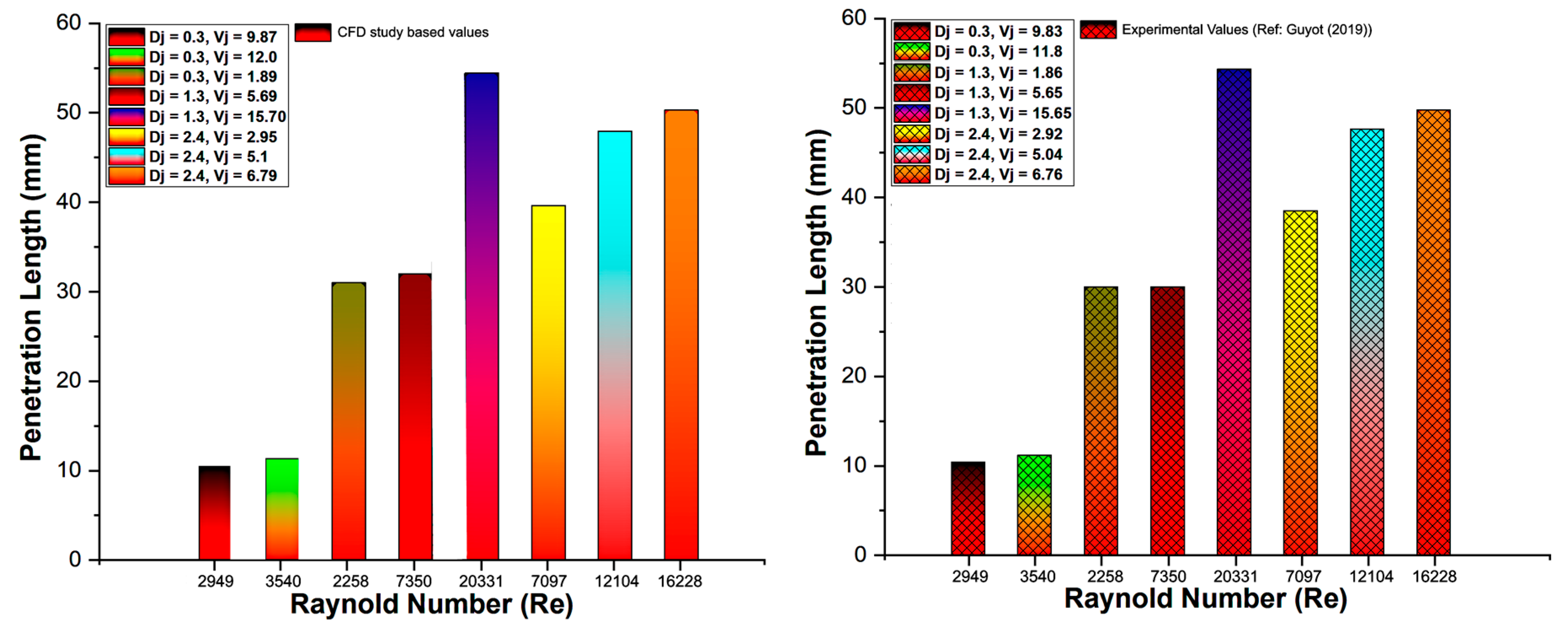
After nearly four seconds of physical time, the gas plume reaches a steady penetration depth, h_p, below the water free surface. The simulated values for the penetration of bubbly plume can be seen in Figure 5, also recent data for the circular plunging jet from Guyot [43] on the penetration of bubbly plume has been included in this figure. It’s interesting to express here the empirical correlation proposed by Bin [13] for plume’s penetration ($h_p$):

$$h_p=0.42u_j^{1.25}{D}_N{Q_g}^{-0.25}$$

(14)

The relation has been used to determine the depth of the gas plume as per the sizes of the configuration. The relation is applicable for liquid jet nozzle sizes that vary from 3.9 mm to 12 mm, whereas, and for a pool depth (h) about 0.50 m or less, with the error of ±20%. VOF simulated values for $h_p$ higher than both experimental [39] and predictive values of the above equation. This equation can also be expressed alternatively [18] as:

$$h_p=2.1u_j^{0.775}{D}_N^{0.67}$$

(15)

The relation reveals that the bubbly plume is independent of the quantity of air being entrained and it only depends on the jet’s velocity and the nozzle size.

Table 5. Bubbly Plume Penetration Depth(m) at u_j = 2.54 m/s and D_N = 5 mm.

Experimental	Bin’s Correlation	Euler-Euler	VOF Simulation
0.23	0.131	0.10	0.3

provides a summary of the penetration depth of bubbly plume below the impact surface for a jet velocity of 2.54 m/s and nozzle dia of 5 mm. The VOF computed penetration depth that follows the continuous entrainment regime against the operating condition is 0.3 m, which exceeds both the empirical correlation (Equation (14)) and the experimental values. However, with the Euler–Euler scheme, the plume depth doesn’t reach as much as the experiment (Equation (14)).

3.3. Void Fraction

The instant void fraction values have been averaged over time to obtain a steady mean void fraction over 3000 iterations, which have been averaged again along the circumference. The mean simulated values of void fraction are compared with averaged values of void fraction experimentally measured by Chanson [39], obtained under similar operating conditions as in the simulations described here. The experimental void fractions determined by Chanson [39] have been measured along a horizontal axis that passes through the jet’s center. These measurements have been averaged by including results either sides of the jet to curtail the error owing to the measurements. It is known that the flow attains the status of fully developed at 40D_J [46], which is much outside the computational domain being used here. Subsequently, the plume’s depth such as 0.8D_j, 1.2D_j, and 2D_j from the impact surface, have been chosen for simulated void fraction profiles across the bubbly plume.

It has been described under the above topics that the bubbles have been entrained through the impact between the liquid jet and the receiving pool. Further from the impact surface, the bubbles move both inside and outside radially, as the two-phase mixture travels deep into the water pool. All this can be seen in a sequence of snaps shown in Figure 4 for the operating conditions involving a liquid jet velocity of 3.5 m/s and a nozzle size of 25 mm.

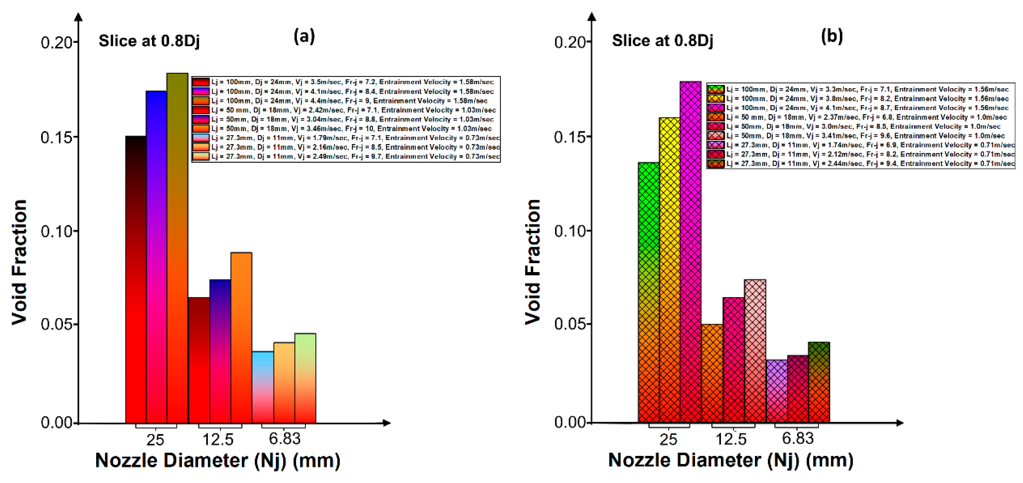
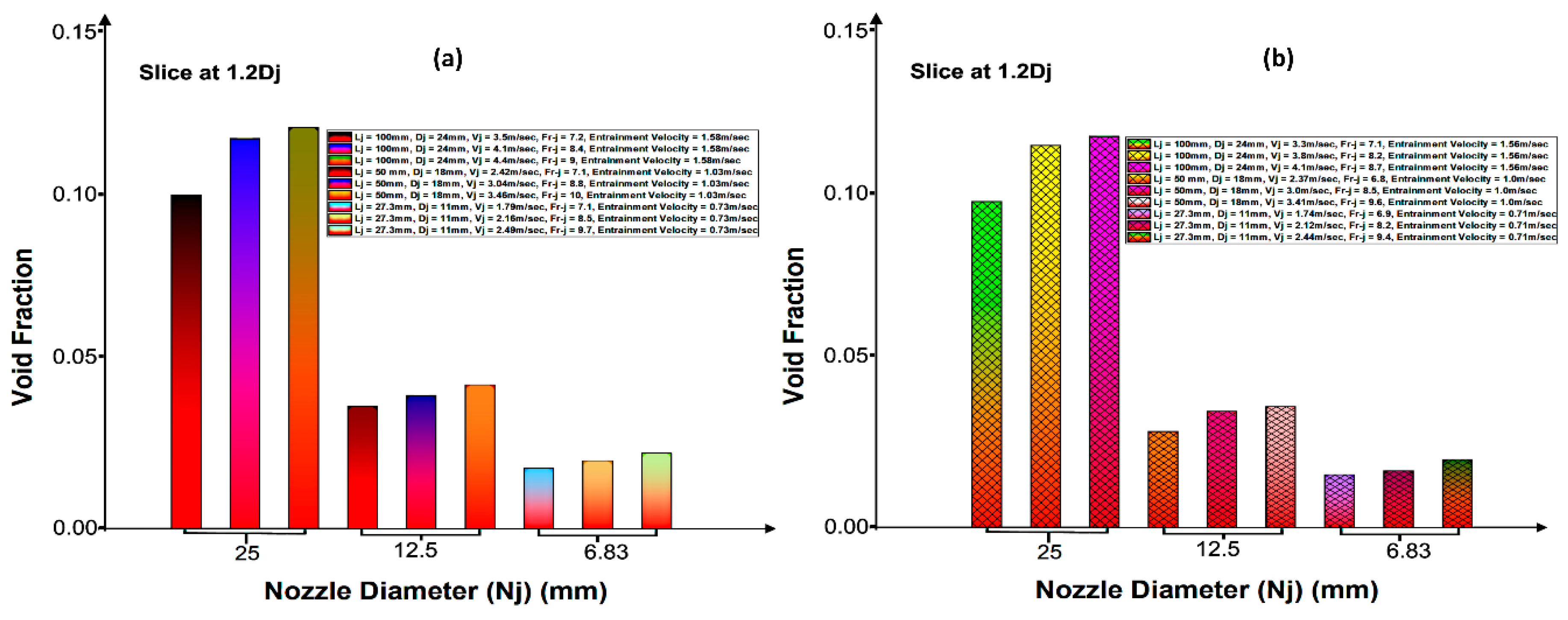
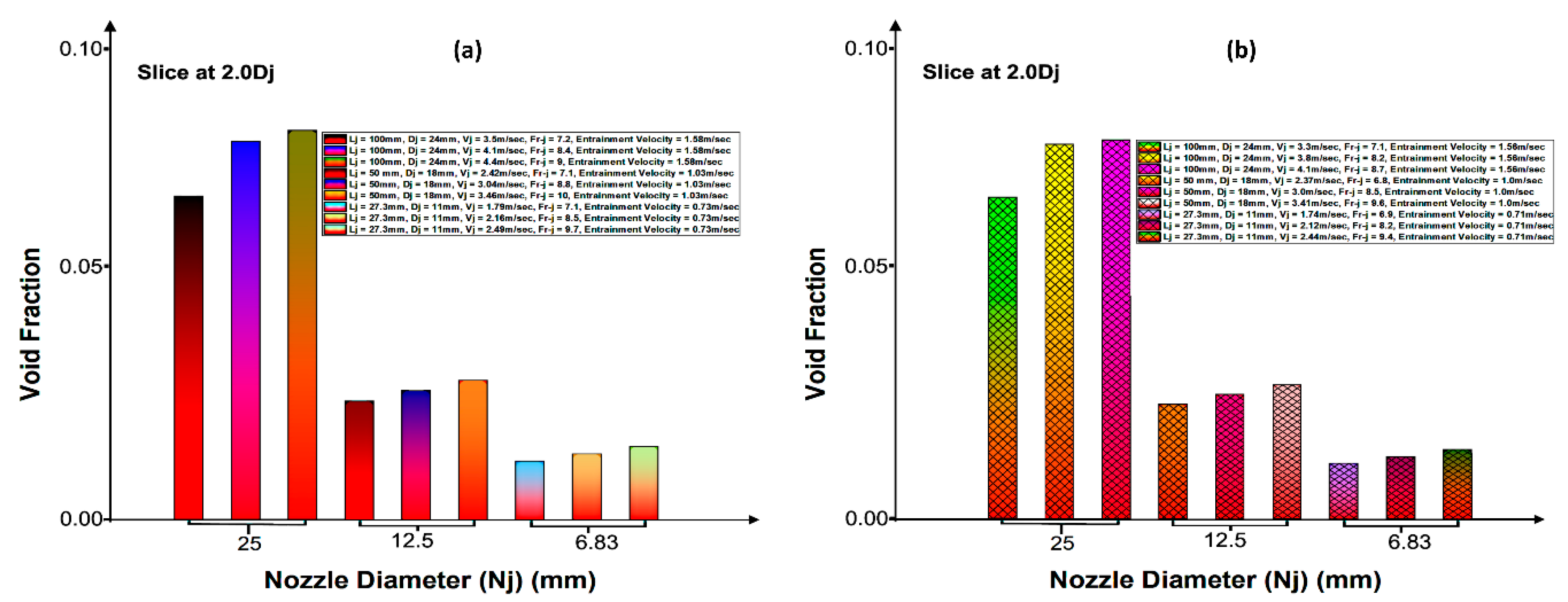
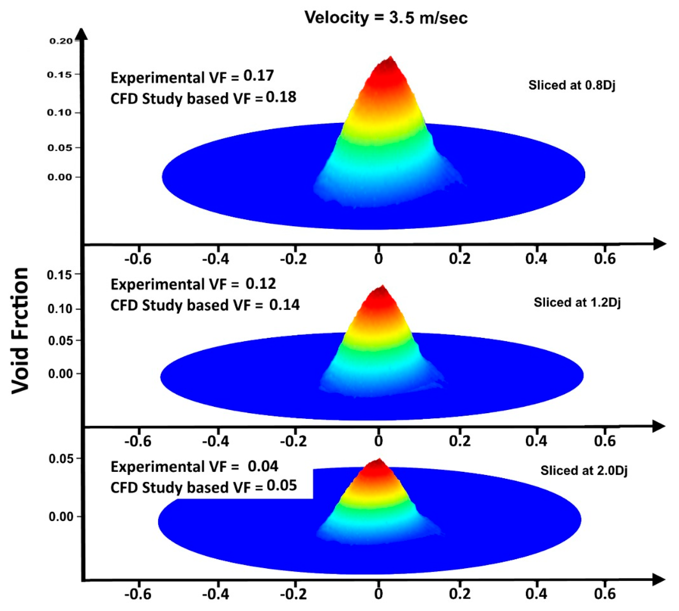
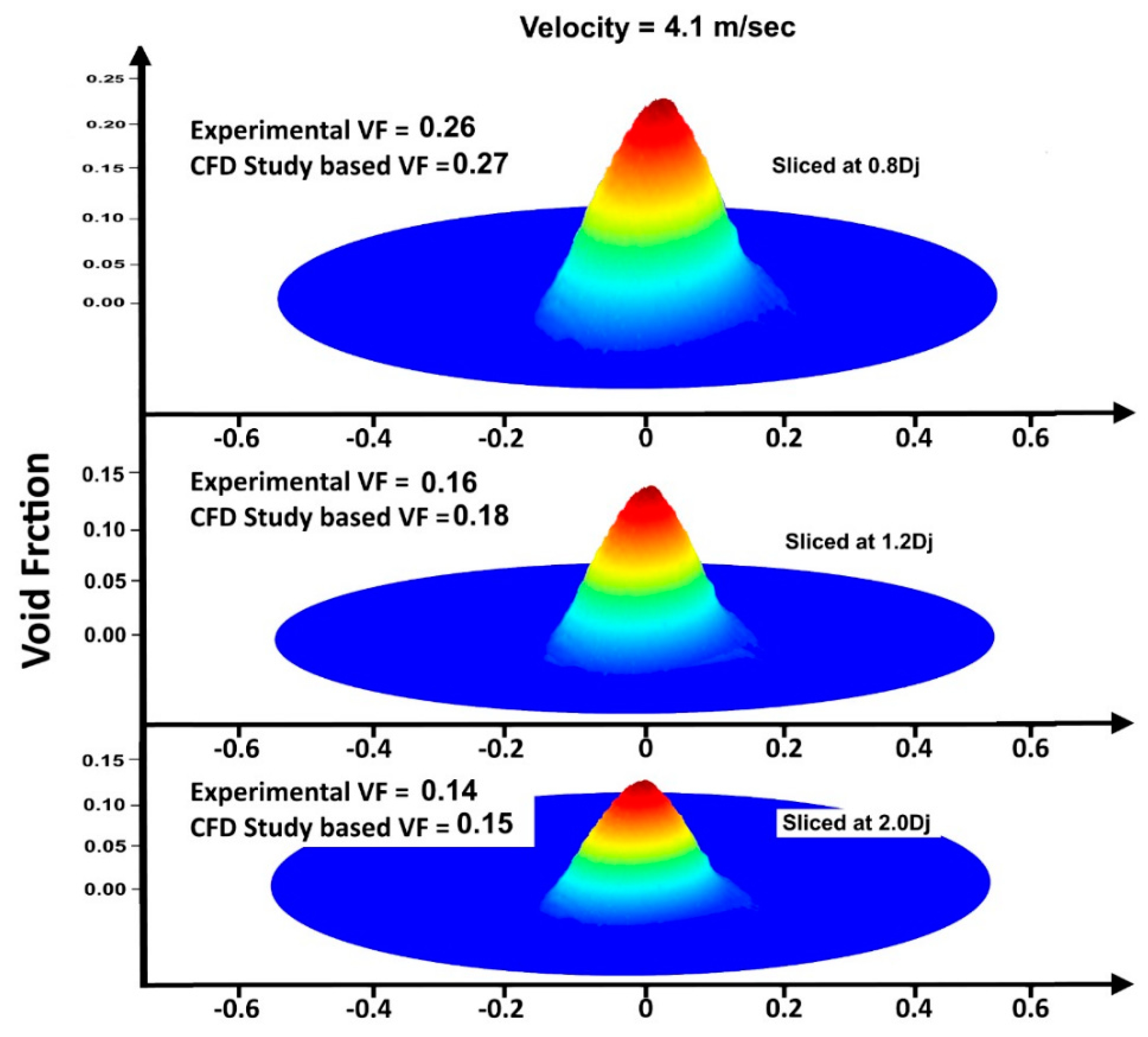
The simulated peaked void fraction along with the depth (0.8D_j, 1.2D_j, and 2.0D_j) from the impact surface along with the corresponding experimental measured values of void fraction are presented in Figure 6, Figure 7 and Figure 8, where the predicted values have been averaged in time. The computed void fraction profiles are obtained for liquid jet velocities of 3.5, 4.1, and 4.4 m/s, to compare both with experimentally measured as well as other simulated void faction profiles.

Figure 9, Figure 10 and Figure 11 provide plots of the numerically and the experimentally obtained void fraction distributions against liquid jet velocities of 3.5, 4.1 and 4.4 m/s at three depths of 0.8, 1.2, and 2.0D_j from the water-free surface, respectively. The bottom profile for all void fraction plots relates to the void fraction distribution obtained at depth 0.8D_j from the contact surface. The simulated void fraction values in this plot agree well with the measured values, and the location of the peaked void fraction matches among the measured value and the present VOF simulation. The peaked void fraction for all three downstream locations (0.8, 1.2 & 2.0D_j) along the depth of the pool from the contact surface is shown in Figure 9, Figure 10 and Figure 11 for the liquid jet velocity of 3.5, 4.1, and 4.4 m/s.

Since the simulated bubbly jet is spreading at depth, 0.8D_j is small, however, the agreement with measurements suggests that the VOF model accurately depicts the location of air entrainment owing to their sources. Further, it can be seen in these figures that the maximum value of the void fraction agrees well with the measured value, which confirms the accuracy of the VOF model in computing the quantity of air that has been entrained.

The plots further down to lower depths from 0.8D_j are presented in Figure 10 and Figure 11, which also indicate good agreement between the experiments and the presented simulations. This indicates that VOF accurately predicts the spreading of bubbly jet and the transport of bubbles which are entrapped by the liquid jet at the impact surface. Transport of bubbles is powered by the liquid velocity along with a balance between turbulent dispersion and drag forces acting on a bubble. Also, the present simulated results make good agreement with the analytical results derived from the simple diffusion scheme adopted by Chanson [39]. Such evidence has been derived by Drew and Passman [47], who have indicated that in circumstances when the dispersed phase momentum under the resulting dominance impact of drag force and turbulent dispersion, the mass conservation should be modeled by a diffusion equation.

Thus, the simulations are obtained at 0.8D_j, 1.2D_j, and 2.0D_j to enable comparison with measured values of the void fraction by Chanson [39] at the same downstream distance from the impact surface. The comparisons between the time-averaged steady simulated values of void fraction and the measured values are presented in Figure 9, Figure 10 and Figure 11.

4. Conclusions

CFD simulations of water jet impacting into a still water pool are performed using the VOF formulation through the commercial code FLUENT, whereas tracing of the interface between air and water is conducted by applying a PLIC algorithm. The simulated results are confirmed by comparing them with Chanson [39] experiments through considering uniformity conditions of experimental three jet sizes along with three jet velocities and three jet diameters. The simulations agreed well with experimental data. Focusing VOF simulations on the developing region of the bubbly plume, it has been inferred that the location of peak void fraction in both experiments and the simulations match. In the experiment, this maximum decays exponentially for deeper locations. However, in the present simulations, it remains almost constant as the two phases move with the same velocity. This fact is inherent to the VOF modeling which resolves only one equation. Hence, no slip velocity between the two phases can be modeled. Slight overestimates of air entrainment rate compared to the experiments of Chanson [39] are noticed for all the three cases, however, VOF simulations came close to the experimental values as compared to the empirical correlation and Euler-Euler scheme. This indicates that the entrainment should be regulated by more parameters than just mere geometric similarities. Hence, small scale-models should be investigated keenly to describe the clear picture of the air entrainment.

References

- Chanson, H. Air Bubble Entrainment in Free-Surface Turbulent Shear Flows; Elsevier: Amsterdam, The Netherlands, 1996. [Google Scholar]
- Chanson, H.; Aoki, S.; Hoque, A. Bubble entrainment and dispersion in plunging jet flows: Freshwater vs. seawater. J. Coast. Res. 2006, 22, 664–677. [Google Scholar] [CrossRef] [Green Version]
- Harby, K.; Chiva, S.; Muñoz-Cobo, J.-L. An experimental study on bubble entrainment and flow characteristics of vertical plunging water jets. Exp. Therm. Fluid Sci. 2014, 57, 207–220. [Google Scholar] [CrossRef]
- Miwa, S.; Yamamoto, Y.; Chiba, G. Research activities on nuclear reactor physics and thermal-hydraulics in Japan after Fukushima-Daiichi accident. J. Nucl. Sci. Technol. 2018, 55, 575–598. [Google Scholar] [CrossRef]
- Kolani, A.R.; Oguz, H.N.; Prosperetti, A. A New Aeration Device. In Proceedings of the ASME Fluids Engineering Summer Meeting, Washington, DC, USA, 21–25 June 1998. [Google Scholar]
- Robison, R. Chicago’s waterfalls. Civ. Eng. N. Y. 1994, 64, 36. [Google Scholar]
- Ohkawa, A.; Kusabiraki, D.; Shiokawa, Y.; Sakai, N.; Fujii, M. Flow and oxygen transfer in a plunging water jet system using inclined short nozzles and performance characteristics of its system in aerobic treatment of wastewater. Biotechnol. Bioeng. 1986, 28, 1845–1856. [Google Scholar] [CrossRef] [PubMed]
- Cummings, P.D.; Chanson, H. Air Entrainment in the Developing Flow Region of Plunging Jets—Part 2: Experimental. ASME J. Fluids Eng. 1997, 119, 603–608. [Google Scholar] [CrossRef] [Green Version]
- Jameson, G.L. Bubbly Flows and the Plunging Jet Flotation Column. In Proceedings of the 12th Australasian Fluid Mechanics Conference, Sydney, Australia, 10–15 December 1995. [Google Scholar]
- Gupta, A.; Yan, D.S. Mineral Processing Design Operations: An Introduction; Elsevier: Amsterdam, The Netherlands, 2016. [Google Scholar]
- Leung, S.M.; Little, J.C.; Holst, T.; Love, N.G. Air/Water Oxygen Transfer in a Biological Aerated Filter. J. Environ. Eng. 2006, 132, 181–189. [Google Scholar] [CrossRef]
- Lorenceau, É.; Quéré, D.; Eggers, J. Air Entrainment by a Viscous Jet Plunging into a Bath. Phys. Rev. Lett. 2004, 93, 254501. [Google Scholar] [CrossRef]
- Biń, A.K. Gas entrainment by plunging liquid jets. Chem. Eng. Sci. 1993, 48, 3585–3630. [Google Scholar] [CrossRef]
- Tojo, K.; Naruko, N.; Miyanami, K. Oxygen transfer and liquid mixing characteristics of plunging jet reactors. Chem. Eng. J. 1982, 25, 107–109. [Google Scholar] [CrossRef]
- McKeogh, E.J.; Ervine, D.A. Air entrainment rate and diffusion pattern of plunging liquid jets. Chem. Eng. Sci. 1981, 36, 1161–1172. [Google Scholar] [CrossRef]
- Bonetto, F.; Lahey, R.T., Jr. An experimental study on air carryunder due to a plunging liquid jet. Int. J. Multiph. Flow 1993, 19, 281–294. [Google Scholar] [CrossRef]
- Zhu, Y.; Hasan, N.; Oğuz, A.P. On the mechanism of air entrainment by liquid jets at a free surface. J. Fluid Mech. 2000, 404, 151–177. [Google Scholar] [CrossRef] [Green Version]
- Qu, X.L.; Khezzar, L.; Danciu, D.; Labois, M.; Lakehal, D. Characterization of plunging liquid jets: A combined experimental and numerical investigation. Int. J. Multiph. Flow 2011, 37, 722–731. [Google Scholar] [CrossRef]
- Ma, J.; Oberai, A.A.; Drew, D.A.; Lahey, R.T. A two-way coupled polydispersed two-fluid model for the simulation of air entrainment beneath a plunging liquid jet. J. Fluids Eng. 2012, 134, 101304. [Google Scholar] [CrossRef]
- Yin, Z.; Jia, Q.; Li, Y.; Wang, Y.; Yang, D. Computational Study of a Vertical Plunging Jet into Still Water. Water 2018, 10, 989. [Google Scholar] [CrossRef] [Green Version]
- Ma, J.; Oberai, A.A.; Drew, D.A.; Lahey, R.T.; Moraga, F.J. A quantitative sub-grid air entrainment model for bubbly flows—Plunging jets. Comput. Fluids 2010, 39, 77–86. [Google Scholar] [CrossRef]
- Mirzaii, I.; Passandideh-Fard, M. Modeling free surface flows in presence of an arbitrary moving object. Int. J. Multiph. Flow 2012, 39, 216–226. [Google Scholar] [CrossRef]
- Elahi, R.; Passandideh-Fard, M.; Javanshir, A. Simulation of liquid sloshing in 2D containers using the volume of fluid method. Ocean Eng. 2015, 96, 226–244. [Google Scholar] [CrossRef]
- van Sint Annaland, M.; Deen, N.G.; Kuipers, J.A.M. Numerical simulation of gas bubbles behaviour using a three-dimensional volume of fluid method. Chem. Eng. Sci. 2005, 60, 2999–3011. [Google Scholar] [CrossRef]
- Boualouache, A.; Kendil, F.Z.; Mataoui, A. Numerical assessment of two phase flow modeling using plunging jet configurations. Chem. Eng. Res. Des. 2017, 128, 248–256. [Google Scholar] [CrossRef]
- Shonibare, O.Y.; Wardle, K.E. Numerical Investigation of Vertical Plunging Jet Using a Hybrid Multifluid–VOF Multiphase CFD Solver. Int. J. Chem. Eng. 2015, 2015, e925639. Available online: https://www.hindawi.com/journals/ijce/2015/925639/ (accessed on 20 March 2020). [CrossRef]
- Hirt, C.W.; Nichols, B.D. Volume of fluid (VOF) method for the dynamics of free boundaries. J. Comput. Phys. 1981, 39, 201–225. [Google Scholar] [CrossRef]
- Julia, J.E.; Ozar, B.; Jeong, J.-J.; Hibiki, T.; Ishii, M. Flow regime development analysis in adiabatic upward two-phase flow in a vertical annulus. Int. J. Heat Fluid Flow 2011, 32, 164–175. [Google Scholar] [CrossRef]
- Lucas, D.; Rzehak, R.; Krepper, E.; Ziegenhein, T.; Liao, Y.; Kriebitzsch, S.; Apanasevich, P. A strategy for the qualification of multi-fluid approaches for nuclear reactor safety. Nucl. Eng. Des. 2016, 299, 2–11. [Google Scholar] [CrossRef]
- Kothe, D.; Rider, W.; Mosso, S.; Brock, J.; Hochstein, J. Volume tracking of interfaces having surface tension in two and three dimensions. In Proceedings of the 34th Aerospace Sciences Meeting and Exhibit, Reno, NV, USA, 15–18 January 1996. [Google Scholar]
- Nguyen, A.V.; Evans, G.M. Computational fluid dynamics modelling of gas jets impinging onto liquid pools. Appl. Math. Model. 2006, 30, 1472–1484. [Google Scholar] [CrossRef] [Green Version]
- Brackbill, J.U.; Kothe, D.B.; Zemach, C. A continuum method for modeling surface tension. J. Comput. Phys. 1992, 100, 335–354. [Google Scholar] [CrossRef]
- Kafka, F.Y.; Dussan, E.B. On the interpretation of dynamic contact angles in capillaries. J. Fluid Mech. 1979, 95, 539–565. [Google Scholar] [CrossRef]
- Boualouache, A.; Zidouni, F.; Mataoui, A. Numerical Visualization of Plunging Water Jet using Volume of Fluid Model. J. Appl. Fluid Mech. 2018, 11, 95–105. [Google Scholar] [CrossRef]
- Gopala, V.R.; van Wachem, B.G. Volume of fluid methods for immiscible-fluid and free-surface flows. Chem. Eng. J. 2008, 141, 204–221. [Google Scholar] [CrossRef]
- Deshpande, S.S.; Trujillo, M.F. Distinguishing features of shallow angle plunging jets. Phys. Fluids 2013, 25, 082103. [Google Scholar] [CrossRef]
- Youngs, D.L. Time-Dependent Multi-Material Flow with Large Fluid Distortion. In Numerical Methods in Fluid Dynamics; Morton, K.W., Baines, M.J., Eds.; Academic Press: Cambridge, MA, USA, 1982; pp. 273–285. [Google Scholar]
- Launder, B.; Spalding, D. The numerical computation of turbulent flows. Comput. Method Appl Mech. Eng. 1974, 3, 269–289. [Google Scholar] [CrossRef]
- Chanson, H.; Aoki, S.; Hoque, A. Physical modelling and similitude of air bubble entrainment at vertical circular plunging jets. Chem. Eng. Sci. 2004, 59, 747–758. [Google Scholar] [CrossRef] [Green Version]
- Iguchi, M.; Okita, K.; Yamamoto, F. Mean velocity and turbulence characteristics of water flow in the bubble dispersion region induced by plunging water jet. Int. J. Multiph. Flow 1998, 24, 523–537. [Google Scholar] [CrossRef]
- Best Practice Guidelines for the Use of CFD in Nuclear Reactor Safety Applications. 2007. Available online: http://inis.iaea.org/Search/search.aspx?orig_q=RN:44037877 (accessed on 15 July 2020).
- Versteeg, H.K.; Weeratunge, M. An Introduction to Computational Fluid Dynamics: The Finite Volume Method; Pearson: London, UK, 2007. [Google Scholar]
- Guyot, G.; Cartellier, A.; Matas, J.-P. Depth of penetration of bubbles entrained by an oscillated plunging water jet. Chem. Eng. Sci. X 2019, 2, 100017. [Google Scholar] [CrossRef]
- Ervine, D.A.; McKeogh, E.; Elsawy, E.M. Effect of turbulence intensity on the rate of air entrainment by plunging water jets. Proc. Inst. Civ. Eng. 1980, 69, 425–445. [Google Scholar] [CrossRef]
- Smith, J.M.; van de Donk, J.A.C. Water Aeration With Plunging Jets. Ph.D. Thesis, Delf University of Technology, Delf, The Netherland, 4 April 1981. [Google Scholar]
- Wilcox, D.C. Turbulence Modeling for CFD; DCW Industries: New York, NY, USA, 1998; Volume 2. [Google Scholar]
- Drew, D.A.; Passman, S.L. Theory of Multicomponent Fluids; Springer Science Business Media: New York, NY, USA, 2006; Volume 135. [Google Scholar]
Figure 1.
A schematic of a vertical plunging jet.
Figure 2.
(a) Real Interface Boundary; (b) Linear Interface Reconstructed Within Each Cell Using PLIC, Following [31].
Figure 3.
(a) Boundary Conditions and Dimensions; (b) Simulation Geometry.
Figure 4.
VOF Sequences of bubbly plume.
Figure 5.
Penetration Length. (a) CFD Study-based Values; (b) Experimental Values.
Figure 6.
(a) VOF Simulated Values; (b) Chanson [39] Measured Values for a Peaked Void Fraction at 0.8Dj Depth.
Figure 7.
(a) VOF Simulated Values; (b) Chanson [39] Measured Values for a Peaked Void Fraction at 1.2Dj Depth.
Figure 8.
(a) VOF Simulated Values; (b) Chanson [39] Measured Values for a Peaked Void Fraction at 2.0Dj Depth.
Figure 9.
VOF Simulated Void Fraction Distribution at 0.8, 1.2 and 2.0Dj for Jet Velocity of 3.5 m/s.
Figure 10.
VOF Simulated Void Fraction Distribution at 0.8, 1.2 and 2.0Dj for Jet Velocity of 4.1 m/s.
Figure 11.
VOF Simulated Void Fraction Distribution at 0.8, 1.2, and 2.0Dj for the Jet Velocity of 4.4 m/s.