Histopathological Imaging–Environment Interactions in Cancer Modeling


1
Department of Biostatistics, Yale University, New Haven, CT 06520, USA
2
SJTU-Yale Joint Center for Biostatistics, Department of Bioinformatics and Biostatistics, School of Life Sciences and Biotechnology, Shanghai Jiao Tong University, Shanghai 200240, China
3
School of Statistics and Management, Shanghai University of Finance and Economics, Shanghai 200433, China
*
Authors to whom correspondence should be addressed.
Cancers 2019, 11(4), 579; https://doi.org/10.3390/cancers11040579
Submission received: 26 February 2019
/
Revised: 17 April 2019
/
Accepted: 19 April 2019
/
Published: 24 April 2019
(This article belongs to the Special Issue Application of Bioinformatics in Cancers)
Abstract
:Histopathological imaging has been routinely conducted in cancer diagnosis and recently used for modeling other cancer outcomes/phenotypes such as prognosis. Clinical/environmental factors have long been extensively used in cancer modeling. However, there is still a lack of study exploring possible interactions of histopathological imaging features and clinical/environmental risk factors in cancer modeling. In this article, we explore such a possibility and conduct both marginal and joint interaction analysis. Novel statistical methods, which are “borrowed” from gene–environment interaction analysis, are employed. Analysis of The Cancer Genome Atlas (TCGA) lung adenocarcinoma (LUAD) data is conducted. More specifically, we examine a biomarker of lung function as well as overall survival. Possible interaction effects are identified. Overall, this study can suggest an alternative way of cancer modeling that innovatively combines histopathological imaging and clinical/environmental data.
1. Introduction
Cancer is extremely complex. Extensive statistical investigations have been conducted, modeling various cancer outcomes/phenotypes. A long array of measurements from different domains have been used in cancer modeling, including clinical/environmental factors, socioeconomic factors, omics (genetic, genomic, epigenetic, proteomic, etc.) measurements, histopathological imaging features, and others. However, none of the existing models is completely satisfactory, and it remains a challenging task to develop new ways of cancer modeling.
Imaging has been playing an irreplaceable role in cancer practice and research [1]. It is routine for radiologists to use Computed Tomography (CT), Magnetic Resonance Imaging (MRI), Positron Emission Computed Tomography (PET), and other techniques to generate radiological images, which can inform the size, location, and other “macro” features of tumors [2]. Biopsies are ordered, and pathologists review the slides of representative sections of tissues to make definitive diagnosis. This procedure generates histopathological (diagnostic) images [3]. Through microscopically examining small pieces of tissues, more “micro” features of tumors are obtained. Histopathological images have been used as the gold standard for diagnosis. More recently, histopathological imaging features have also been used to model other cancer outcomes/phenotypes. For example, in [4], they were used for predicting the prognosis of estrogen receptor-negative breast cancer, and a multivariate Cox regression was adopted. In [5], histopathological imaging features were used in a k-nearest neighbor classifier to assign images into different groups of Gleason tumor grading for prostate cancer patients.
With the complexity of cancer, a single domain of measurement is insufficient, and measurements from multiple sources are needed in modeling [6]. In the literature, histopathological imaging features and clinical/environmental risk factors have been combined in an additive manner for modeling cancer outcomes. In [7], for modeling lung cancer prognosis, clinical factors (including age, gender, cancer type, smoking history, and tumor stage) were combined with imaging features in a multivariate Cox regression model. This study and those alike have shown that combining the two sources of information are more informative than a single source. Our literature review suggests that most if not all of the existing studies have considered the additive effects of histopathological imaging features and clinical/environmental factors, and studies that accommodate their interactions (referred to as “I–E” interactions, with “I” and “E” standing for imaging and clinical/environmental factors, in this study) are lacking. Statistically, adding interactions when the main-effect models are not fully satisfactory is “normal”. Biologically speaking, incorporating such interactions have been partly motivated by the success of gene–environment (G–E) interactions. Specifically, in the literature, the biological rationale and practical success of G–E interactions have been well established [8]. Cancer is a genetic disease. Histopathological images reflect essential information on the histological organization and morphological characteristics of tumor cells and their surrounding tumor microenvironment, which are heavily regulated by tumors’ molecular features. As such, from G–E interactions, we may naturally derive I–E interactions. It is noted that I–E and G–E interaction analyses cannot replace each other. More specifically, not all genetic information is contained in imaging features, and histopathological features, as reflected in imaging data, are also affected by factors other than molecular changes.
This study has also been partly motivated by the ineffectiveness of techniques adopted in the existing studies. Histopathological images contain rich information, and the number of extracted features can be quite large, posing analytic challenges. This dimension problem is “brutally” handled in some studies. For example, in [9], the univariate Cox model was fit to each imaging feature, and those with the strongest marginal effects were selected. Such features were then used along with clinical characteristics, including age, gender, smoking status, and tumor stage, to construct the final prognostic model. When joint modeling is the ultimate goal, the aforementioned approach may miss truly important signals in the first step of screening. To accommodate the high dimensionality in joint modeling, penalization and other regularization techniques have been adopted. For example, in [10], the elastic net approach, which combines the Lasso and ridge penalties, was used along with Cox regression. With the differences between interactions and main effects, such methods cannot be directly applied to analysis that accommodates I–E interactions. There are also studies that use advanced deep learning techniques. For example, Bychkov and others [11] used the CNN (convolutional neural network) technique to predict colorectal cancer prognosis based on images of tumor tissue samples. Other examples also include [12,13]. Such deep learning techniques may excel in prediction, however, usually lack interpretations and also suffer from a lack of stability when sample size is small.
The main objective of this article is to explore accommodating I–E interactions in cancer modeling. Although the concept may seem simple, such an interaction analysis has not been conducted in the literature. The adopted statistical methods have been “borrowed” from G–E interaction analysis. With the connectedness between genetic and histopathological imaging features and parallelization of G–E and I–E interaction analysis, such a strategy is sensible. The proposed interaction analysis strategy and methods are demonstrated using the The Cancer Genome Atlas (TCGA) lung adenocarcinoma data. Overall, this study may suggest an alternative way of utilizing histopathological imaging data and modeling cancer more accurately.
2. Data
We demonstrate I–E interaction analysis using the TCGA lung cancer data. TCGA is a collective effort organized by lNational Cancer Institute (NCI) and has published comprehensive data, especially on outcomes/phenotypes, clinical/environmental measures, and histopathological images, for lung and other cancer types. Lung cancer is the leading cause of cancer death globally [14], and lung adenocarcinoma (LUAD) is the most common histological subtype and has posed increasing public concerns [15]. The TCGA LUAD data has been analyzed in multiple published studies, including [7,9], who analyzed histopathological images, and [16,17], who conducted analysis on clinical/environmental factors. Thus, it is of interest to “continue” these studies on main additive effects and further examine potential I–E interactions with the TCGA LUAD data. It also has the advantage of having a relatively larger sample size, which is critical to achieve meaningful findings. It is noted that the proposed analysis can be directly applied to data on other cancer types.
We acquire 541 whole slide histopathology images from the TCGA ldata portal [18]. To extract imaging features, we adopt the following pipeline developed by Luo and others [9]. First, as the size of the whole slide images, which is from 300 Mb up to 2 Gb with 110,000 × 70,000 pixels, is too huge to be analyzed directly, each image is cropped into sub-images with 500 × 500 pixels and saved as tiff image files using the Openslide Python library. Analyzing all the sub-images (more than 10 million image tiles in total) is still computationally unfeasible. Thus, twenty representative tiff sub-images that contain mostly (>50%) regions of interest are randomly selected as input for the following process. It is expected that the randomly selected sub-images are representative samples for the overall “population” of sub-images. Such cropping and random selection are common steps in whole slide image processing and widely adopted in published imaging studies [10,19,20,21]. It is noted that randomly selecting sub-images may lead to imaging features with very small differences (and so affect downstream analysis). However, as our main goal is cancer model building, as opposed to feature selection, such small differences may not be of major concern.
Second, we adopt CellProfiler [22], a platform designed for cell image processing and used in quite a few recent publications, to extract quantitative features from each sub-image. Specifically, image colors are separated based on hematoxylin and eosin staining, and converted to grayscale for extracting regional features. Next, cell nuclei are detected and segmented so that cell-level features can be specifically measured. Other features such as regional occupation, area fraction, and neighboring architecture are also captured. Irrelevant features such as file size and execution information are excluded from analysis. This procedure results in a total of 772 features which are categorized into the texture, geometry, and holistic groups. Specifically, the texture group contains Haralick, Gabor “wavelet”, and Granularity features, which are classic image processing features, measure the texture properties of cells and tissues, and have been examined in a large number of imaging studies. The geometry group contains features that describe the geometry properties (such as area, perimeter, and so on), and those extracted by Zernike moments. The holistic group contains holistic statistics that describe overall information, such as the total area, perimeter and number of nuclei, and nuclear staining area fraction.
Third, for each patient, the features of images are normalized using sample mean at the patient level. Missing values (with a missing rate lower than 20%) are imputed using sample medians.
For clinical/environmental risk factors, we consider age, American Joint Committee on Cancer tumor pathologic stage, tobacco smoking history indicator, and sex. These variables have been suggested as associated with multiple lung cancer outcomes/phenotypes, including those analyzed in this article [23]. In particular, Nordquis and others [24] found that the mean age at diagnosis of lung adenocarcinoma among never-smokers was significantly higher than that among current smokers, and the never-smokers with lung adenocarcinoma were predominantly female. Studies have shown that tobacco smoking is responsible for 90% of lung cancer [25], and has been identified as a negative prognostic factor for lung adenocarcinoma [26]. In addition, these factors have also been considered in G–E interaction analysis [27].
Multiple outcome variables have been analyzed in the literature [7]. In this article, we consider two important response variables: (a) FEV1: the reference value for the pre-bronchodilator forced expiratory volume in one second in percent. It is an important biomarker for lung capacity. It is continuously distributed, with mean 80.28 and interquartile range [67.00, 96.25]. Data is available for 132 subjects; and (b) overall survival, which is subject to right censoring. Data is available for 271 subjects, among whom 102 died during follow-up. The mean observed time is 27.47 months, with interquartile range [14.06, 35.00].
The adopted feature extraction process follows [9], where the extracted imaging features were used to predict lung cancer prognosis. Similar processes have also been adopted in other publications [10,19]. Different from limited histopathological features recognized visually by pathologists, CellProfiler extracted features are morphological features of tissue texture, cells, nuclei, and neighboring architecture. These features are extracted and measured by comprehensive computer algorithms, and are impossible to be assessed by human eyes. As demonstrated in [9], quantitative imaging features provide objective and rich information contained in images that can reveal hidden information to decode tumor development and progression in lung cancer. Following the literature [9,20,21], we adopt feature names automatically assigned by CellProfiler, as can be partly seen in Table 1, Table 2, Table 3 and Table 4. These names provide a brief description of the extracted information with the general form “Compartment_FeatureGroup_Feature_Channel_Parameters”. For example, features “AreaShape_MedianRadius” and “AreaShape_MaximumRadius” measure the median and maximum radius of the identified tissue, respectively. As in some recent studies [9,20,21], in this study, our goal is not to identify specific imaging features as markers and make biological interpretations. Instead, we aim to conduct better cancer modeling by incorporating I–E interactions. As such, although they may not have simple, explicit biological interpretations, these features are sensible for our analysis.
3. Methods
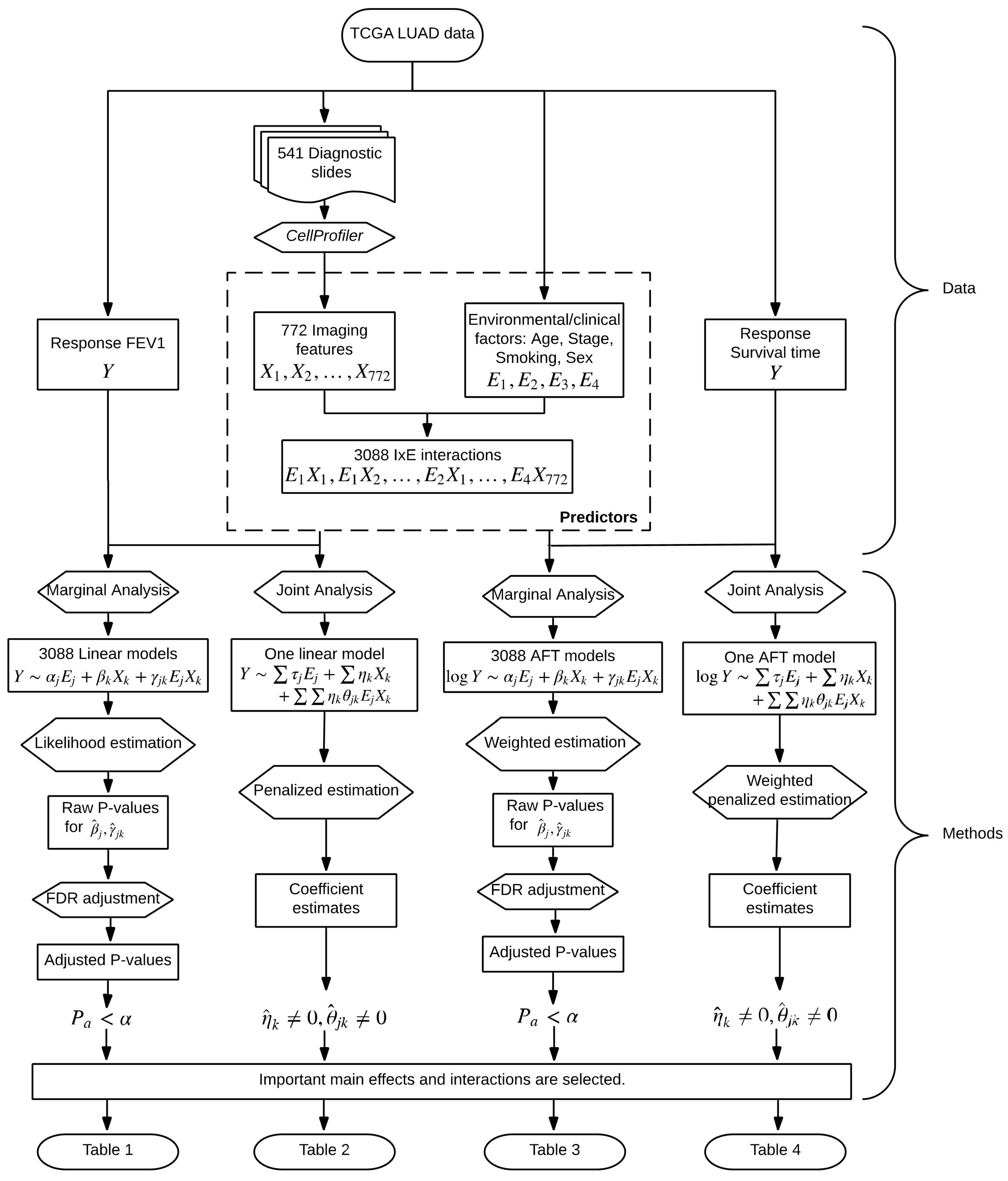
In parallel to G–E interaction analysis [28], we conduct two types of I–E interaction analysis, namely marginal and joint analysis. The overall flowchart of analysis is provided in Figure 1. In marginal analysis, one imaging feature, one clinical/environmental variable (or multiple such variables), and their interaction are analyzed at a time. In joint analysis, all imaging features, all clinical/environmental variables, and their interactions are analyzed in a single model. The two types of analysis have their own pros and cons and cannot replace each other. We refer to the literature [29,30] for more detailed discussions on the two types of analysis.
First, consider a continuous cancer outcome, which matches the FEV1 analysis. Denote Y as the length N vector of outcome, where N is the sample size. Denote E = [E1, ⋯, EJ] as the N × J matrix of clinical/environmental variables, and X = [X1, ⋯, XK] as the N × K matrix of imaging features. As represented by the LUAD data, usually clinical/environmental variables are pre-selected and low-dimensional, and imaging features are high-dimensional.
3.1. Marginal Analysis
Detailed discussions of marginal G–E interaction analysis are available in [31] and other recent literature. The marginal I–E interaction analysis proceeds as follows. First, assume that Y, E, and X have been properly centered.
- (a)
- For and , consider the linear regression modelwhere and respectively represent the main effects of the jth clinical/environmental factor and the kth imaging feature, is the interactive effect, and ϵ is the random error. A total of J × K models are built.
- (b)
- As each model has a low dimension, estimates can be obtained using standard likelihood based approaches and existing software. p-values can be obtained accordingly.
- (c)
- Interactions (and main effects) with small p-values are identified as important. When more definitive conclusions are needed, the false discovery rate (FDR) or Bonferroni approach can be applied.
It is noted that, in Step (a), one clinical/environmental variable is analyzed in each model, which follows [31]. It is also possible to accommodate all clinical/environmental variables in each model. In Step (c), discoveries can be made on interactions only or interactions and main effects combined. Advantages of marginal analysis include its computational simplicity and stability. On the negative side, with the complexity of cancer, an outcome/phenotype is usually associated with multiple imaging features and clinical/environmental variables. As such, each marginal model can be “mis-specified” or “suboptimal”. In addition, there is a lack of attention to the differences between interactions and main effects.
3.2. Joint Analysis
Joint analysis can tackle some limitations of marginal analysis, and is getting increasingly popular in statistical and bioinformatics literature. It proceeds as follows.
- (a)
- Consider the joint modelwhere and are the main effects of the jth environmental factor and the kth imaging feature, respectively, and the product of and corresponds to the interaction.
- (b)
- For estimation, consider the Lasso penalizationwhere , and are tuning parameters. In numerical study, we select the tuning parameters using the extended Bayesian information criterion [32].
- (c)
- Interactions (and main effects) with nonzero estimates are identified as being associated with the outcome.
3.3. Accommodating Survival Outcomes
Consider cancer survival. Denote T as the N-vector of survival times. Below, we describe joint analysis, and marginal analysis can be conducted accordingly. We adopt the AFT (accelerated failure time) model, under which
where notations have similar implications as in the above section. With high-dimensional data, the AFT model has been widely adopted because of its lucid interpretation and more importantly computational simplicity [33]. Under right censoring, denote C as the N-vector of censoring times, Y = log(min(T, C)), and δ = I(T ≤ C), where operations are taken component-wise. To accommodate censoring, a weighted approach is adopted. Assume that data have been sorted according to Yi’s from the smallest to the largest. The Kaplan–Meier weights can be computed as , , . Similar to Equation (3), consider the penalized estimation
where the square root and multiplication are taken component-wise. Interpretations and other operations are the same as for continuous outcomes.
In joint analysis, the most prominent challenge is the high dimensionality. Here, the penalization technique is adopted, which can simultaneously accommodate high dimensionality and identify relevant interactions/main effects. Another feature of this analysis that is worth highlighting is that it respects the “main effects, interactions” hierarchy. That is, if an I–E interaction is identified, the corresponding main imaging feature effect is automatically identified. It has been suggested that, statistically and biologically, it is critical to respect this hierarchy [34]. We refer to the literature [35,36] for alternative penalization and other joint interaction analysis methods. Compared to marginal analysis, joint analysis can be computationally more challenging, and well-developed software packages are still limited. In addition, the analysis results can be less stable.
The proposed analysis can be effectively realized. To facilitate data analysis within and beyond this study, we have developed R code and made it publicly available at www.github.com/shuanggema.
4. Results
4.1. Analysis of FEV1
4.1.1. Marginal Analysis
After the FDR adjustment, none of the main effects or interactions are statistically significant. In Table 1, we present the main effects and interactions with the smallest (unadjusted) p-values. The top ranked main effects are from the Geometry and Texture groups, and the top ranked interactions are from the Geometry group and with sex.
Based on the analysis results, we conduct a power calculation. First, assume the current levels of estimated effects and their variations. Then, with a sample size of 224, the top ranked I–E interactions can be identified as significant with target FDR 0.1. Second, consider the current sample size and levels of variations. Then, an effect of −0.35 can be identified as significant with target FDR 0.1.
For comparison, we conduct the analysis of main effects (without interactions). The top eight main effects (with the smallest p-values) have four overlaps with those in Table 1, suggesting that accommodating interactions can lead to different findings.
4.1.2. Joint Analysis
The analysis results are provided in Table 2. A total of 11 imaging features are identified, representing the Geometry and Texture groups. A total of 11 interactions are identified, with all four clinical/environmental variables.
For comparison, we consider the joint model with all clinical/environmental variables and imaging features but no interactions. Lasso penalization is applied for selection and estimation. A total of eight imaging features are identified, with one overlapping with those in Table 2. We further compute the RV coefficient, which may more objectively quantify the amount of “overlapping information” between two analyses. Specifically, it measures the “correlation” between two data matrices of important effects identified by two different approaches, with a larger value indicating higher similarity. The RV coefficient is 0.24, suggesting a mild level of overlapping.
A significant advantage of joint analysis is that it can lead to a predictive model for the outcome variable. We conduct the evaluation of prediction based on a resampling procedure, which may provide support to the validity of analysis. Specifically, we split data into a training and a testing set, generate estimates using the training data, and make predictions for the testing set subjects. The PMSE (prediction mean squared error) is then computed. This procedure is repeated 100 times, and the mean PMSE is computed. The I–E interaction model has a mean PMSE of 0.84, whereas the main-effect-only model has a mean PMSE of 1.12. This significant improvement suggests the benefit of accommodating interactions.
4.2. Analysis of Overall Survival
4.2.1. Marginal Analysis
The analysis results are provided in Table 3, where we present estimates, raw p-values, as well as the FDR adjusted p-values. Three imaging features from the Holistic group have the FDR adjusted p-values < 0.1. In addition, 36 imaging features from the Geometry group and 24 features from the Texture group are identified as having interactions with Smoking, the most important environmental factor for lung cancer. Compared to the above analysis, more “signals” are identified. Note that the effective sample size is smaller than that above. As such, the smaller p-values are likely to be caused by stronger signals.
For comparison, we conduct the analysis of main effects. One imaging feature is identified as having FDR adjusted p-value < 0.1, which is also identified in Table 3. With the complexity of lung cancer prognosis, the interaction analysis, which identifies more effects, can be more sensible.
4.2.2. Joint Analysis
The analysis results are provided in Table 4. A total of 31 imaging features are identified, representing the three feature groups. Two imaging features are identified as interacting with two and four clinical/environmental variables, respectively.
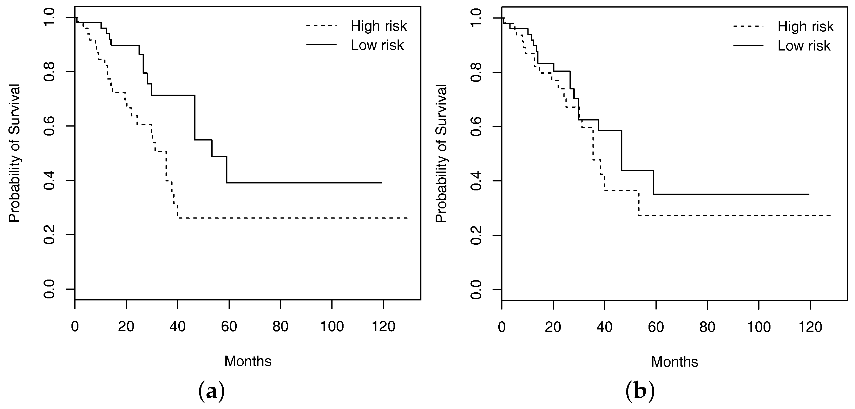
The analysis of main effects is conducted using the Lasso penalization. A total of two imaging features are identified, with one overlapping with those in Table 4. The RV coefficient is computed as 0.40, representing a moderate level of overlapping. As with FEV1, prediction evaluation is also conducted based on resampling. For the testing set, subjects are classified into low and high risk groups with equal sizes based on the predicted survival times, where subjects with predicted survival times larger than the median are classified into the low risk group. For one resampling of training and testing sets, in Figure 2, we plot the Kaplan–Meier curves estimated using the observed survival times for the predicted low and high risk groups, along with those generated under the additive main-effect model. Compared to the main-effect model, it is obvious that the two risk groups identified by the I–E interaction model have a much clearer separation of the survival functions, indicating better prediction performance. To be more rigorous, we further conduct a logrank test, which is a nonparametric test for comparing the survival distributions of two subject groups. With 100 resamplings, the average logrank statistics are 7.28 (I–E interaction model, p-value = 0.007) and 0.99 (main-effect model, p-value = 0.320), respectively. The superior prediction performance of the I–E interaction models suggests that incorporating interactions can lead to clinically more powerful models, justifying the value of the proposed analysis.
4.3. Simulation
Comparatively, joint analysis is newer and has been less conducted. To gain more insights into the validity of findings from our joint interaction analysis, we conduct a set of data-based simulation. Specifically, the observed imaging features and clinical/environmental factors are used. To generate variations across simulation replicates, we use resampling, with sample sizes set as 200. The “signals” and their levels are set as those in Table 2 and Table 4, respectively. For both the continuous and (log) survival outcomes, we generate random errors from N(0, 1). For the survival setting, we generate the censoring times from randomly sampling the observed. The Lasso-based penalization approach is then applied, with tuning parameters selected using the extended Bayesian information criterion (BIC) approach. To evaluate identification, TP (true positive) and FP (false positive) values are computed. Summary statistics are computed based on 100 replicates. Under the continuous outcome setting, there are 11 true main effects and 11 I–E interactions. For main effects, the TP and FP values are 9.75 (1.65) and 3.15 (1.39), respectively, where numbers in “()” are standard deviations. For interactions, the TP and FP values are 7.35 (0.99) and 0.05 (0.22), respectively. Under the censored survival outcome setting, there are 31 true main effects and 6 I–E interactions. For main effects, the TP and FP values are 24.41 (3.98) and 13.90 (2.47), respectively. For interactions, the TP and FP values are 3.24 (0.21) and 0.24 (0.12), respectively. Overall, at the estimated signal levels and with the observed feature distributions, the joint analysis is capable of identifying the majority of true interactions and main effects, with a moderate number of false discoveries. This provides a high level of confidence to the joint interaction analysis.
5. Discussion
Histopathological imaging analysis has been routine in cancer diagnosis, and recently, its application in the analysis of cancer biomarkers, outcomes, and phenotypes has been explored. This study has taken a natural next step and conducted the imaging-environment interaction analysis. Statistically and biologically speaking, the analysis has been partly motivated by G–E interaction analysis. It is noted that the statistical methods themselves have been almost fully “translated” from G–E interaction analysis. As I–E interaction analysis has not been conducted in published cancer modeling studies, it is sensible to first employ well-developed methods, and in the future, methods that are more tailored to imaging data may be developed. We also note that in cancer modeling and other biomedical fields, it is not uncommon to apply methods well developed in one field to other new fields. The proposed I–E interaction analysis, especially joint analysis, may seem considerably more complex than some cancer modeling approaches. With the complexity of cancer, models with a few variables and simple statistical analysis are getting increasingly insufficient. Published studies have suggested that advanced statistical techniques and complex models are needed. Recent developments for lung cancer, including the elastic net-Cox analysis [10], deep convolutional neural network [13], and deep network based on convolutional and recurrent architectures [11], have comparable or higher levels of complexity compared to the proposed analysis. Artificial intelligence (AI) techniques, which have been recently used for cancer modeling in particular including the radiomics analysis of non-small-cell lung cancer [37,38], have even higher levels of complexity. We conjecture that such complexity will also be needed for future developments in cancer modeling using imaging data. The increasing complexity in cancer modeling seems to be an inevitable trend, and domain specific expertise is a must for such analysis.
We have analyzed the TCGA LUAD data with a continuous and a censored survival outcome. This choice has been motivated by the clinical importance of lung adenocarcinoma as well as data availability (a larger sample size). It is noted that the proposed analysis and R program will be directly applicable to the analysis of data on other cancer types. I–E interactions have been identified in both marginal and joint analysis, for both FEV1 and overall survival. There is one prominent difference between imaging and genetic/clinical data. With extensive investigations and functional experiments, the biological and biomedical implications of most clinical/environmental factors and genes are at least partially known. It is thus possible to evaluate whether G–E interactions are biologically sensible. The circumstance is significantly different for histopathological imaging features. The rationale and algorithms for feature extraction have been made clear in the developments of CellProfiler and other software. However, the identified features do not have lucid biological interpretations. As such, we are not able to objectively assess the biological implications of the findings in Table 1, Table 2, Table 3 and Table 4. It is noted that this limitation is also shared by recently published imaging studies [9,20,21], which have unambiguously demonstrated the great value of such imaging features in cancer modeling. It is also noted that imaging features derived from computer-aided pathological analysis have the unique advantage of being objective and comprehensive, and can reveal hidden information contained in histopathological images that cannot be recognized or assessed by pathologists. Our statistical evaluations, including the prediction evaluation and data-based simulation, can provide support to the analysis results to a great extent. In general, more investigations into the biological implications of the computer-program-extracted imaging features will be needed.
This study has suggested a new venue for cancer modeling. Although findings made on LUAD may not be applicable to other cancers, the analysis technique and R program will be broadly applicable. Following the flowchart in Figure 1 and detailed steps described in this article, and using the publicly available R program, cancer biostatisticians and clinicians should be able to carry out the proposed analysis with their own data. More specifically, with their own clinical/environmental and imaging data, they will be able to construct models for prognosis and other outcomes/phenotypes. Such models, as other cancer models (for example those using omics data), can be used to assist clinical decision making. Overall, this study may help advance the challenging field of cancer modeling.
6. Conclusions
Histopathological imaging data may harbor important information on cancer and has been recently used for modeling cancer clinical outcomes and phenotypes. This study has been the first to examine the interactions between imaging features and clinical/environmental risk factors in cancer modeling. Marginal and joint analysis approaches have been described. In the analysis of TCGA LUAD data, it has been shown that I–E interactions may be important for modeling FEV1 and overall survival. Overall, this study has suggested a new paradigm of cancer bioinformatics modeling.
Author Contributions
All authors contributed to conceptualization, methodology, and writing. T.Z. conducted data processing. Y.X. performed data analysis and simulation.
Funding
This work was supported by the NIH (R01CA204120, P50CA196530); the Yale Cancer Center Pilot Award; the National Natural Science Foundation of China (91546202, 71331006); and the Bureau of Statistics of China (2018LD02).
Acknowledgments
We thank the editor and reviewers for their careful review and insightful comments, which have led to a significant improvement of this article.
Conflicts of Interest
The authors declare no conflict of interest.
References
- Fass, L. Imaging and cancer: A review. Mol. Oncol. 2008, 2, 115–152. [Google Scholar] [CrossRef] [Green Version]
- Benzaquen, J.; Boutros, J.; Marquette, C.; Delingette, H.; Hofman, P. Lung cancer screening, towards a multidimensional approach: Why and how? Cancers 2019, 11, 212. [Google Scholar] [CrossRef]
- Gurcan, M.N.; Boucheron, L.; Can, A.; Madabhushi, A.; Rajpoot, N.; Yener, B. Histopathological image analysis: A review. IEEE Rev. Biomed. Eng. 2009, 2, 147–171. [Google Scholar] [CrossRef] [PubMed]
- Yuan, Y.; Failmezger, H.; Rueda, O.M.; Ali, H.R.; Gräf, S.; Chin, S.F.; Schwarz, R.F.; Curtis, C.; Dunning, M.J.; Bardwell, H.; et al. Quantitative image analysis of cellular heterogeneity in breast tumors complements genomic profiling. Sci. Transl. Med. 2012, 4, 157ra143. [Google Scholar] [CrossRef]
- Tabesh, A.; Teverovskiy, M.; Pang, H.Y.; Kumar, V.P.; Verbel, D.; Kotsianti, A.; Saidi, O. Multifeature prostate cancer diagnosis and Gleason grading of histological images. IEEE Trans. Med. Imaging 2007, 26, 1366–1378. [Google Scholar] [CrossRef]
- Zhong, T.; Wu, M.; Ma, S. Examination of independent prognostic power of gene expressions and histopathological imaging features in cancer. Cancers 2019, 11, 361. [Google Scholar] [CrossRef] [PubMed]
- Wang, H.; Xing, F.; Su, H.; Stromberg, A.; Yang, L. Novel image markers for non-small cell lung cancer classification and survival prediction. BMC Bioinform. 2014, 15, 310. [Google Scholar] [CrossRef]
- Hunter, D.J. Gene–environment interactions in human diseases. Nat. Rev. Genet. 2005, 6, 287–298. [Google Scholar] [CrossRef]
- Luo, X.; Zang, X.; Yang, L.; Huang, J.; Liang, F.; Rodriguez-Canales, J.; Wistuba, I.I.; Gazdar, A.; Xie, Y.; Xiao, G. Comprehensive computational pathological image analysis predicts lung cancer prognosis. J. Thorac. Oncol. 2017, 12, 501–509. [Google Scholar] [CrossRef]
- Yu, K.H.; Zhang, C.; Berry, G.J.; Altman, R.B.; Ré, C.; Rubin, D.L.; Snyder, M. Predicting non-small cell lung cancer prognosis by fully automated microscopic pathology image features. Nat. Commun. 2016, 7, 12474. [Google Scholar] [CrossRef] [PubMed] [Green Version]
- Bychkov, D.; Linder, N.; Turkki, R.; Nordling, S.; Kovanen, P.E.; Verrill, C.; Walliander, M.; Lundin, M.; Haglund, C.; Lundin, J. Deep learning based tissue analysis predicts outcome in colorectal cancer. Sci. Rep. 2018, 8, 3395. [Google Scholar] [CrossRef] [PubMed]
- Zhu, X.; Yao, J.; Zhu, F.; Huang, J. Wsisa: Making survival prediction from whole slide histopathological images. In Proceedings of the IEEE Conference on Computer Vision and Pattern Recognition, Honolulu, HI, USA, 21–26 July 2017; pp. 7234–7242. [Google Scholar]
- Coudray, N.; Ocampo, P.S.; Sakellaropoulos, T.; Narula, N.; Snuderl, M.; Fenyö, D.; Moreira, A.L.; Razavian, N.; Tsirigos, A. Classification and mutation prediction from non–small cell lung cancer histopathology images using deep learning. Nat. Med. 2018, 24, 1559–1567. [Google Scholar] [CrossRef]
- Boolell, V.; Alamgeer, M.; Watkins, D.; Ganju, V. The evolution of therapies in non-small cell lung cancer. Cancers 2015, 7, 1815–1846. [Google Scholar] [CrossRef] [PubMed]
- Cancer Genome Atlas Research Network. Comprehensive molecular profiling of lung adenocarcinoma. Nature 2014, 511, 543–550. [Google Scholar] [CrossRef] [PubMed] [Green Version]
- Karlsson, A.; Ringner, M.; Lauss, M.; Botling, J.; Micke, P.; Planck, M.; Staaf, J. Genomic and transcriptional alterations in lung adenocarcinoma in relation to smoking history. Clin. Cancer Res. 2014, 20, 4912–4924. [Google Scholar] [CrossRef]
- Li, X.; Shi, Y.; Yin, Z.; Xue, X.; Zhou, B. An eight-miRNA signature as a potential biomarker for predicting survival in lung adenocarcinoma. J. Transl. Med. 2014, 12, 159. [Google Scholar] [CrossRef]
- The Cancer Genome Atlas Data Portal Website. Available online: https://portal.gdc.cancer.gov/projects/TCGA-LUAD (accessed on 23 April 2019).
- Yu, K.; Berry, G.J.; Rubin, D.L.; Re, C.; Altman, R.B.; Snyder, M. Association of omics features with histopathology patterns in lung adenocarcinoma. Cell Syst. 2017, 5, 620–627. [Google Scholar] [CrossRef] [PubMed]
- Zhu, X.; Yao, J.; Luo, X.; Xiao, G.; Xie, Y.; Gazdar, A.F.; Huang, J. Lung cancer survival prediction from pathological images and genetic data-an integration study. In Proceedings of the 2016 IEEE 13th International Symposium on Biomedical Imaging, Prague, Czech Republic, 13–16 April 2016. [Google Scholar]
- Sun, D.; Li, A.; Tang, B.; Wang, M. Integrating genomic data and pathological images to effectively predict breast cancer clinical outcome. Comput. Methods Progr. Biomed. 2018, 161, 45–53. [Google Scholar] [CrossRef] [PubMed]
- Soliman, K. CellProfiler: Novel automated image segmentation procedure for super-resolution microscopy. Biol. Proced. Online 2015, 17, 11. [Google Scholar] [CrossRef]
- Westcott, P.M.; Halliwill, K.D.; To, M.D.; Rashid, M.; Rust, A.G.; Keane, T.M.; Delrosario, R.; Jen, K.Y.; Gurley, K.E.; Kemp, C.J.; et al. The mutational landscapes of genetic and chemical models of Kras-driven lung cancer. Nature 2015, 517, 489–492. [Google Scholar] [CrossRef]
- Nordquist, L.; Simon, G.; Cantor, A.; Alberts, W.; Bepler, G. Improved survival in never-smokers vs current smokers with primary adenocarcinoma of the lung. Chest 2004, 126, 347–351. [Google Scholar] [CrossRef]
- Bryant, A.; Cerfolio, R. Differences in epidemiology, histology, and survival between cigarette smokers and never-smokers who develop non-small cell lung cancer. Chest 2008, 132, 185–192. [Google Scholar] [CrossRef]
- Landi, M.; Dracheva, T.; Rotunno, M.; Figueroa, J.; Liu, H.; Dasgupta, A.; Mann, F.; Fukuoka, J.; Hames, M.; Bergen, A.; et al. Gene expression signature of cigarette smoking and its role in lung adenocarcinoma development and survival. PLoS ONE 2008, 3, e1651. [Google Scholar] [CrossRef]
- Wu, M.; Zang, Y.; Zhang, S.; Huang, J.; Ma, S. Accommodating missingness in environmental measurements in gene–environment interaction analysis. Genet. Epidemiol. 2017, 41, 523–554. [Google Scholar] [CrossRef]
- Wu, M.; Ma, S. Robust genetic interaction analysis. Brief. Bioinform. 2018. [Google Scholar] [CrossRef]
- Zhang, Y.; Dai, Y.; Zheng, T.; Ma, S. Risk factors of non-Hodgkin’s lymphoma. Expert Opin. Med. Diagn. 2011, 5, 539–550. [Google Scholar] [CrossRef]
- Witten, D.M.; Tibshirani, R. Survival analysis with high-dimensional covariates. Stat. Methods Med. Res. 2010, 19, 29–51. [Google Scholar] [CrossRef]
- Xu, Y.; Wu, M.; Zhang, Q.; Ma, S. Robust identification of gene–environment interactions for prognosis using a quantile partial correlation approach. Genomics 2018. [Google Scholar] [CrossRef]
- Chen, J.; Chen, Z. Extended Bayesian information criteria for model selection with large model spaces. Biometrika 2008, 95, 759–771. [Google Scholar] [CrossRef] [Green Version]
- Huang, J.; Ma, S.; Xie, H. Regularized estimation in the accelerated failure time model with high-dimensional covariates. Biometrics 2006, 62, 813–820. [Google Scholar] [CrossRef] [PubMed]
- Choi, N.H.; Li, W.; Zhu, J. Variable selection with the strong heredity constraint and its oracle property. J. Am. Stat. Assoc. 2010, 105, 354–364. [Google Scholar] [CrossRef]
- Bien, J.; Taylor, J.; Tibshirani, R. A lasso for hierarchical interactions. Ann. Stat. 2013, 41, 1111–1141. [Google Scholar] [CrossRef] [PubMed]
- Liu, J.; Huang, J.; Zhang, Y.; Lan, Q.; Rothman, N.; Zheng, T.; Ma, S. Identification of gene–environment interactions in cancer studies using penalization. Genomics 2013, 102, 189–194. [Google Scholar] [CrossRef] [PubMed] [Green Version]
- Hosny, A.; Parmar, C.; Quackenbush, J.; Schwartz, L.H.; Aerts, H. Artificial intelligence in radiology. Nat. Rev. Cancer 2018, 18, 500–510. [Google Scholar] [CrossRef] [PubMed]
- Thrall, J.; Li, X.; Li, Q.; Cruz, C.; Do, S.; Dreyer, K.; Brink, J. Artificial intelligence and machine learning in radiology: Opportunities, challenges, pitfalls, and criteria for success. J. Am. Coll. Radiol. 2018, 15, 504–508. [Google Scholar] [CrossRef] [PubMed]
Figure 1.
Flowchart of the I–E interaction analysis of The Cancer Genome Atlas (TCGA) lung adenocarcinoma (LUAD) data.
Figure 1.
Flowchart of the I–E interaction analysis of The Cancer Genome Atlas (TCGA) lung adenocarcinoma (LUAD) data.

Figure 2.
Kaplan–Meier curves of high and low risk groups identified by the approach that accommodates interactions ((a); logrank test p-value 0.007) and the one with main effects only ((b); logrank test p-value 0.320).
Figure 2.
Kaplan–Meier curves of high and low risk groups identified by the approach that accommodates interactions ((a); logrank test p-value 0.007) and the one with main effects only ((b); logrank test p-value 0.320).


Table 1.
Marginal analysis of the reference value for the pre-bronchodilator forced expiratory volume in one second in percent (FEV1): identified main effects and interactions, with raw p-values Pr.
Table 1.
Marginal analysis of the reference value for the pre-bronchodilator forced expiratory volume in one second in percent (FEV1): identified main effects and interactions, with raw p-values Pr.
| Feature Group | Feature Name | Estimate | Pr | |
|---|---|---|---|---|
| Geometry | AreaShape_Zernike_2_2 | Main | 0.270 | 0.002 |
| Geometry | AreaShape_Zernike_5_3 | Main | −0.319 | 0.001 |
| Geometry | Mean_Identifyhemasub2_AreaShape_Zernike_9_9 | Main | −0.259 | 0.004 |
| Geometry | Median_Identifyhemasub2_AreaShape_Zernike_7_1 | Main | −0.249 | 0.005 |
| Geometry | Median_Identifyhemasub2_AreaShape_Zernike_8_6 | Main | −0.272 | 0.003 |
| Texture | StDev_Identifyeosinprimarycytoplasm_Texture_Correlation_maskosingray_3_01 | Main | 0.280 | 0.002 |
| Geometry | StDev_Identifyhemasub2_AreaShape_Zernike_8_8 | Main | −0.251 | 0.005 |
| Geometry | StDev_Identifyhemasub2_AreaShape_Zernike_9_1 | Main | −0.259 | 0.004 |
| Geometry | StDev_Identifyhemasub2_AreaShape_Center_Y | Sex | 0.291 | 0.002 |
| Geometry | StDev_Identifyhemasub2_AreaShape_Zernike_8_2 | Sex | 0.304 | 0.001 |
| Geometry | StDev_Identifyhemasub2_Location_Center_Y | Sex | 0.294 | 0.002 |
Table 2.
Joint analysis of FEV1: identified main effects and interactions.
| Feature Group | Feature Name | Main | Age | Stage | Smoking | Sex |
|---|---|---|---|---|---|---|
| −0.049 | −0.052 | −0.002 | 0.006 | |||
| Geometry | AreaShape_Zernike_2_2 | 0.163 | 0.040 | −0.014 | −0.185 | |
| Geometry | AreaShape_Zernike_5_3 | −0.053 | ||||
| Geometry | AreaShape_Zernike_6_0 | −0.034 | ||||
| Texture | Granularity_10_ImageAfterMath | 0.137 | 0.110 | −0.020 | 0.064 | |
| Geometry | Location_Center_X | 0.002 | ||||
| Geometry | Mean_Identifyeosinprimarycytoplasm_Location_Center_X | 0.005 | ||||
| Geometry | Median_Identifyhemasub2_AreaShape_Zernike_7_1 | −0.127 | −0.073 | 0.072 | 0.003 | |
| Geometry | StDev_Identifyhemasub2_AreaShape_Zernike_8_2 | −0.170 | −0.083 | 0.188 | ||
| Texture | StDev_Identifyhemasub2_Granularity_6_ImageAfterMath | −0.029 | ||||
| Texture | Texture_AngularSecondMoment_ImageAfterMath_3_00 | −0.044 | ||||
| Texture | Texture_AngularSecondMoment_ImageAfterMath_3_03 | −0.010 |
Table 3.
Marginal analysis of overall survival: identified main effects and interactions, with raw p-values Pr and false discovery rate (FDR) adjusted p-values Pa.
Table 3.
Marginal analysis of overall survival: identified main effects and interactions, with raw p-values Pr and false discovery rate (FDR) adjusted p-values Pa.
| Feature Group | Feature Name | Estimate | Pr | Pa | |
|---|---|---|---|---|---|
| Holistic | Threshold_FinalThreshold_Identifyeosinprimarycytoplasm | Main | −0.301 | 0 | 0.095 |
| Holistic | Threshold_OrigThreshold_Identifyeosinprimarycytoplasm | Main | −0.301 | 0 | 0.095 |
| Holistic | Threshold_WeightedVariance_identifyhemaprimarynuclei | Main | −0.360 | 0 | 0.077 |
| Geometry | AreaShape_Area | Smoking | 0.253 | 0.004 | 0.078 |
| Geometry | AreaShape_MaximumRadius | Smoking | 0.266 | 0.004 | 0.074 |
| Geometry | AreaShape_MeanRadius | Smoking | 0.265 | 0.005 | 0.079 |
| Geometry | AreaShape_MedianRadius | Smoking | 0.266 | 0.005 | 0.079 |
| Geometry | AreaShape_MinFeretDiameter | Smoking | 0.257 | 0.003 | 0.073 |
| Geometry | AreaShape_MinorAxisLength | Smoking | 0.264 | 0.002 | 0.07 |
| Geometry | AreaShape_Zernike_4_4 | Smoking | −0.241 | 0.005 | 0.079 |
| Geometry | AreaShape_Zernike_7_3 | Smoking | −0.308 | 0 | 0.027 |
| Geometry | AreaShape_Zernike_8_4 | Smoking | −0.242 | 0.007 | 0.096 |
| Geometry | AreaShape_Zernike_8_6 | Smoking | −0.252 | 0.005 | 0.079 |
| Geometry | AreaShape_Zernike_9_1 | Smoking | −0.303 | 0 | 0.027 |
| Texture | Granularity_13_ImageAfterMath.1 | Smoking | −0.317 | 0.001 | 0.054 |
| Texture | Mean_Identifyeosinprimarycytoplasm_Texture_Correlation_maskosingray_3_03 | Smoking | 0.232 | 0.005 | 0.079 |
| Geometry | Mean_Identifyhemasub2_AreaShape_Area | Smoking | 0.297 | 0.001 | 0.049 |
| Geometry | Mean_Identifyhemasub2_AreaShape_MaximumRadius | Smoking | 0.318 | 0.001 | 0.049 |
| Geometry | Mean_Identifyhemasub2_AreaShape_MeanRadius | Smoking | 0.318 | 0.001 | 0.049 |
| Geometry | Mean_Identifyhemasub2_AreaShape_MedianRadius | Smoking | 0.308 | 0.002 | 0.054 |
| Geometry | Mean_Identifyhemasub2_AreaShape_MinFeretDiameter | Smoking | 0.299 | 0.001 | 0.049 |
| Geometry | Mean_Identifyhemasub2_AreaShape_MinorAxisLength | Smoking | 0.310 | 0.001 | 0.045 |
| Geometry | Mean_Identifyhemasub2_AreaShape_Zernike_4_4 | Smoking | −0.263 | 0.003 | 0.07 |
| Geometry | Mean_Identifyhemasub2_AreaShape_Zernike_5_1 | Smoking | −0.268 | 0.002 | 0.07 |
| Geometry | Mean_Identifyhemasub2_AreaShape_Zernike_8_2 | Smoking | −0.277 | 0.003 | 0.073 |
| Geometry | Mean_Identifyhemasub2_AreaShape_Zernike_8_8 | Smoking | −0.290 | 0.003 | 0.073 |
| Geometry | Mean_Identifyhemasub2_AreaShape_Zernike_9_1 | Smoking | −0.226 | 0.004 | 0.074 |
| Texture | Mean_Identifyhemasub2_Granularity_13_ImageAfterMath | Smoking | −0.325 | 0.001 | 0.054 |
| Texture | Mean_Identifyhemasub2_Texture_Correlation_ImageAfterMath_3_01 | Smoking | 0.330 | 0 | 0.039 |
| Texture | Mean_Identifyhemasub2_Texture_Correlation_ImageAfterMath_3_02 | Smoking | 0.297 | 0.002 | 0.07 |
| Texture | Mean_Identifyhemasub2_Texture_Correlation_ImageAfterMath_3_03 | Smoking | 0.397 | 0 | 0.01 |
| Texture | Mean_Identifyhemasub2_Texture_SumVariance_ImageAfterMath_3_02 | Smoking | 0.258 | 0.007 | 0.093 |
| Texture | Median_Identifyeosinprimarycytoplasm_Texture_Correlation_maskosingray_3_03 | Smoking | 0.233 | 0.004 | 0.079 |
| Geometry | Median_Identifyhemasub2_AreaShape_Area | Smoking | 0.344 | 0 | 0.027 |
| Geometry | Median_Identifyhemasub2_AreaShape_MaxFeretDiameter | Smoking | 0.242 | 0.005 | 0.079 |
| Geometry | Median_Identifyhemasub2_AreaShape_MaximumRadius | Smoking | 0.323 | 0.001 | 0.049 |
| Geometry | Median_Identifyhemasub2_AreaShape_MeanRadius | Smoking | 0.323 | 0.001 | 0.049 |
| Geometry | Median_Identifyhemasub2_AreaShape_MedianRadius | Smoking | 0.266 | 0.005 | 0.079 |
| Geometry | Median_Identifyhemasub2_AreaShape_MinFeretDiameter | Smoking | 0.346 | 0 | 0.027 |
| Geometry | Median_Identifyhemasub2_AreaShape_MinorAxisLength | Smoking | 0.342 | 0 | 0.027 |
| Geometry | Median_Identifyhemasub2_AreaShape_Perimeter | Smoking | 0.247 | 0.006 | 0.085 |
| Geometry | Median_Identifyhemasub2_AreaShape_Zernike_4_4 | Smoking | −0.242 | 0.002 | 0.059 |
| Geometry | Median_Identifyhemasub2_AreaShape_Zernike_5_1 | Smoking | −0.256 | 0.003 | 0.073 |
| Texture | Median_Identifyhemasub2_Granularity_13_ImageAfterMath | Smoking | −0.311 | 0.001 | 0.049 |
| Texture | Median_Identifyhemasub2_Texture_Correlation_ImageAfterMath_3_01 | Smoking | 0.319 | 0.001 | 0.049 |
| Texture | Median_Identifyhemasub2_Texture_Correlation_ImageAfterMath_3_02 | Smoking | 0.274 | 0.005 | 0.081 |
| Texture | Median_Identifyhemasub2_Texture_Correlation_ImageAfterMath_3_03 | Smoking | 0.394 | 0 | 0.01 |
| Texture | StDev_Identifyeosinprimarycytoplasm_Texture_SumAverage_maskosingray_3_00 | Smoking | 0.272 | 0.003 | 0.073 |
| Texture | StDev_Identifyeosinprimarycytoplasm_Texture_SumAverage_maskosingray_3_01 | Smoking | 0.273 | 0.003 | 0.073 |
| Texture | StDev_Identifyeosinprimarycytoplasm_Texture_SumAverage_maskosingray_3_02 | Smoking | 0.270 | 0.004 | 0.074 |
| Texture | StDev_Identifyeosinprimarycytoplasm_Texture_SumAverage_maskosingray_3_03 | Smoking | 0.275 | 0.003 | 0.073 |
| Geometry | StDev_identifyhemaprimarynuclei_Location_Center_Y | Smoking | −0.245 | 0.007 | 0.093 |
| Geometry | StDev_Identifyhemasub2_AreaShape_Zernike_8_4 | Smoking | −0.280 | 0.001 | 0.045 |
| Geometry | StDev_Identifyhemasub2_AreaShape_Zernike_8_8 | Smoking | −0.236 | 0.007 | 0.094 |
| Texture | StDev_Identifyhemasub2_Texture_SumVariance_ImageAfterMath_3_01 | Smoking | 0.266 | 0.007 | 0.096 |
| Texture | StDev_Identifyhemasub2_Texture_SumVariance_ImageAfterMath_3_02 | Smoking | 0.283 | 0.005 | 0.079 |
| Texture | StDev_Identifyhemasub2_Texture_SumVariance_ImageAfterMath_3_03 | Smoking | 0.283 | 0.006 | 0.084 |
| Geometry | StDev_identifytissueregion_Location_Center_Y | Smoking | −0.289 | 0.002 | 0.059 |
| Texture | Texture_Correlation_ImageAfterMath_3_01 | Smoking | 0.252 | 0.004 | 0.078 |
| Texture | Texture_Correlation_ImageAfterMath_3_03 | Smoking | 0.329 | 0 | 0.027 |
| Texture | Texture_Correlation_maskosingray_3_03 | Smoking | 0.237 | 0.004 | 0.074 |
| Texture | Texture_Entropy_ImageAfterMath_3_01 | Smoking | 0.220 | 0.007 | 0.093 |
| Texture | Texture_Entropy_ImageAfterMath_3_03 | Smoking | 0.233 | 0.004 | 0.074 |
Table 4.
Joint analysis of overall survival: identified main effects and interactions.
| Feature Group | Feature Name | Main | Age | Stage | Smoking | Sex |
|---|---|---|---|---|---|---|
| −0.024 | −0.317 | −0.038 | −0.088 | |||
| Geometry | AreaShape_Zernike_6_0 | −0.038 | ||||
| Geometry | AreaShape_Zernike_6_4 | −0.019 | ||||
| Geometry | AreaShape_Zernike_6_6 | 0.052 | ||||
| Geometry | AreaShape_Zernike_9_3 | 0.027 | ||||
| Geometry | AreaShape_Zernike_9_5 | 0.153 | ||||
| Texture | Granularity_10_ImageAfterMath.1 | −0.033 | ||||
| Texture | Granularity_9_ImageAfterMath | 0.081 | ||||
| Geometry | Mean_Identifyhemasub2_AreaShape_Center_X | 0.002 | ||||
| Geometry | Mean_Identifyhemasub2_AreaShape_Zernike_5_1 | 0.013 | ||||
| Geometry | Mean_Identifyhemasub2_AreaShape_Zernike_6_2 | −0.002 | ||||
| Geometry | Mean_Identifyhemasub2_AreaShape_Zernike_6_4 | −0.010 | ||||
| Geometry | Mean_Identifyhemasub2_AreaShape_Zernike_9_9 | −0.146 | ||||
| Geometry | Mean_Identifyhemasub2_Location_Center_X | 0.002 | ||||
| Geometry | Mean_identifytissueregion_Location_Center_X | 0.056 | ||||
| Geometry | Median_Identifyeosinprimarycytoplasm_Location_Center_X | −0.071 | ||||
| Geometry | Median_Identifyhemasub2_AreaShape_Zernike_4_0 | 0.023 | ||||
| Geometry | Median_Identifyhemasub2_AreaShape_Zernike_7_3 | 0.083 | ||||
| Geometry | Median_Identifyhemasub2_AreaShape_Zernike_8_4 | −0.120 | ||||
| Geometry | Median_Identifyhemasub2_AreaShape_Zernike_8_6 | −0.098 | ||||
| Geometry | Median_Identifyhemasub2_AreaShape_Zernike_9_1 | −0.044 | ||||
| Geometry | Median_identifytissueregion_Location_Center_Y | −0.063 | ||||
| Holistic | Neighbors_SecondClosestDistance_Adjacent | −0.170 | −0.072 | 0.002 | ||
| Geometry | StDev_Identifyeosinprimarycytoplasm_Location_Center_Y | 0.095 | ||||
| Texture | StDev_Identifyeosinprimarycytoplasm_Texture_DifferenceVariance_maskosingray_3_00 | 0.036 | ||||
| Geometry | StDev_Identifyhemasub2_AreaShape_Orientation | −0.159 | ||||
| Geometry | StDev_Identifyhemasub2_AreaShape_Zernike_8_8 | −0.146 | ||||
| Texture | StDev_Identifyhemasub2_Granularity_12_ImageAfterMath | −0.101 | ||||
| Texture | StDev_Identifyhemasub2_Granularity_13_ImageAfterMath | 0.327 | 0.130 | 0.072 | −0.189 | 0.174 |
| Texture | StDev_Identifyhemasub2_Granularity_9_ImageAfterMath | 0.003 | ||||
| Texture | StDev_Identifyhemasub2_Texture_SumVariance_ImageAfterMath_3_01 | −0.034 | ||||
| Geometry | StDev_identifytissueregion_Location_Center_Y | 0.016 |
© 2019 by the authors. Licensee MDPI, Basel, Switzerland. This article is an open access article distributed under the terms and conditions of the Creative Commons Attribution (CC BY) license (http://creativecommons.org/licenses/by/4.0/).
Share and Cite
MDPI and ACS Style
Xu, Y.; Zhong, T.; Wu, M.; Ma, S. Histopathological Imaging–Environment Interactions in Cancer Modeling. Cancers 2019, 11, 579. https://doi.org/10.3390/cancers11040579
AMA Style
Xu Y, Zhong T, Wu M, Ma S. Histopathological Imaging–Environment Interactions in Cancer Modeling. Cancers. 2019; 11(4):579. https://doi.org/10.3390/cancers11040579
Chicago/Turabian StyleXu, Yaqing, Tingyan Zhong, Mengyun Wu, and Shuangge Ma. 2019. "Histopathological Imaging–Environment Interactions in Cancer Modeling" Cancers 11, no. 4: 579. https://doi.org/10.3390/cancers11040579
Note that from the first issue of 2016, this journal uses article numbers instead of page numbers. See further details here.