
A Parametric Study on the Effects of Green Roofs, Green Walls and Trees on Air Quality, Temperature and Velocity

1
Department of Mechanical, Aerospace and Civil Engineering, University of Manchester, Manchester M13 9QS, UK
2
Department of Industrial Engineering, University of Padua, Via 8 Febbraio, 2, 35131 Padova, Italy
*
Author to whom correspondence should be addressed.
Buildings 2022, 12(12), 2159; https://doi.org/10.3390/buildings12122159
Submission received: 21 October 2022
/
Revised: 17 November 2022
/
Accepted: 1 December 2022
/
Published: 7 December 2022
(This article belongs to the Special Issue Computational Fluid Dynamics Modeling for Smart Buildings Design)
Abstract
:The rapid increase in urbanisation and population growth living in urban areas leads to major problems including increased rates of air pollution and global warming. Assessing the impact of buildings on wind flow, air temperature and pollution dispersion on people at the pedestrian level is, therefore, of crucial importance for urban design. In this study, the effect of different forms of urban vegetation including green roofs, green walls and trees on velocity, air temperature and air quality is assessed using computational fluid dynamics (CFD) for a selected area of the East Village. This study indicates that adding a building increases air temperature, pollution concentration and velocity at the pedestrian level. A parametric analysis is conducted to assess the impact of various key parameters on air temperature, pollution and velocity at the pedestrian level. The variables under consideration include wind speed, ranging from 4–8 m/s at a reference height of 10 m, and vegetation cooling intensity, ranging from 250–500 W·m−3. Three scenarios are tested in which the streets have no bottom heating, 2 °C bottom heating and 10 °C bottom heating. Pollution is simulated as a form of passive scalar with an emission rate of 100 ppb s−1, considering NO2 as the pollutant. In all cases, vegetation is found to reduce air velocity, pollutant concentration and temperature. However, the presence of vegetation in various forms alters the pattern of pollution dispersion differently. More specifically, the results indicate that planting trees (e.g., birch trees) close to the edge of buildings can decrease the air temperature by up to 2–3 °C at the pedestrian level. Increasing the cooling intensity of the vegetation from 250 to 500 W·m−3 results in significantly lower air temperature, whereas lower wind speeds result in a higher concentration of pollutants at the pedestrian level. A combination of green walls and trees is found to be the most effective strategy to improve the thermal environment and air quality.
Keywords:
CFD; building engineering; green roofs; green walls; vegetation; pollution; UHI; urban design1. Introduction
Urbanisation and construction of high-rise buildings lead to temperature rise in cities, a phenomenon known as the urban heat island (UHI) effect, as well as an increase in the rate of air pollution [1,2]. According to Oke et al. [3], urban heat islands can raise city temperatures by 2 to 8 °C. According to Mohajeran et al. [4], the temperature rise will be between 5 and 15 °C. It has been found by Grimmond et al. [5] that by 2030, 61% of the world’s population would be living in cities. This suggests that UHI will become more intense as a result of deforestation and global warming. Appropriate actions must be taken ahead of time to prevent these issues. Another critical environmental issue affecting urban environments is air pollution. Pollution comes from a variety of sources, including cars, houses and industry. There are two types of air pollutants: primary and secondary air pollutants. Nitrogen oxides (NOx) are the common primary air pollutants discharged directly into the atmosphere from emission sources [6,7]. NO2 in excessive concentration can have negative consequences for human health, such as cardiovascular disease, lung problems, respiratory symptoms and allergies. High levels of NOx may have negative effects on plants and habitats leading to loss of biodiversity [8]. These are unavoidable changes, so steps must be taken to eliminate or at least lessen their consequences for the sake of people’s comfort. Various studies have been carried out in order to reduce the temperature of the air in urban areas. Planting vegetations, changing building design parameters (e.g., aspect ratio, roof shape, etc.), wind speed, wind direction and the amount of heat source are some of the main methods and parameters that have an impact on UHI and air pollution. Computational fluid dynamics has been widely used in the literature to examine the impact of these parameters on the thermal environment and pollution dispersion. For instance, Lin et al. [9] and Chen et al. [10] implemented the green wall on the surface of the building and evaluated the effect of vegetations on the thermal environment. Memon et al. [11] assessed the effect of building aspect ratio and wind speed on air temperature. Some studies have looked at the impact of green roofs on the surrounding environment for outdoor thermal comfort [12]. Huang et al. [13] found the average drop in ambient air temperature by utilising green roofs in Tokyo is 0.3 °C, whereas Chen et al. [14] gave an estimate of 0.1 °C. Baskaran et al. [15] conducted an experimental investigation to determine the effect of a garden roof on air temperature reduction. According to their findings, garden roofs are more effective in reducing heat gain in the summer than heat loss in the winter. The effect of a dome-shaped roof on air quality and thermal comfort has been investigated for buildings with various aspect ratios by Hosseini et al. [16]. It was found that canyons with a dome-shaped roof design lack thermal comfort in the upper levels of passages (H > 0.5). In addition, it was observed that in the domed roof model, a clockwise-rotating central vortex in the canyon increases the leeward pollutant concentration. The relative performance of green walls and green roofs for lowering air pollution was investigated by Qin et al. [17]. Rafael et al. [18] assessed the impacts of green infrastructure on aerodynamic flow and air quality. Gromke et al. [19] evaluated different arrangements of trees on pollution dispersion. The positive effect of street canyon vegetations on pollution deposition has been investigated by Vranckx et al. [20]. The pollutant level and distribution in Antwerp (Belgium) were predicted using the CFD model in the work of [21] which was validated on a wind tunnel urban canyon test case. The predicted model shows the stagnated areas of pollutants which need to be mitigated. The authors suggested using wind catchers to enhance the dilution process for local pollutant removal. More studies on CFD simulation of air pollution dispersion in urban environments are found in the most recent review report of [22].
The majority of studies in this field have focused on the impact of different variables solely on air temperature or pollution. None of the works cited above considered the impact of various types of vegetation (e.g., green roofs, green walls, and trees) on air temperature, pollution and velocity at the same time. The impact of vegetations both alone and in combination must be evaluated in order to identify the most effective option for reducing air temperature, pollution and velocity altogether. To address this gap, this study uses a CFD model which is validated for a street canyon with bottom heating using data by Uehara et al. [23,24]. The model is applied to a case-study urban area in the East Village of the London Olympic Park considering different configurations of green roofs, green walls and trees. The results provide insights into the effects of urban vegetation on air quality, air temperature and velocity.
2. Problem Definition and Methods
2.1. Validation Case: Street Canyon with Bottom Heating
2.1.1. Introduction
In this section, a CFD model is used to predict the air temperature in idealised street canyons. The results of the present simulation are compared against wind tunnel data from Uehara et al. [23] and the simulation results of Baik et al. [25]. It is worth mentioning that this case study has also been validated by other studies [11,26,27].
2.1.2. Computational Domain and Mesh
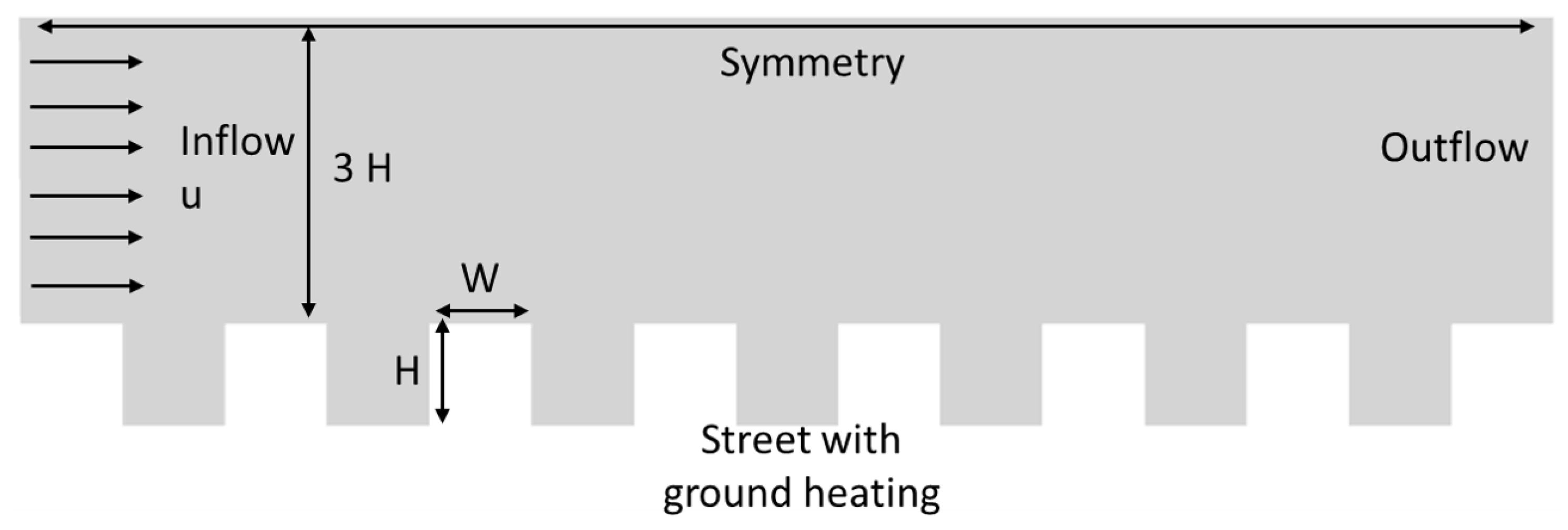
In this case study, there are seven street canyons. The building’s height, H, and width, W, are both 1 m, as illustrated in Figure 1. For the discretisation of this 2D model, a structured (trimmed cell) mesh was used. Using a 0.02 m cell size, with a stretching ratio of 1.2, approximately 420,000 rectangular elements were generated. The target street canyon with bottom heating is the middle canyon in Figure 1. Bottom heating is defined as the temperature difference between the ground’s surface and the ambient air temperature and represents the effect of the sun warming the earth. The estimated normalised potential temperature and horizontal velocity are acquired at the centerline of the target street canyon.
2.1.3. Governing Equations and Boundary Conditions
In this case study, the temperature and velocity variations are computed using coupled flow and energy equations. The flow model is based on the RANS equations with the standard k- turbulence model, as described in [28,29,30,31]. The segregated fluid temperature energy model is employed in this simulation. The energy equation is solved using the segregated fluid model in STARCCM+, with temperature as the solution variable. The equation of state is then used to calculate enthalpy from temperature [32]. The wind speed and temperature at the boundaries are given based on the bulk Richardson number (Rb), which is defined by Equation (1).
where g is the gravitational acceleration, H denotes building height, and stand for the ambient air and the ground temperature, respectively. The velocity at the building height is denoted by . The simulated case has a bulk Richardson number of −0.27 and a bottom heating of 2 °C. Wind speed at the inlet is set at 0.5 m/s. The ambient air temperature at the inlet and outlet is set at 20 °C. The outflow boundary has zero static pressure and the top of the domain is symmetric. Table 1 represents a summary of the boundary conditions for Test Case 4.
2.2. Test Cases 1 and 2: Selected Areas of East Village of London Olympic Park
2.2.1. Introduction
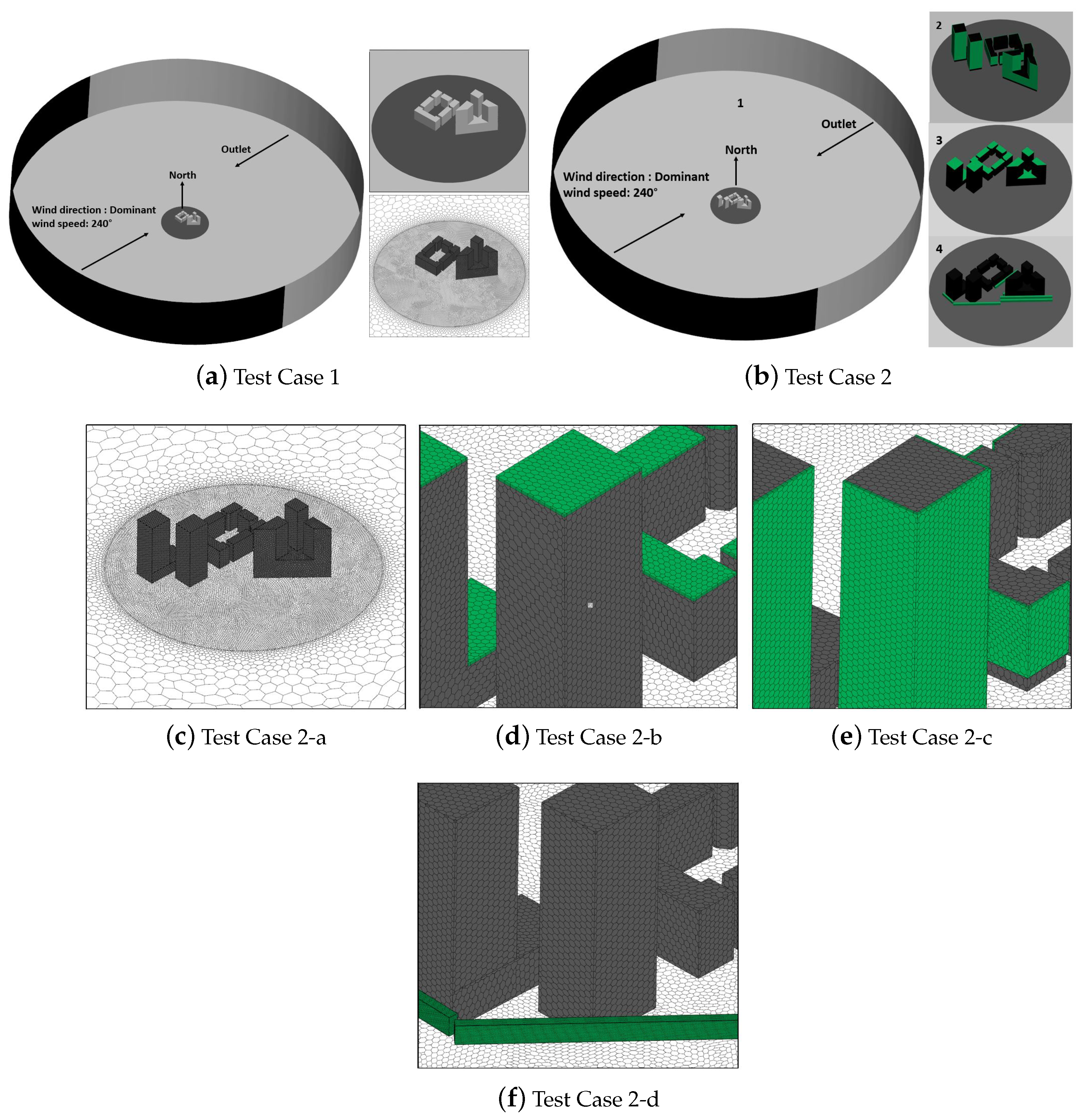
In this section, some areas of East Village are selected and presented in Figure 2a,b. Test Case 1 consists of 7 buildings, while Test Case 2 is the same as Test Case 1 but with one additional building. The focus of this section is on the impact of vegetations (trees, green roofs and green walls) on wind speed, air temperature and pollution dispersion in urban areas. The efficacy of different mitigation measures is quantified and compared in terms of the area-weighted average of temperature, pollutant concentration and velocity magnitude.
2.2.2. Computational Domain and Grid
The computational domain for all test cases in this section is the same as in [29]. Building heights for Test Case 1 range from 30 to 80 m, while those for Test Case 2 range from 30 to 102 m. In this part of East Village, the additional building in Test Case 2 is the tallest building. In Test Case 1, there is no vegetation; however, in Test Case 2, there are numerous types of vegetation that are defined in Table 2.
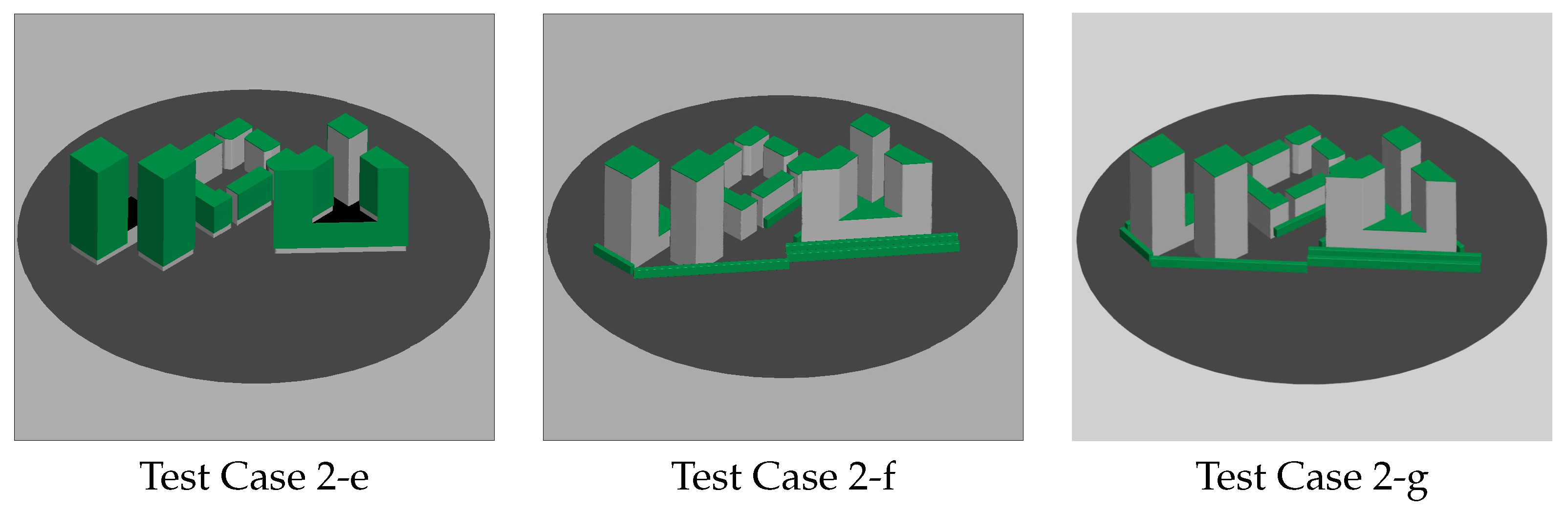
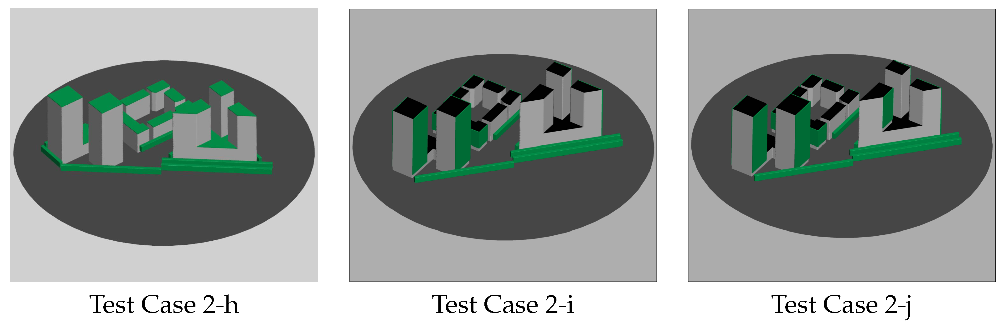
The size, type and location of trees are chosen based on the optimal layout of trees in [29]. The thickness of green walls and roofs is 1 m. Green roofs and green walls are represented in this study by a block with a thickness of 1 m, as opposed to the real case where green roofs contain numerous layers [33]. The trees are elevated 6 m above the ground, thus the green walls are similarly lifted 6 m. In Test Cases 2a and 2b, green walls and roofs are found on all of the building surfaces which are depicted by numbers 2 and 3 in Figure 2b. Apart from the influence of individual vegetation, the efficacy of combination strategies was also assessed. Figure 3, cases e–h show the combination of greenery. Cases ‘i’ and ‘j’ are targeted mitigation choices, and the reason for this configuration will be detailed in Section 3.5.
A polyhedral mesh is used for the discretisation of the domain with a thin mesh with two layers on green roofs and green walls (see Figure 2).
Figure 2.
Computational domain: (a) Test Case 1 and (b) Test Case 2. Computational mesh for Test Case 2: (c) without vegetation, (d) with green roofs, (e) with green walls and (f) with trees.
Figure 2.
Computational domain: (a) Test Case 1 and (b) Test Case 2. Computational mesh for Test Case 2: (c) without vegetation, (d) with green roofs, (e) with green walls and (f) with trees.

Figure 3.
Geometry for Test Case 2 with mitigation options.


2.2.3. Governing Equations and Boundary Conditions
The flow and energy equations included in CFD simulations of this test case are the same as those for validation case. Heat conduction is neglected, and the walls are considered thin. The simulations are all run in a steady state. The flow and surface roughness boundary conditions are the same as in Ref. [29]. For all test situations, the air temperature is set to 20 °C. Different ground temperatures were used to generate various heating intensities, which represent bottom heating and the difference between air and ground temperatures.
To evaluate the effect of vegetations (green roofs, green walls and trees) the source terms are added to the equations of momentum, turbulent kinetic energy and energy dissipation. These equations and parameters are described in depth in refs. [29,34,35,36]. The source and sink terms in the momentum, turbulent kinetic energy and turbulent dissipation energy are activated when the flow reaches the porous media zone (on trees, green walls and green roofs) according to Equations (2)–(4) (the terms in the boxes indicate the sink and source terms on trees).
where CD is the drag coefficient and ‘a’ is the leaf area density, |u| refers to the velocity magnitude and ui is the velocity component of direction i. Given that many trees in the UK are deciduous, the average value for leaf area density is fixed at 1.6. The average leaf area densities for deciduous trees are approximated between 1.06 and 2.18 m3m−3 [35]. The drag coefficients for most types of vegetation are between 0.1 and 0.3.
To account for the impact of vegetations on air temperature, a volumetric cooling power is assigned to vegetation per unit volume which is a function of the leaf area density (LAD). Based on the work of Gromke et al. [34], volumetric cooling power can be estimated as 250 W·m per LAD unity.
To model traffic emissions at the bottom of the street canyon, additional equations are required. A passive scalar model is used to model pollution. The passive scalar model, which comprises convection and diffusion terms, is chosen with an arbitrary passive scalar model to build up passive scalar tracking (here pollutant concentration). The diffusion is modelled in this study using a linear eddy-diffusivity model to calculate turbulent viscosity and the turbulent Schmidt number which are essential variables for diffusion transport. The reader is referred to [32] to learn more about passive scalar’s transport and diffusion equations.
In the simulation of contaminants in urban environments, the turbulent Schmidt number plays a key role and its effect on computed concentration was investigated in different studies [35,37,38,39]. Jiang et al. [40] investigated the effect of the Schmidt number on the projected concentration field in this study. He demonstrated that using the standard k- model, a Schmidt number of 0.4 produces the best results and that a larger value leads to an overestimation of the concentration field. Since in this study, the standard k- is chosen for the simulations and based on the references mentioned here, the value of 0.4 is specified for the turbulent Schmidt number.
The emission rate is set to 100 ppb s−1, as suggested by Baker et al. [11], and used by Moradpour et al. [41]. This number represents the average traffic volume of 930 vehicles per hour [42]. The exact location of pollution is the internal circular subdomain in Figure 2 up to a height of 1 m. Different scenarios are investigated in order to assess the impact of various types of vegetation under different conditions. These are as follows in Table 3:
3. Results and Discussion
3.1. Validation Case
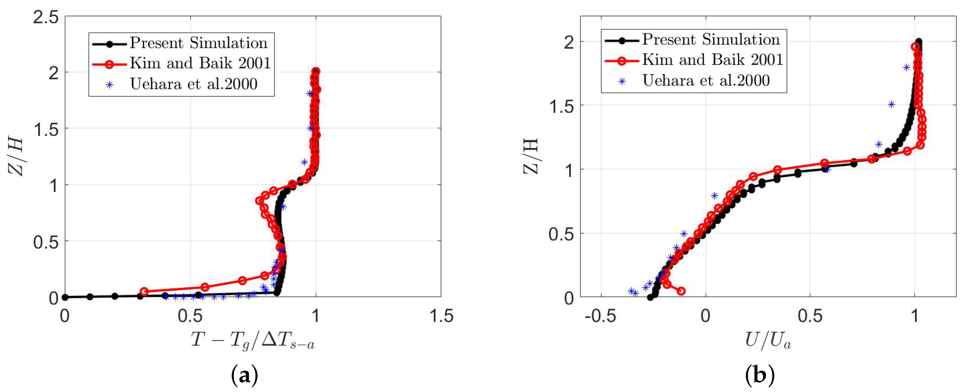
The results of this test case consist of the normalised temperature and velocity distributions in the middle of the street canyon. As shown in Figure 4, the accuracy of this model is validated by Uehara’s experimental work [23] and the study conducted by Baik et al. [25]. The estimated normalised temperature correlates well with the wind tunnel study, as shown in this figure. Furthermore, when compared to the other simulation, it is obvious that the calculated temperature near the ground is very similar to the measured data. Near the ground, the normalised velocity is overestimated while the normalised velocity derived by this model matched the wind tunnel data better than the simulation results, especially at heights beyond the roof level (Z/H > 1). Because of changes in simulated settings and experimental setup, the results of this simulation and the wind tunnel data may differ. For example, no roughness was applied to the ground when roughness elements were present in the experimental setup. Moreover, a 3D configuration was employed in the wind tunnel experiment, with buildings displayed as blocks, but the model developed in this study was 2D. Additionally, the Richardson number in the experiment is −0.21, whereas it is −0.27 in this work. Despite a few minor differences, the overall findings closely matched the wind tunnel data. Based on the results of this validation study, the same strategy for modelling energy in urban areas with bottom heating will be used for Test Cases 1 and 2.
3.2. Test Cases 1 and 2 without Vegetation
The simulation conditions for the cases in this section are based on scenario 3 in Table 3, with a bottom heating temperature of 10 °C, cooling intensity of 250 W·m−3 and an inlet wind speed of 8 m/s.
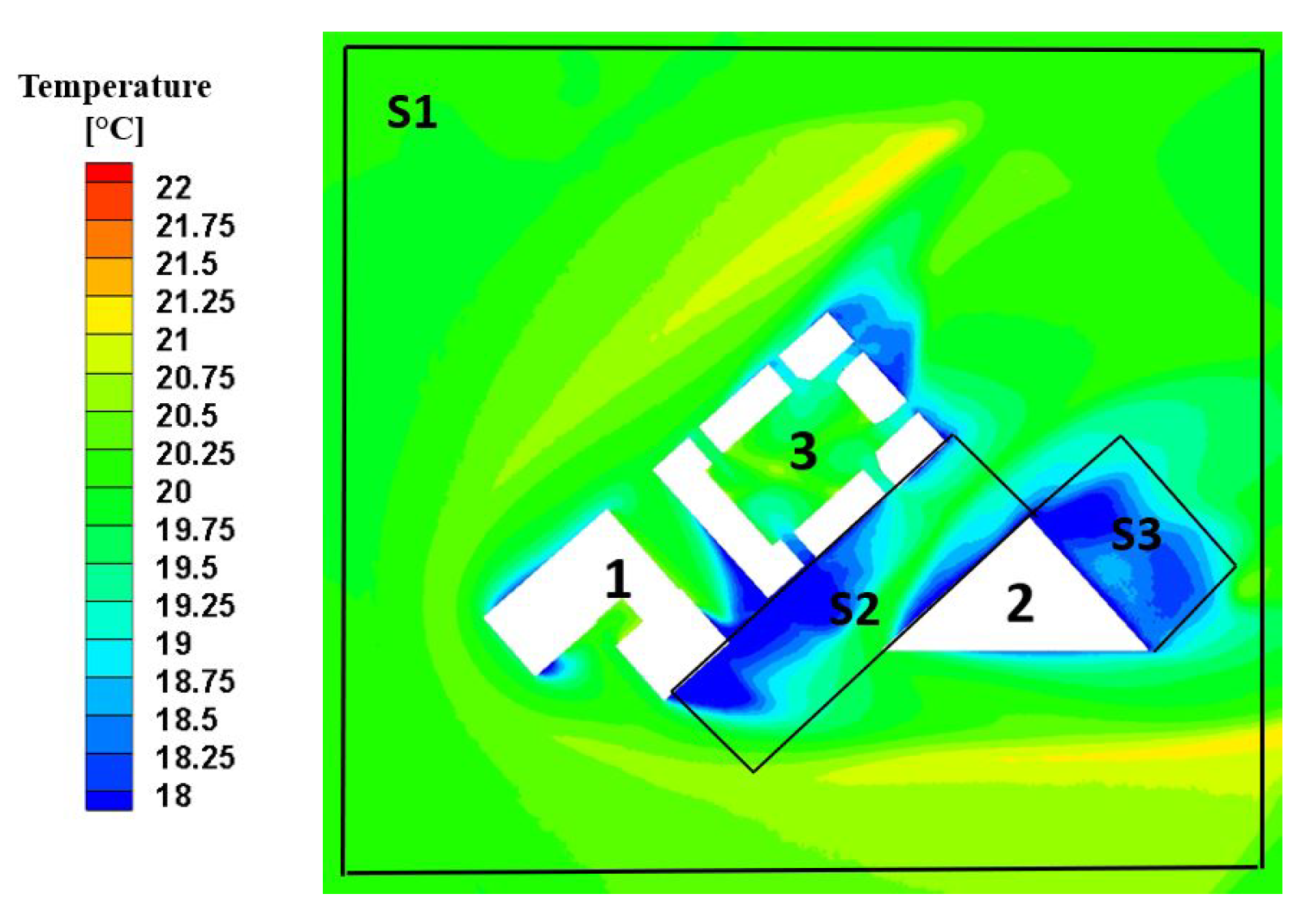
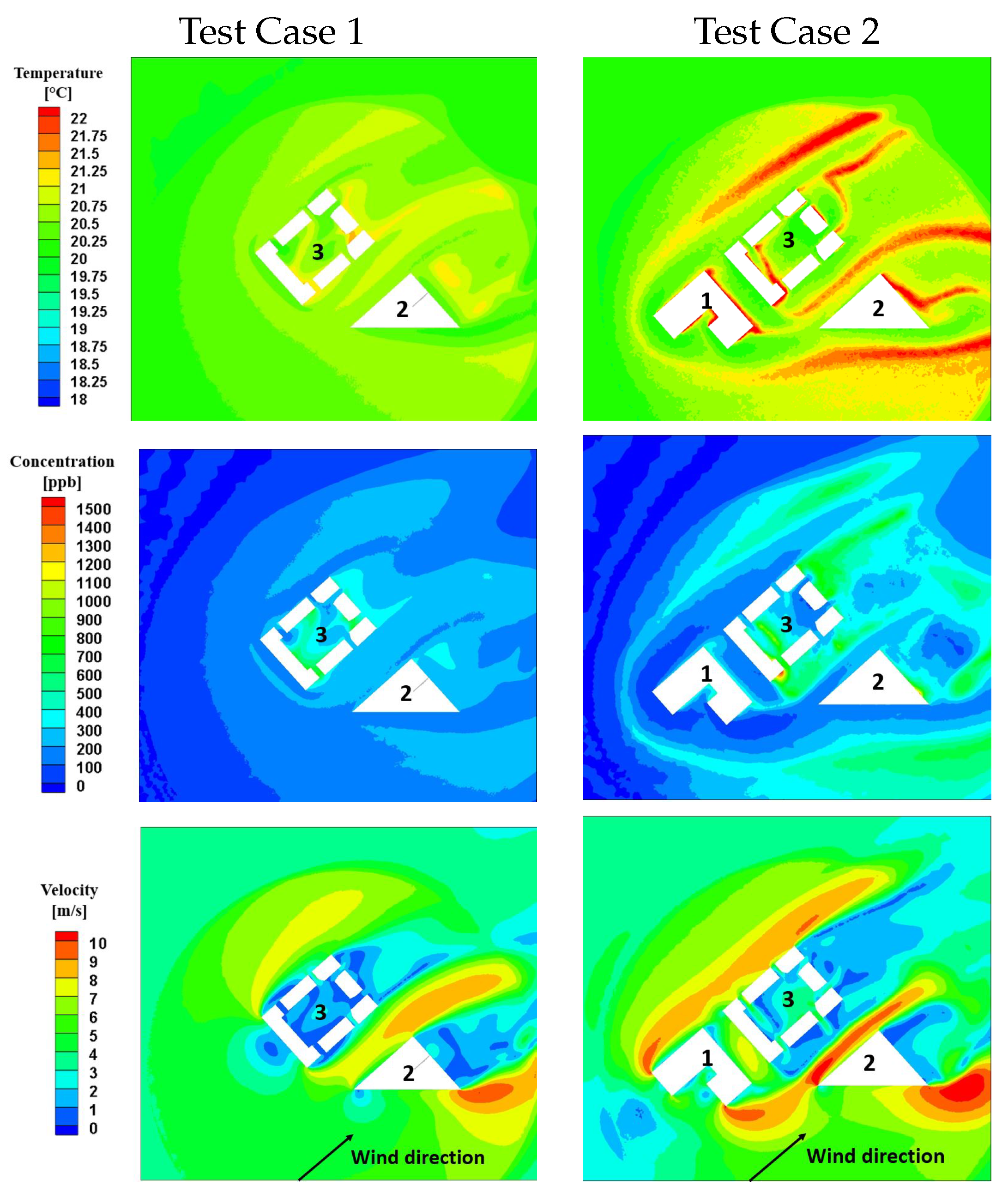
The results of this section consist of contours of temperature, pollution and velocity at the pedestrian level for Test Cases 1 and 2 as shown in Figure 6. In addition, the area-weighted average of these variables is taken in three regions of interest, S1, S2 and S3 as shown in Figure 5. S1 is the largest region, and it contains all of the buildings. S2 is the street that is surrounded by all of the buildings and S3 is behind building 2. S1, S2 and S3 have surface areas of 4.4 km2, 4500 m2 and 640 m2, respectively. Based on the results of the following sections, these regions were identified as areas of interest. By comparing the contours of the left and right sides of Figure 6, it is evident that adding a 102 m high-rise building in the direction of the wind can increase the UHI impact, degrade air quality and create pedestrian discomfort.
The results showed that adding building 1 to Test Case 1 increased the average temperature in the S1, S2 and S3 regions by 0.32 °C, 0.13 °C and 0.22 °C, respectively, while increasing the pollutant concentrations by 117, 93 and 132 ppb in the same areas. The S3 region has the lowest velocity magnitude, which is the recirculation zone, and causes the most pollution because pollutants are trapped and do not move in low-velocity areas. The average velocity in the large S1 region also increased by 6%. Although this is only a marginal increase, the addition of a building resulted in high-velocity areas in some regions due to the corner and downwash effect. When comparing Test Cases 1 and 2, it appears that the red areas which cause pedestrian discomfort have increased in size dramatically.
The quantitative comparison of these two scenarios necessitates the use of mitigation methods (e.g., vegetation) on Test Case 2 to offset the increases in temperature, pollutant concentration and velocity magnitude. In the next sections, the efficacy of different approaches under various conditions is discussed.
3.3. Test Case 2 with Mitigation Strategies
This section explores how different vegetation layouts such as green roofs, green walls, and trees affect microclimate air temperature, pollution dispersion and velocity at the pedestrian level. In order to do so, five scenarios are examined. In scenario 1, the mean flow, temperature, and pollutant characteristics are provided in the absence of bottom heating. The results of the cases with street bottom heating, referred to as scenarios 2 and 3, are then presented. The difference between scenarios 3 and 4 is that the cooling intensity in the latter is doubled. The difference between the third and fifth cases is that the velocity in the latter is half. In all cases, the average temperature, pollution and velocity magnitudes in the region of S1 are decreased by all vegetations. However, the extent of this reduction depends on street bottom heating, vegetation cooling intensity and wind speed, which are all discussed below.
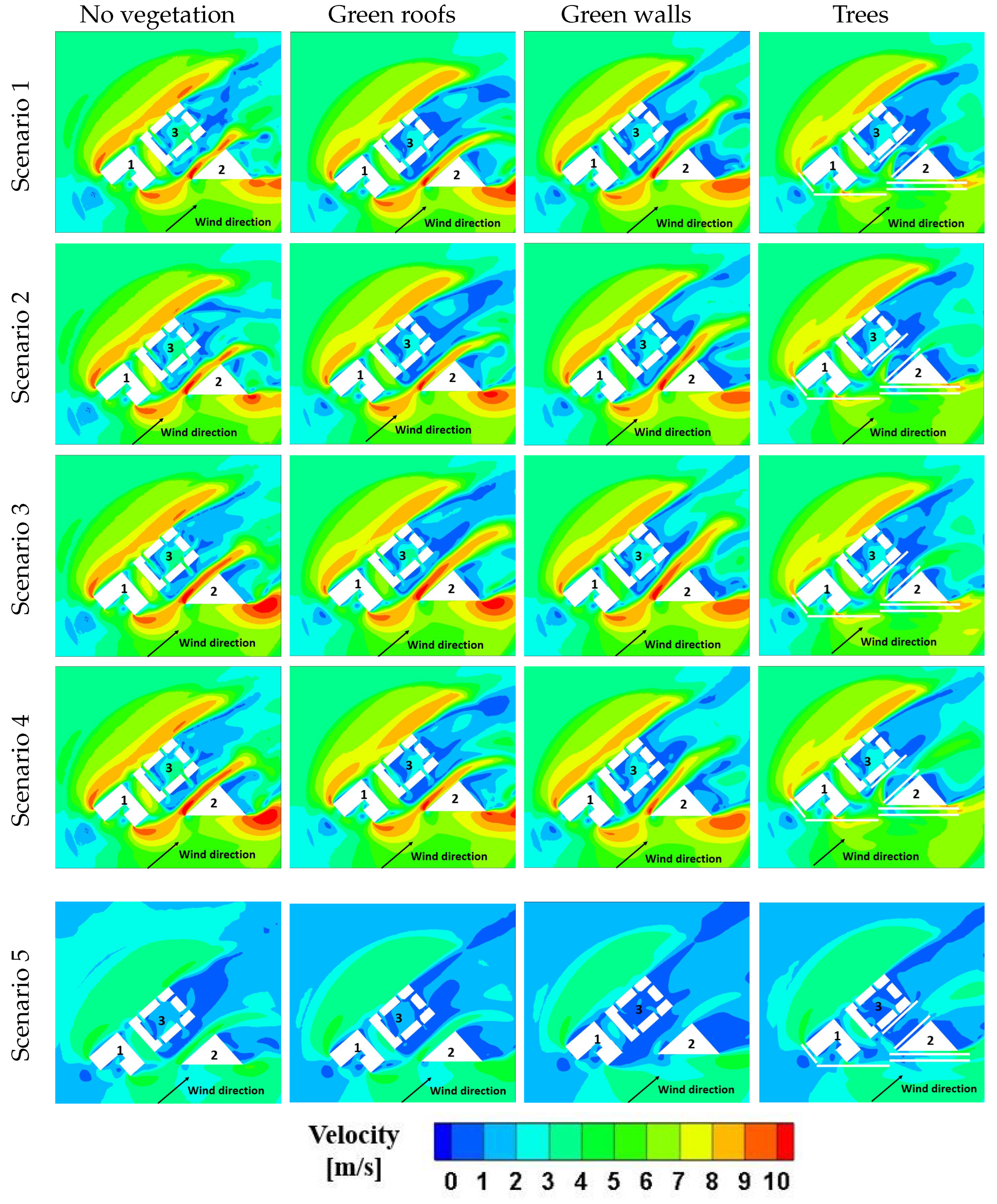
Impact of bottom heating
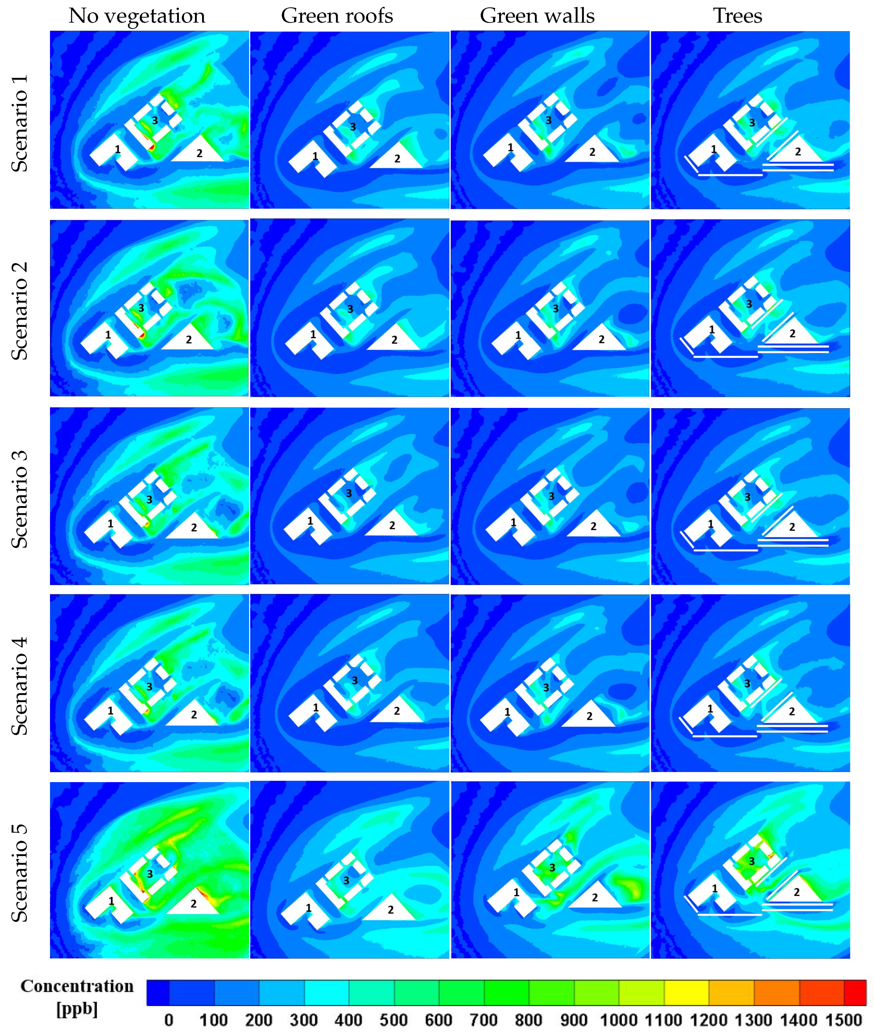
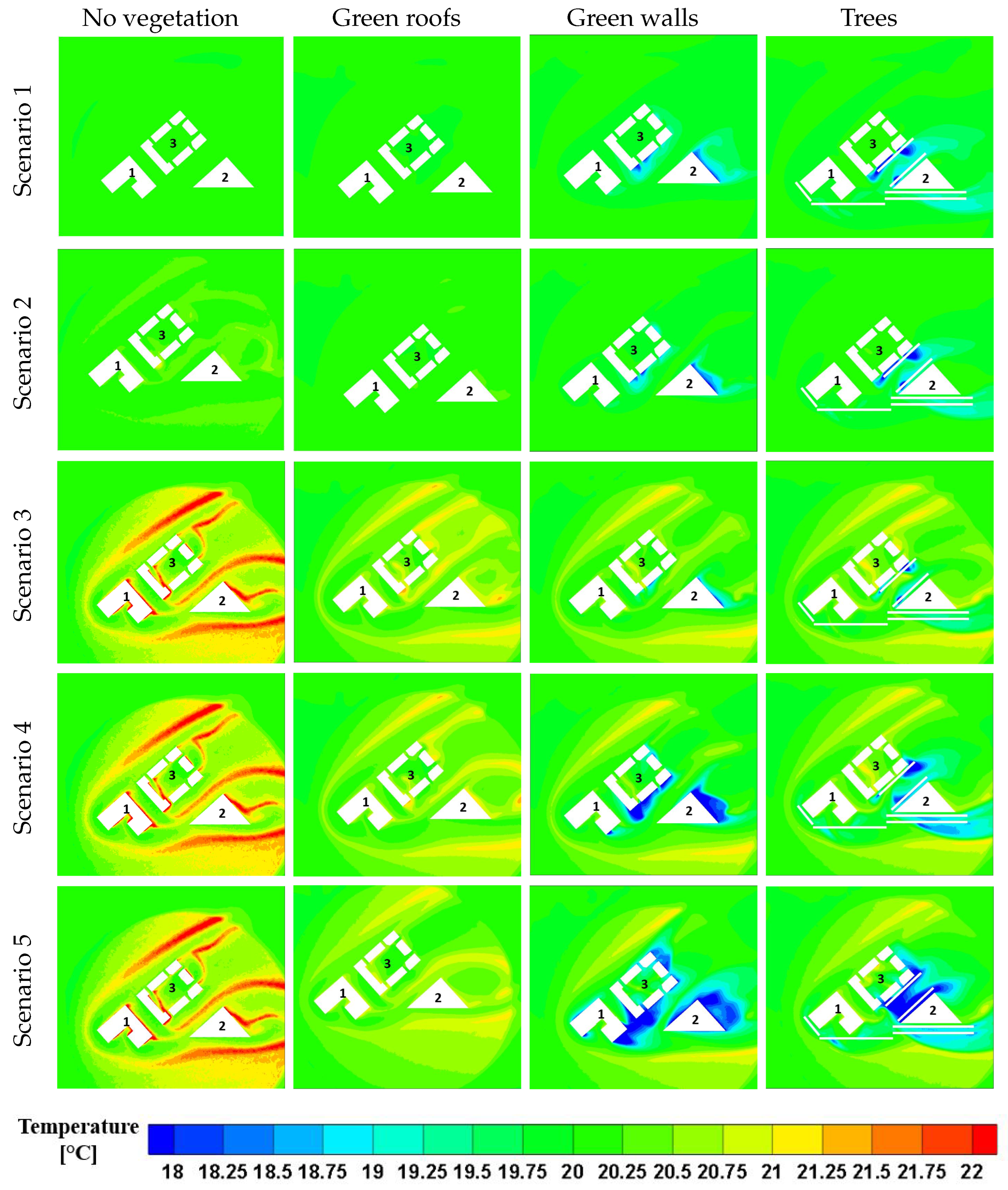
When the ground temperature rises, the average velocity magnitude at the pedestrian level goes up, especially in the S1 zone, but a comparison of Scenario 1 to 3 for the case with no vegetations in Figure 7 shows no significant variation in the mean flow pattern between cases with different bottom heating situations. The results of earlier studies [43,44] show that increasing bottom heating improves mean flow inside street canyons. According to these findings, the mean wind speed increased under unstable conditions while decreasing in calm conditions where unstable conditions correspond to bottom heating cases in this study according to the Richardson number. Under neutral conditions, trees reduce the temperature by 0.16 °C. In unstable situations, this is 0.25 °C and 0.51 °C. This means that as the bottom heating rises, vegetations become more effective at reducing temperature. Green roofs and green walls are following the same trend. A slight drop in the average pollutant concentration at the pedestrian level can be detected as the ground temperature rises [26,40,45,46]. As shown in Figure 8, pollution reduction by all vegetations in neutral and unstable situations is nearly identical.
Impact of cooling intensity of vegetation
As expected, the average air temperature drops as the cooling intensity increases and cooler air flows into the street canyon as the cooling effect becomes stronger. This can be seen by comparing scenarios 3 and 4 in Figure 9, where the only variation is the cooling intensity. Green walls and trees are the most effective solutions for lowering air temperature in the S1 zone, with a drop of 0.5 °C to 0.7 °C when cooling intensity is doubled. In scenario 3, trees reduce the temperature in region S2 by 0.95 °C, while green walls reduce the temperature by 1.43 °C in scenario 4. It is worth noting that green walls are on the façades of buildings, and trees are only found in specific regions of high velocities. In comparison to trees, increasing the cooling effects of green walls results in a greater temperature drop.
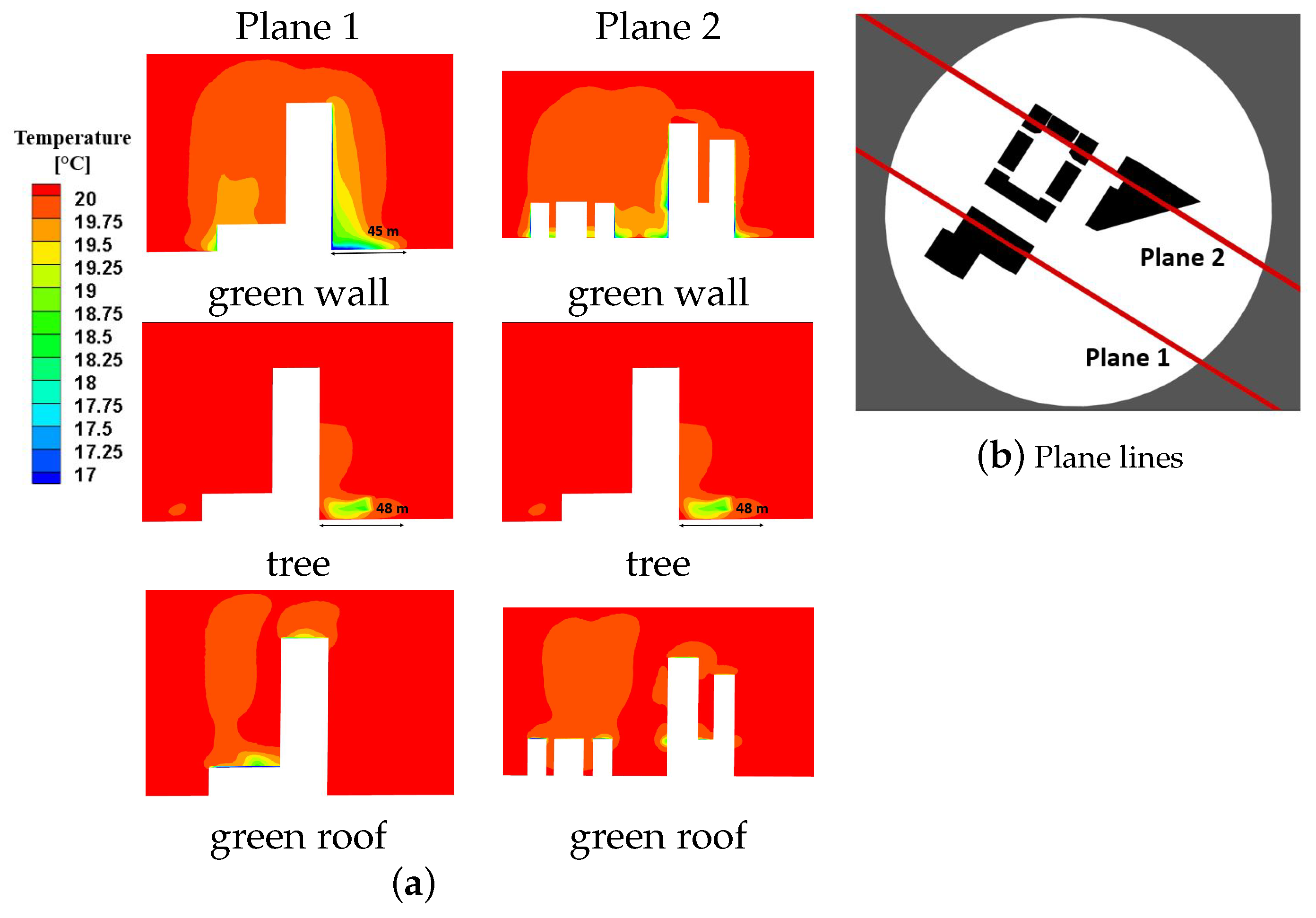
Despite the fact that the contours are given at the pedestrian level, the temperature difference is shown in two separate planes (Figure 10). This figure depicts how convection in the atmosphere distributes heat energy from warmer places near the Earth’s surface to higher altitudes in the atmosphere. This graph indicates that the comparison should not be limited to the pedestrian level. When comparing case ’a’ with case ’c’, as well as case ’d’ with case ’b’ in this figure, it can be seen that while trees are able to reduce the temperature in more areas at the pedestrian level, green walls are better in general in reducing air temperature if the vertical comparison is also made.
Impact of wind speed
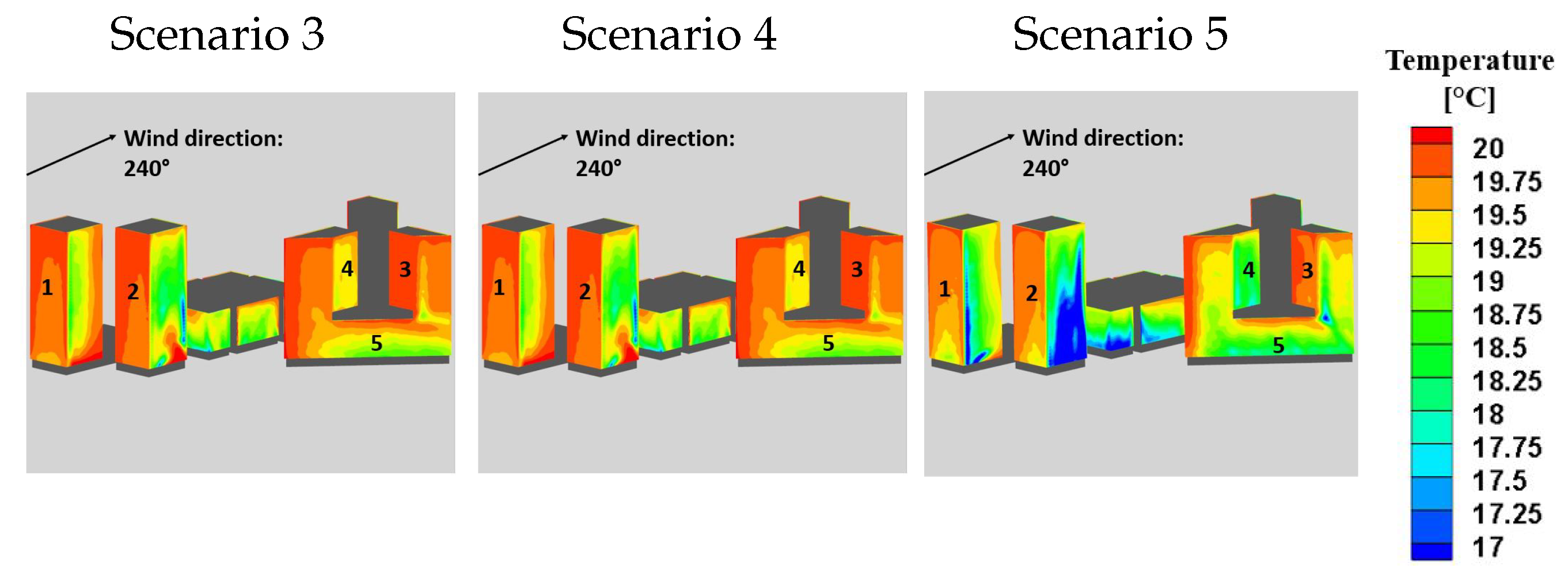
Lowering the wind speed increases the temperature gradient on vegetations, as shown in Figure 11. This observation was confirmed by the results of Fu et al. [47]. By halving the wind speed in scenario 5, the temperature reduction by green walls and trees in the S1 region is 0.9 and 0.8 °C, respectively. Because the trees are not planted at the back of buildings 2 and 3, the best comparison may be made in region S2. Furthermore, in all circumstances, lowering the wind speed at the inlet resulted in higher pollution concentrations. As a result, more windy weather leads to improved air quality [48]. According to De et al. [49], the porous nature of the vegetation can produce more mechanical turbulence and absorb more turbulent kinetic energy. Reduced wind speed and recirculation flow (wake region) result in increased shear stress and turbulence which subsequently increased the dispersion of pollutants. As a result, in the test cases studied in this section, the largest concentrations are found in the recirculation zones inside buildings 3 and in the rear of building 2.
By looking at the contours and the area-weighted average of velocity, it is clear that the trees are the best option in reducing velocity among all the tested test cases. However, trees are not as effective as green walls and green roofs in reducing pollution dispersion. In comparison to green walls and trees, the outcomes of this study demonstrate that planting green roofs on tall buildings may not be a cost-effective solution for reducing the UHI effect.
3.4. Test Case 2 with Combination of Mitigation Strategies
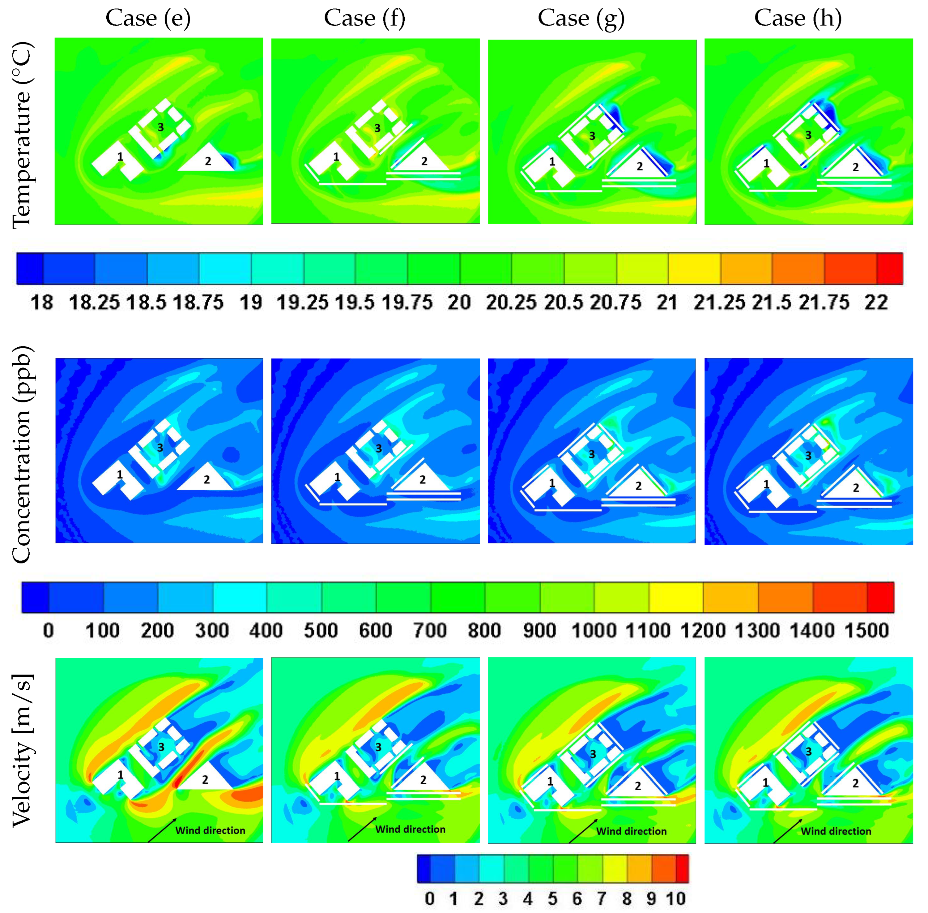
The simulation conditions for the cases in this section are based on scenario 3. In contrast to the previous section, which looked at the effectiveness of green roofs, green walls and trees individually, this section looks at how these measures perform when they are combined. The contours of temperature, pollution and velocity are presented in Figure 12. The findings of this section are compared to Test Case 2-a in scenario 3, which is a case with no vegetation.
The average temperature drop in cases ‘e’, ‘f’, ‘g’ and ‘h’ for region S1 is 0.5, 0.51, 0.67 and 0.77 °C, respectively, while pollution levels decreased by 49%, 47%, 43% and 42%, respectively. The average quantity of pollutants is reduced in the S1 region, but not in all sections of the domain, as in the other situations reviewed in the previous section. Trees are added around all buildings in cases ‘g’ and ‘h’. The back of buildings have a lower velocity and as a result, a larger level of pollution is observed than in the absence of vegetation. It can be seen that moving the tree crown 2 m closer to the ground reduced the average velocity by 2% more, while by comparing the velocity contours of cases g and h in Figure 12, it can be seen that both cases were able to reduce the uncomfortable pedestrian zone (red areas in the velocity contours) due to the corner and acceleration effect. Furthermore, when comparing examples ‘f’ and ‘g’, where the difference is the number of trees, the average velocity reduction for both cases is almost similar. The worst case scenario is combining green walls and green roofs (Case e), which failed to reduce high-velocity zones and only reduced velocity by 5% on average for the S1 region.
In comparison to the individual options (Cases a, b, c and d in Section 3.3), cases ‘g’ and ‘h’ decrease the temperature more than case ’d’ by 0.16 °C and 0.26 °C, respectively, while the pollution level increases slightly. Moreover, whether trees are used alone or in conjunction with green roofs and trees, there is no noticeable difference in the reduction of high-velocity zones. Although combining solutions can combat the UHI effect better than individual options, the economic evaluation must also take into account the operational costs, maintenance and other aspects [50].
3.5. Test Case 2 with Targeted Mitigation
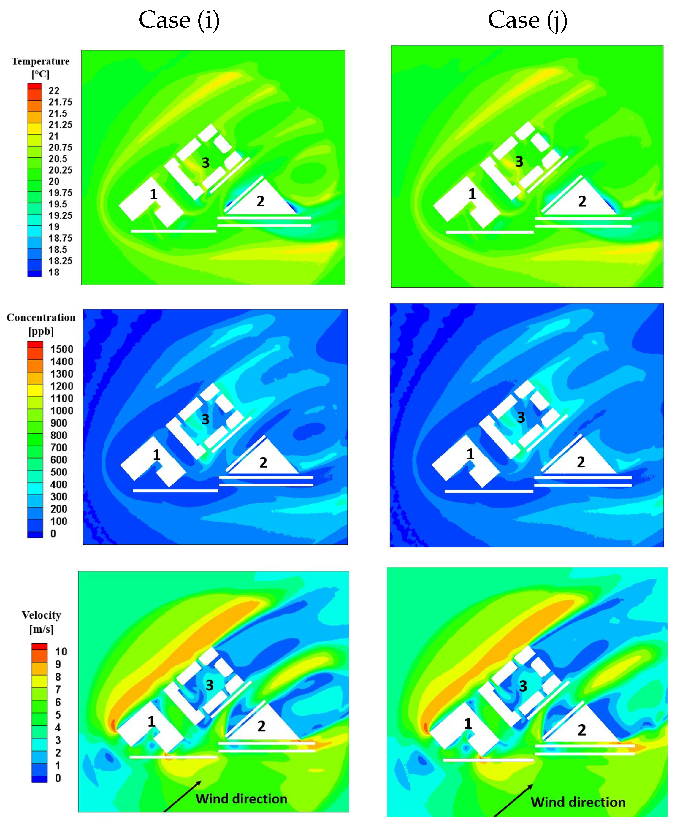
According to the results obtained in the previous section, it appears that combining green walls and trees is a viable alternative for reducing UHI, pollution and velocity. As can be observed in Figure 11, the walls facing the wind have a lower temperature gradient than the other walls in these cases. The temperature gradient on walls 1, 2 and 3 is clearly the lowest. As a result, the green walls on this surface have been removed. Although the temperature gradient on wall 5 is greater than on the other labelled surfaces, trees are chosen to be planted in front of this wall because the region in front of it is high-velocity zones (see Figure 7). Face 4 is a smaller wall with a colder surface than Faces 1, 2, and 3. So, in this part, the results of this section are compared to the Test Case 2 for scenario 3 in Figure 9. The temperature, pollutant concentration and velocity contours for cases ‘i’ and ‘j’ are presented in Figure 13. The reduction of the area-weighted average of temperature in regions S1, S2 and S3 for case ‘i’ is 0.54 °C, 0.78 °C and 0.71 °C, respectively, whereas for case ‘j’, it is 0.55 °C, 0.7 °C and 1.03 °C. When compared to Test Case 2-d (with only trees), this combination performs better in terms of temperature reduction in the S1 (largest region) and S3 regions. Trees are better in the S2 (street with buildings around it) area. For region S1, the pollution reduction is very similar to the situations with green walls, green roofs, and trees individually, but it performs better in regions S2 and S3. The average velocity reduction is also comparable to the trees. Green walls are removed from all five numbered surfaces (case ‘i’) and a scenario where green walls are removed from all numbered faces except face 4 (case ‘j’). Since there are no high-velocity areas at the back of the buildings, trees were not planted in these regions.
In comparison to the application of vegetation alone or other combination strategies, the combination of green walls and trees proved to be a better option. The ideal placement for trees to improve pedestrian comfort, as well as placing green walls on the faces that can produce the highest temperature gradient, are all factors in the optimal combination of green walls and trees. The direction and magnitude of the wind are the most important criteria in determining which walls should be green.
4. Conclusions
CFD simulations of flow, energy and pollution were performed for three test cases and the results demonstrate how including a building in an urban design can aggravate the urban heat island effect (UHI), degrade air quality and cause pedestrian discomfort. As a result, mitigation strategies (e.g., green roofs, green walls and trees) to minimise these effects must be offered. Five scenarios were tested which differ in terms of bottom heating, vegetation’s cooling intensity and the magnitude of the wind speed at the inlet. The results showed that all vegetations reduced the average temperature, pollution dispersion and velocity magnitude at the pedestrian level. In addition to evaluating vegetations individually, the effects of combining these measures were also studied. The following main conclusions can be drawn from this study.
- In comparison to green façades, trees are the most effective type of vegetation for lowering velocity due to the corner and downwash effects. Because it has a broader crown and can be planted anywhere on the street, it is the ideal option for pedestrian comfort. Green walls and roofs, on the other hand, are solely on the exteriors of buildings.
- Decreasing wind speed increases the temperature gradient on vegetation, resulting in a greater drop in air temperature at the pedestrian level. However, pollution concentration rises as wind speed decreases. The places with the highest levels of pollution are those areas with recirculation flow.
- Increasing the vegetation’s cooling intensity and leaf area density reduces the UHI effect but has little effect on changing the pattern of pollutant dispersion at the pedestrian level.
- In comparison to green walls and trees, green roofs on tall buildings are less effective at reducing temperature.
- As the ground temperature rises, a slight decrease in the average pollutant concentration at the pedestrian level can be detected. In both neutral and unstable conditions, pollution reduction by all means of vegetation is relatively similar. In addition, with increased bottom heating, vegetation is more effective at lowering the temperature.
- Overall, when considering the effects of velocity, temperature, and pollution, a combination of green walls and trees on high-speed wind and tall buildings is the best option.
It is worth noting that the results of this study can be improved in a number of ways. For instance, accurate modelling of radiation provides more realistic results. In order to provide more reliable predictions of air temperature, radiation parameters such as radiation flux, emission angle, the wavelength of radiation, surface absorptivity, reflectivity and transmissivity must be taken into account. However, bottom heating is used in this study to represent how the sun warms the earth. Moreover, the variation of the strength of bottom heating was neglected in this study and the simulations were performed with reference to a steady-state scenario. An additional limitation is that the pollutant emission considered in this study was based only on traffic data, whereas pollution can also be caused by industry. Furthermore, unlike the non-reactive pollutant suggested in this study, the pollutant in a real case study can be reactive. More accurate simulations may also require a higher level of detail in the description of the layered structure of green façades.
Author Contributions
Conceptualisation, A.H., A.B.-B. and A.K.; Software, A.H., Methodology, A.H.; Validation, A.H.; Investigation, A.H.; Visualisation, A.H.; Writing—original draft, A.H.; Resources, A.B.-B. and A.K.; Writing—review and editing, A.B.-B. and A.K. All authors have read and agreed to the published version of the manuscript.
Funding
The first author would like to acknowledge the UKRI’s funding under the ‘Exceptional Women in Engineering’ Scheme awarded by the Department of MACE at the University of Manchester.
Institutional Review Board Statement
Not applicable.
Informed Consent Statement
Not applicable.
Data Availability Statement
Data sharing is not applicable to this article.
Acknowledgments
The first author would like to acknowledge the UKRI’s funding under the ‘Exceptional Women in Engineering’ Scheme awarded by the Department of MACE at the University of Manchester.
Conflicts of Interest
The authors declare no conflict of interest.
References
- Hong, B.; Lin, B. Numerical studies of the outdoor wind environment and thermal comfort at pedestrian level in housing blocks with different building layout patterns and trees arrangement. Renew. Energy 2015, 73, 18–27. [Google Scholar] [CrossRef]
- Pierangioli, L.; Cellai, G.; Ferrise, R.; Trombi, G.; Bindi, M. Effectiveness of passive measures against climate change: Case studies in Central Italy. Build. Simul. 2017, 10, 459–479. [Google Scholar] [CrossRef]
- Oke, T.R. The energetic basis of the urban heat island. Q. J. R. Meteorol. Soc. 1982, 108, 1–24. [Google Scholar] [CrossRef]
- Mohajerani, A.; Bakaric, J.; Jeffrey-Bailey, T. The urban heat island effect, its causes, and mitigation, with reference to the thermal properties of asphalt concrete. J. Environ. Manag. 2017, 197, 522–538. [Google Scholar] [CrossRef] [PubMed]
- Grimmond, S.U. Urbanization and global environmental change: Local effects of urban warming. Geogr. J. 2007, 173, 83–88. [Google Scholar] [CrossRef]
- Mayer, H. Air pollution in cities. Atmos. Environ. 1999, 33, 4029–4037. [Google Scholar] [CrossRef]
- Fenger, J. Urban air quality. Atmos. Environ. 1999, 33, 4877–4900. [Google Scholar] [CrossRef]
- Pope, C.A., III; Ezzati, M.; Dockery, D.W. Fine-particulate air pollution and life expectancy in the United States. N. Engl. J. Med. 2009, 360, 376–386. [Google Scholar] [CrossRef] [Green Version]
- Lin, H.; Xiao, Y.; Musso, F.; Lu, Y. Green Façade Effects on Thermal Environment in Transitional Space: Field Measurement Studies and Computational Fluid Dynamics Simulations. Sustainability 2019, 11, 5691. [Google Scholar] [CrossRef] [Green Version]
- Chen, N.; Tsay, Y.; Chiu, W. Influence of vertical greening design of building opening on indoor cooling and ventilation. Int. J. Green Energy 2017, 14, 24–32. [Google Scholar] [CrossRef]
- Memon, R.A.; Leung, D.Y.; Liu, C.H. Effects of building aspect ratio and wind speed on air temperatures in urban-like street canyons. Build. Environ. 2010, 45, 176–188. [Google Scholar] [CrossRef]
- Jim, C.Y. Thermal performance of climber greenwalls: Effects of solar irradiance and orientation. Appl. Energy 2015, 154, 631–643. [Google Scholar] [CrossRef]
- Huang, J.M.; Ooka, R.; Okada, A.; Omori, T.; Huang, H. The effects of urban heat island mitigation strategies on the outdoor thermal environment in central tokyo—A numerical simulation. In Proceedings of the Seventh Asia Pacific Conference on Wind Engineering, Taipei, Taiwan, 8–12 November 2009. [Google Scholar]
- Chen, H.; Ooka, R.; Huang, H.; Tsuchiya, T. Study on mitigation measures for outdoor thermal environment on present urban blocks in Tokyo using coupled simulation. Build. Environ. 2009, 44, 2290–2299. [Google Scholar] [CrossRef]
- Liu, K.K.; Baskaran, A. Using Garden Roof Systems to Achieve Sustainable Building Envelopes; Construction Technology Update, No. 65; Institute for Research in Construction, National Research Council of Canada: Ottawa, ON, Canada, 2005. Available online: https://nrc-publications.canada.ca/eng/view/ft/?id=c95f042f-c32c-44b1-9e11-6055eadff533 (accessed on 20 November 2022).
- Hosseini, S.H.; Ghobadi, P.; Ahmadi, T.; Calautit, J.K. Numerical investigation of roof heating impacts on thermal comfort and air quality in urban canyons. Appl. Therm. Eng. 2017, 123, 310–326. [Google Scholar] [CrossRef]
- Qin, H.; Hong, B.; Jiang, R. Are green walls better options than green roofs for mitigating PM10 pollution? CFD simulations in urban street canyons. Sustainability 2018, 10, 2833. [Google Scholar] [CrossRef] [Green Version]
- Rafael, S.; Vicente, B.; Rodrigues, V.; Miranda, A.; Borrego, C.; Lopes, M. Impacts of green infrastructures on aerodynamic flow and air quality in Porto’s urban area. Atmos. Environ. 2018, 190, 317–330. [Google Scholar] [CrossRef]
- Gromke, C.; Blocken, B. Influence of avenue-trees on air quality at the urban neighborhood scale. Part II: Traffic pollutant concentrations at pedestrian level. Environ. Pollut. 2015, 196, 176–184. [Google Scholar] [CrossRef] [Green Version]
- Vranckx, S.; Vos, P. OpenFOAM CFD Simulation of Pollutant Dispersion in Street Canyons: Validation and Annual Impact of Trees. 2013. Available online: https://www.harmo.org/Conferences/Proceedings/_Varna/publishedSections/PPT/H16-088-Vranckx-p.pdf (accessed on 20 November 2022).
- Lauriks, T.; Longo, R.; Baetens, D.; Derudi, M.; Parente, A.; Bellemans, A.; Van Beeck, J.; Denys, S. Application of improved CFD modeling for prediction and mitigation of traffic-related air pollution hotspots in a realistic urban street. Atmos. Environ. 2021, 246, 118127. [Google Scholar] [CrossRef]
- Pantusheva, M.; Mitkov, R.; Hristov, P.O.; Petrova-Antonova, D. Air Pollution Dispersion Modelling in Urban Environment Using CFD: A Systematic Review. Atmosphere 2022, 13, 1640. [Google Scholar] [CrossRef]
- Uehara, K.; Murakami, S.; Oikawa, S.; Wakamatsu, S. Wind tunnel experiments on how thermal stratification affects flow in and above urban street canyons. Atmos. Environ. 2000, 34, 1553–1562. [Google Scholar] [CrossRef]
- Kim, J.J.; Baik, J.J. Urban street-canyon flows with bottom heating. Atmos. Environ. 2001, 35, 3395–3404. [Google Scholar] [CrossRef]
- Baik, J.J.; Kang, Y.S.; Kim, J.J. Modeling reactive pollutant dispersion in an urban street canyon. Atmos. Environ. 2007, 41, 934–949. [Google Scholar] [CrossRef]
- Kim, J.J.; Baik, J.J. Physical experiments to investigate the effects of street bottom heating and inflow turbulence on urban street-canyon flow. Adv. Atmos. Sci. 2005, 22, 230–237. [Google Scholar] [CrossRef]
- Xie, X.; Liu, C.H.; Leung, D.Y. Impact of building facades and ground heating on wind flow and pollutant transport in street canyons. Atmos. Environ. 2007, 41, 9030–9049. [Google Scholar] [CrossRef]
- Hosseinzadeh, A.; Keshmiri, A. The Role of Turbulence Models in Simulating Urban Microclimate. In Advances in Heat Transfer and Thermal Engineering; Springer: New York, NY, USA, 2021; pp. 675–680. [Google Scholar]
- Hosseinzadeh, A.; Keshmiri, A. Computational simulation of wind microclimate in complex urban models and mitigation using trees. Buildings 2021, 11, 112. [Google Scholar] [CrossRef]
- Dong, Z.; Gao, S.; Fryrear, D.W. Drag coefficients, roughness length and zero-plane displacement height as disturbed by artificial standing vegetation. J. Arid Environ. 2001, 49, 485–505. [Google Scholar] [CrossRef]
- Richards, P.; Hoxey, R. Appropriate boundary conditions for computational wind engineering models using the k-ε turbulence model. In Computational Wind Engineering 1; Elsevier: Amsterdam, The Netherlands, 1993; pp. 145–153. [Google Scholar]
- adapco team, C. STARCCM+-CFD Toolbox-User’s Guide. 2019. Available online: http://www.cd-adapco.com/ (accessed on 1 January 2019).
- Raji, B.; Tenpierik, M.J.; van den Dobbelsteen, A. The impact of greening systems on building energy performance: A literature review. Renew. Sustain. Energy Rev. 2015, 45, 610–623. [Google Scholar] [CrossRef] [Green Version]
- Gromke, C.; Blocken, B.; Janssen, W.; Merema, B.; van Hooff, T.; Timmermans, H. CFD analysis of transpirational cooling by vegetation: Case study for specific meteorological conditions during a heat wave in Arnhem, Netherlands. Build. Environ. 2015, 83, 11–26. [Google Scholar] [CrossRef]
- Jeanjean, A.P.; Hinchliffe, G.; McMullan, W.; Monks, P.S.; Leigh, R.J. A CFD study on the effectiveness of trees to disperse road traffic emissions at a city scale. Atmos. Environ. 2015, 120, 1–14. [Google Scholar] [CrossRef] [Green Version]
- Katul, G.G.; Mahrt, L.; Poggi, D.; Sanz, C. One-and two-equation models for canopy turbulence. Bound.-Layer Meteorol. 2004, 113, 81–109. [Google Scholar] [CrossRef]
- Gromke, C.; Buccolieri, R.; Di Sabatino, S.; Ruck, B. Dispersion study in a street canyon with tree planting by means of wind tunnel and numerical investigations–evaluation of CFD data with experimental data. Atmos. Environ. 2008, 42, 8640–8650. [Google Scholar] [CrossRef]
- Kim, J.J.; Baik, J.J. A numerical study of the effects of ambient wind direction on flow and dispersion in urban street canyons using the RNG k–ε turbulence model. Atmos. Environ. 2004, 38, 3039–3048. [Google Scholar] [CrossRef]
- Jeanjean, A.P.; Buccolieri, R.; Eddy, J.; Monks, P.S.; Leigh, R.J. Air quality affected by trees in real street canyons: The case of Marylebone neighbourhood in central London. Urban For. Urban Green. 2017, 22, 41–53. [Google Scholar] [CrossRef]
- Jiang, G.; Hu, T.; Yang, H. Effects of ground heating on ventilation and pollutant transport in three-dimensional urban street canyons with unit aspect ratio. Atmosphere 2019, 10, 286. [Google Scholar] [CrossRef] [Green Version]
- Moradpour, M.; Afshin, H.; Farhanieh, B. A numerical investigation of reactive air pollutant dispersion in urban street canyons with tree planting. Atmos. Pollut. Res. 2017, 8, 253–266. [Google Scholar] [CrossRef]
- Mattai, J.; Hutchinson, D.; Authority, G.L. London Atmospheric Emissions Inventory. 2000. Available online: https://www.umad.de/infos/cleanair13/pdf/full_388.pdf (accessed on 20 November 2022).
- Li, X.X.; Britter, R.E.; Koh, T.Y.; Norford, L.K.; Liu, C.H.; Entekhabi, D.; Leung, D.Y. Large-eddy simulation of flow and pollutant transport in urban street canyons with ground heating. Bound.-Layer Meteorol. 2010, 137, 187–204. [Google Scholar] [CrossRef] [Green Version]
- Cheng, W.; Liu, C.H. Large-eddy simulation of turbulent transports in urban street canyons in different thermal stabilities. J. Wind. Eng. Ind. Aerodyn. 2011, 99, 434–442. [Google Scholar] [CrossRef] [Green Version]
- Baik, J.J.; Kim, J.J. A numerical study of flow and pollutant dispersion characteristics in urban street canyons. J. Appl. Meteorol. 1999, 38, 1576–1589. [Google Scholar] [CrossRef]
- Kim, J.J.; Baik, J.J. A numerical study of thermal effects on flow and pollutant dispersion in urban street canyons. J. Appl. Meteorol. 1999, 38, 1249–1261. [Google Scholar] [CrossRef]
- Fu, J.; Zhang, T.; Li, M.; Li, S.; Zhong, X.; Liu, X. Study on flow and heat transfer characteristics of porous media in engine particulate filters based on lattice Boltzmann method. Energies 2019, 12, 3319. [Google Scholar] [CrossRef]
- Cichowicz, R.; Wielgosiński, G.; Fetter, W. Effect of wind speed on the level of particulate matter PM10 concentration in atmospheric air during winter season in vicinity of large combustion plant. J. Atmos. Chem. 2020, 77, 35–48. [Google Scholar] [CrossRef]
- De Maerschalck, B.; Maiheu, B.; Janssen, S.; Vankerkom, J. CFD-modelling of complex plant-atmosphere interactions: Direct and indirect effects on local turbulence. In Proceedings of the CLIMAQS Workshop ‘Local Air Quality and its Interactions with Vegetation’, Antwerp, Belgium, 21–22 January 2010; pp. 21–22. [Google Scholar]
- Manso, M.; Teotónio, I.; Silva, C.M.; Cruz, C.O. Green roof and green wall benefits and costs: A review of the quantitative evidence. Renew. Sustain. Energy Rev. 2021, 135, 110111. [Google Scholar] [CrossRef]
Figure 1.
Seven street canyons with bottom heating in the middle street.

Figure 4.
Variation of normalised velocity and temperature with the height in the middle of target street canyon with bottom heating (a) normalised temperature; (b) normalised velocity [23,25].

Figure 5.
Regions S1, S2 and S3: Area-weighted average for temperature, concentration and velocity.

Figure 6.
Comparison of temperature, velocity and pollution contours for Test Cases 1 and 2 at the pedestrian level (2 m), bottom heating: 10 °C, cooling intensity: 250 W·m−3 and wind speed at the inlet: 8 m/s.
Figure 6.
Comparison of temperature, velocity and pollution contours for Test Cases 1 and 2 at the pedestrian level (2 m), bottom heating: 10 °C, cooling intensity: 250 W·m−3 and wind speed at the inlet: 8 m/s.

Figure 7.
Contours of velocity at the pedestrian level.

Figure 8.
Contours of pollutant concentration at the pedestrian level.

Figure 9.
Contours of temperature at the pedestrian level.

Figure 10.
(a) Contours of temperature at different planes for scenario 4 using green walls, trees and green roofs; (b) Location of planes.
Figure 10.
(a) Contours of temperature at different planes for scenario 4 using green walls, trees and green roofs; (b) Location of planes.

Figure 11.
Contours of temperature at the surface of green walls.

Figure 12.
Contours of temperature, pollutant concentration and velocity at the pedestrian level for scenario 3 with a combination of: (e) green roofs and green walls; (f) green roofs and trees; (g) green roofs and more trees; (h) green roofs and trees with trees 2 m closer to the ground.
Figure 12.
Contours of temperature, pollutant concentration and velocity at the pedestrian level for scenario 3 with a combination of: (e) green roofs and green walls; (f) green roofs and trees; (g) green roofs and more trees; (h) green roofs and trees with trees 2 m closer to the ground.

Figure 13.
Contours of temperature, pollution and velocity at the pedestrian level (2 m), bottom heating: 10 °C, cooling intensity: 250 W·m−3, wind speed at the inlet: 8 m/s. (i) first targeted combination of green walls and tree; (j) second targeted combination of green walls and tree.
Figure 13.
Contours of temperature, pollution and velocity at the pedestrian level (2 m), bottom heating: 10 °C, cooling intensity: 250 W·m−3, wind speed at the inlet: 8 m/s. (i) first targeted combination of green walls and tree; (j) second targeted combination of green walls and tree.


Table 1.
Boundary conditions for validation case.
| Boundary Conditions | Value/Definition |
|---|---|
| Inflow wind speed (m/s) | 0.5 |
| Width of street canyons (m) | 1 |
| Height of buildings (m) | 1 |
| Air temperature (°C) | 20 |
| Ground temperature (°C) | 22 |
| Richardson number | −0.27 |
| Outflow | Zero static pressure |
| Top of the domain | Symmetry |
Table 2.
Test Case 2 with various forms of vegetation.
| Case Number | Description |
|---|---|
| Test Case 2-a | Without vegetation |
| Test Case 2-b | With green roofs |
| Test Case 2-c | With green walls |
| Test Case 2-d | With trees |
| Test Case 2-e | With a combination of green roofs and green wall |
| Test Case 2-f | With a combination of green roofs and trees |
| Test Case 2-g | With a combination of green roofs and more trees |
| Test Case 2-h | With a combination of green roofs and more trees: trees 2 m closer to the ground |
| Test Case 2-i | With a targeted combination of green walls and trees |
| Test Case 2-j | With a targeted combination of green walls and trees |
Table 3.
Different scenarios for Test Case 2.
| Bottom Heating (°C) | Cooling Intensity (W·m−3) | Wind Speed at the Height of 10 m: (m/s) | |
|---|---|---|---|
| Scenario 1 | 0 | 250 | 8 |
| Scenario 2 | 2 | 250 | 8 |
| Scenario 3 | 10 | 250 | 8 |
| Scenario 4 | 10 | 500 | 8 |
| Scenario 5 | 10 | 250 | 4 |
Publisher’s Note: MDPI stays neutral with regard to jurisdictional claims in published maps and institutional affiliations. |
© 2022 by the authors. Licensee MDPI, Basel, Switzerland. This article is an open access article distributed under the terms and conditions of the Creative Commons Attribution (CC BY) license (https://creativecommons.org/licenses/by/4.0/).
Share and Cite
MDPI and ACS Style
Hosseinzadeh, A.; Bottacin-Busolin, A.; Keshmiri, A. A Parametric Study on the Effects of Green Roofs, Green Walls and Trees on Air Quality, Temperature and Velocity. Buildings 2022, 12, 2159. https://doi.org/10.3390/buildings12122159
AMA Style
Hosseinzadeh A, Bottacin-Busolin A, Keshmiri A. A Parametric Study on the Effects of Green Roofs, Green Walls and Trees on Air Quality, Temperature and Velocity. Buildings. 2022; 12(12):2159. https://doi.org/10.3390/buildings12122159
Chicago/Turabian StyleHosseinzadeh, Azin, Andrea Bottacin-Busolin, and Amir Keshmiri. 2022. "A Parametric Study on the Effects of Green Roofs, Green Walls and Trees on Air Quality, Temperature and Velocity" Buildings 12, no. 12: 2159. https://doi.org/10.3390/buildings12122159
Note that from the first issue of 2016, this journal uses article numbers instead of page numbers. See further details here.