
The Battery Life Estimation of a Battery under Different Stress Conditions


C.R. ENEA Casaccia, Via Anguillarese 301, 00123 Rome, Italy
*
Author to whom correspondence should be addressed.
Batteries 2021, 7(4), 88; https://doi.org/10.3390/batteries7040088
Submission received: 29 September 2021
/
Revised: 27 October 2021
/
Accepted: 14 December 2021
/
Published: 18 December 2021
(This article belongs to the Special Issue Lithium-Ion Batteries Aging Mechanisms, 2nd Edition)
Abstract
:The prediction of capacity degradation, and more generally of the behaviors related to battery aging, is useful in the design and use phases of a battery to help improve the efficiency and reliability of energy systems. In this paper, a stochastic model for the prediction of battery cell degradation is presented. The proposed model takes its cue from an approach based on Markov chains, although it is not comparable to a Markov process, as the transition probabilities vary with the number of cycles that the cell has performed. The proposed model can reproduce the abrupt decrease in the capacity that occurs near the end of life condition (80% of the nominal value of the capacity) for the cells analyzed. Furthermore, we illustrate the ability of this model to predict the capacity trend for a lithium-ion cell with nickel manganese cobalt (NMC) at the cathode and graphite at the anode, subjected to a life cycle in which there are different aging factors, using the results obtained for cells subjected to single aging factors.
1. Introduction
Over the past two decades, batteries have become an important part of our lifestyle: from portable electronics to electric vehicles, to the recent integration of renewable energy into the power grid. In addition to the results obtained with the aim of increasing energy and power density, much effort has been made to understand the intrinsic degradation processes that occur during the service life, leading to a continuous deterioration of the health of the cell battery, such as a loss of capacity or increase in internal resistance. Understanding the impact of the aging factors is also essential for developing reliable diagnostic and prognostic tools. However, predicting the battery aging trajectory is technically difficult because battery degradation is a complex non-linear process with coupled physical and chemical reactions, and battery life is highly dependent on applications (cycle life) or storage conditions (calendar life) [1]. One of the simplest solutions to obtain the battery capacity degradation trajectory is to conduct direct experiments in a specific load or storage condition. However, this solution generally requires a rather long experimental time of several months or even years. On the other hand, the accelerated tests must be appropriately designed to extrapolate the aging of cells under normal conditions, according to non-trivial protocols [2].
Battery degradation is affected by many factors, both at the individual cell level and the assembly level, and their effects are often correlated [3]. As the system is assembled, starting from single cells to modules and battery packs, the possible causes of stress for the batteries increase and their coupling intensifies [4]. It is therefore essential to understand the phenomenon of aging as early as possible in the complexity chain [5,6].
At the single-cell level, the degradation factors have thermodynamic and kinetic origins. Changes in the initial cell properties are influenced by the environment (e.g., temperature or pressure) and the duty cycle (e.g., voltage and current intensity) [7,8]. Batteries deteriorate even when not in use (so-called “calendar life”) and storage conditions, mainly the temperature and state of charge (SOC), affect the rate of degradation and battery performance [9].
Cycle aging refers to aging due to the continuous charge/discharge cycle of the battery. Calendar aging inevitably occurs during the life of the battery, regardless of the operating mode, and all factors of calendar aging also affect cyclic aging, especially when the battery duty cycle is made up of work phases alternating with rest phases [10]. Cycle life, however, is influenced by additional factors, such as the intensity of the current and the depth of discharge of the cycles. These aging factors act in such a way that the effects are not linearly correlated, which greatly complicates the understanding and description of the aging process. In particular, the temperature represents a very relevant factor in the degradation of the batteries, both in the operating conditions defined by the battery manufacturer, [11,12] and in the case of uncontrolled temperature conditions [12]. Since this aging factor has been extensively covered in the literature, in the present work, the temperature remains constant during the life tests, to emphasize the effects of the other stress factors.
The article is structured as follows: Section 2 illustrates the main battery degradation mechanisms and the most popular modeling approaches. Section 3 describes the setup of the experimental tests and introduces the model proposed for the degradation of battery capacity. Finally, the main conclusions are summarized in Section 4.
2. Battery Aging and Modeling
There are different mechanisms of aging and to facilitate their understanding and interpretation, they are commonly grouped into three different modes of degradation:
- Loss of conductivity (CL);
- Loss of active material (LAM), due to the degradation processes in which the use of the active electrode material is reduced;
- Loss of the lithium supply (LLI), caused by side reactions that irreversibly consume a portion of the lithium available in the cell.
The CL includes the degradation of the electronic parts of the battery, such as the corrosion of the current collector or decomposition of the binder. The LAM is related to the structural transformations of the active material and the decomposition of electrolytes, such as the oxidation of the electrolyte, the intercalation gradient in the active particles, and the disturbance of the crystal structure. The LLI is attributed to the change in the number of lithium ions available for the electrochemical cell intercalation and de-intercalation processes, electrolyte decomposition, lithium plating, and lithium-ion granule formation. Some degradation mechanisms are caused by the mechanical action of the displacement, intercalation, and de-intercalation of the ions: in electrode-active materials, the insertion/extraction of lithium ions is, in general, accompanied by the local deformation and volume variation of the materials. Due to the inherent non-equilibrium working conditions of the cells, this deformation is inhomogeneous in the materials and causes high internal stress, which ultimately leads to fracture, fragmentation, or pulverization. Due to a loss of contact with the conductive agents or electrolytes, the active materials can become partially inactive, thus contributing to the loss of the overall capacity and loss of power and promoting fracture or delamination at the interface [1,7,8]. All battery components are affected by the degradation phenomena. At the graphite anode, the intercalation of the solvent, the peeling of graphite, and the cracking due to intercalation cause LAM and LLI, and are usually accelerated with overcharging. The dissolution of the electrolyte and binder results in a loss of capacity and power capability, while the continuous growth of SEI results in an increase in the impedance [13]. These degradation mechanisms are absent if lithium titanate oxide (LTO) is used as an anode and if there is gassing due to the parasitic reactions of the LTO with the electrolyte at high temperatures, with SOC being mainly responsible for the aging [14].
The degradation process at the cathode depends on its composition. In general, the structural disordering, migration of soluble species, electrolyte decomposition, and corrosion of conductors are the main degradation phenomena. The doping of cathode with suitable materials can counteract the aging effects. For lithium-rich manganese-based layered oxides, doping leads to an increased reversible capacity, with an improved rate capability [15].
The degradation can be measured through the progressive loss of capacity (which results in a decrease in autonomy) and the increase in internal resistance, which leads to a decrease in the power delivered. The fact that the performance losses are progressive poses the problem of the definition of end of life (EOL) for Li-ion batteries. In the present work, the EOL condition is set at 20% reduction of the initial capacity following the ISO 12405-2 standard: “Electrically propelled road vehicles—Test specification for lithium-ion traction battery packs and systems—Part 2: High-energy applications” [16].
Battery cell-level aging analysis is one of the key aspects for the successful and reliable design of large-format energy storage systems based on lithium-ion technology. Ideally, the aging model should be valid for any real condition. The model must be developed based on the analysis of the different causes that affect aging, i.e., stress or impact factors, such as SOC, temperature, DOD, current rate (C-rate), and ampere-hour throughput (AhThroughput), or the number of cycles, appropriately defined.
To obtain effective battery aging predictions that can be used also for online prediction applications, the starting point is thus the experimental degradation trajectories, to which various methods can be applied to extract the battery degradation tendency over time, so that future predictions can be made with a reasonable degree of confidence. There are many algorithms for these predictions, such as those based on artificial intelligence or on filters, which are very useful in online forecasts [17].
An effective type of approach is represented by the class of models based on the physics and chemistry of the storage systems, the so-called electrochemical models. They make use of different partial differential equations systems to model the physicochemical phenomena that occur in the battery and directly explain the aging behavior of the same. In most cases, they refer to the works of Doyle, Fuller, and Newman [18,19,20], in which charge and discharge phenomena are modeled [21] along with the relaxation phenomena of lithium insertion processes [22], making use of the theory of concentrated solutions. These models are usually very accurate, but they are also generally very computationally expensive [23].
Analytical approaches are also quite widespread. Equivalent circuit models are among the most popular, since they have a level of accuracy that can be satisfactory, a lower complexity than electrochemical models and much shorter simulation times.
The simplest equivalent circuit is an ideal voltage source and resistance. However, the accuracy of this model is very low. If a capacity–resistance (RC) system is added, the model can reproduce the battery polarization effects, becoming more reliable. These types of equivalent circuits are called “Thevenin models”. Adding further RC networks to the equivalent circuit, the models become more adherent to reality, but the complexity of the resolution increases [21].
Alternatively, empirical models, such as the single exponential model, the double exponential model, the linear model, or the polynomial model, are often adopted [24]. Common to these empirical models is an explicit mathematical form and ease of implementation; however, these models tend to be sensitive to noise, especially when training data are limited.
Statistical approaches rely heavily on experimental data to predict battery behavior. Stochastic models describe the battery in an abstract way, as in analytical models. An example of a statistical approach is the autoregressive moving average (ARMA), which uses time series to deduce the aging level [25]. Particle filtering is another possible statistical approach that can predict the trend of the battery degradation [26].
The Bayesian approach to failure theory can also be applied to the EOL estimation, and the Weibull law is among the most used formula [27]. The Markov chains can also be used to describe the aging phenomenon; in particular, they can reproduce charge recovery and capacity recovery (an effect that implies a partial recovery of the battery capacity and that can occur during a period of inactivity in the charge and discharge phase) and Peukert’s law [28].
In the present work, we have considered a model inspired by the theory of Markov chains and, based on the collected data, we have verified its prediction accuracy for NMC-graphite lithium-ion cells.
3. Experimental Set Up and Modeling
In this Section, we illustrate the principal characteristics of the experimental set up and the tests conducted, and introduce the model used to interpret the data.
3.1. Life Tests for Lithium-Ion Cells
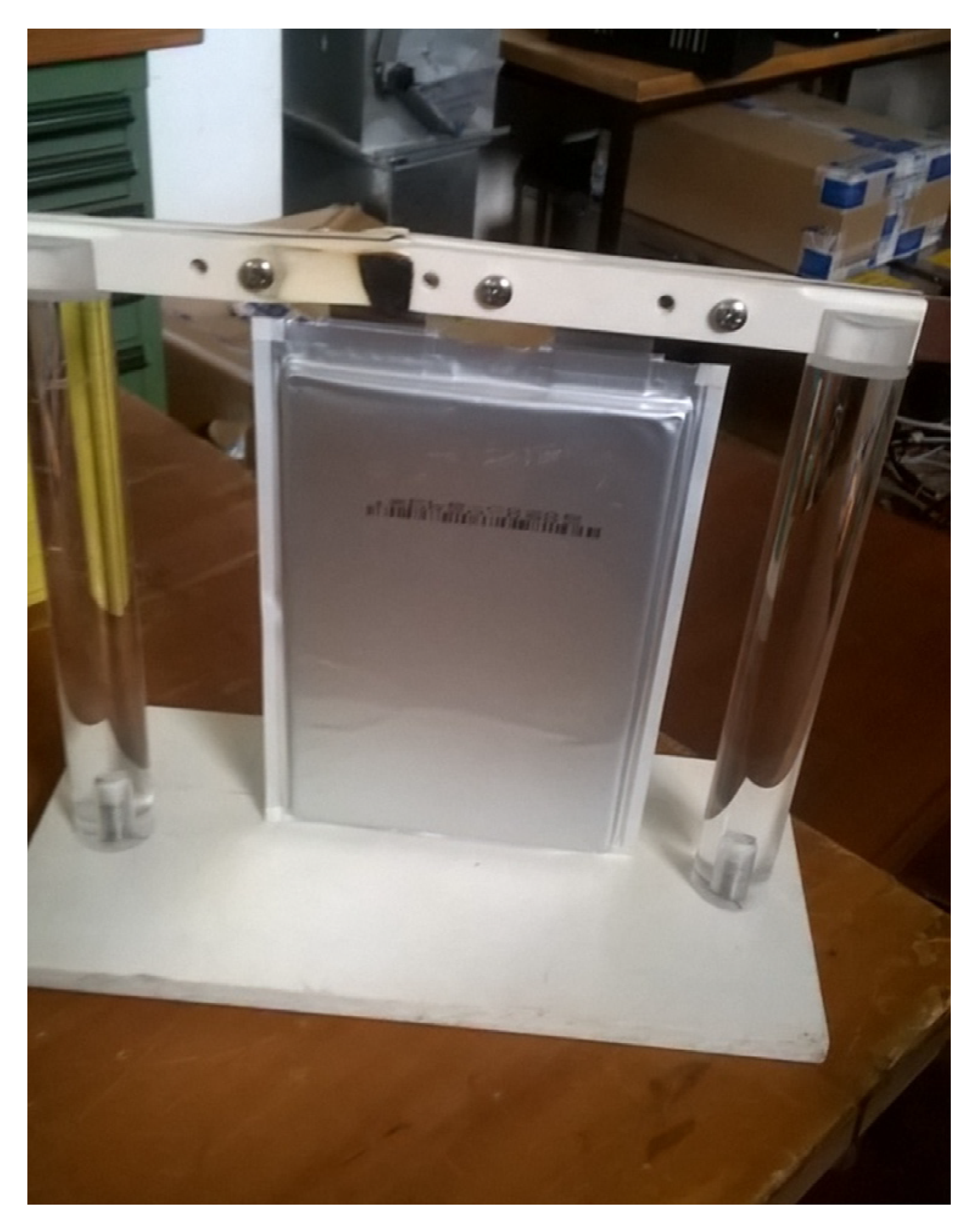
The purpose of the tests is to investigate the effect of some external factors on battery life. In particular, life tests were performed by varying the intensity of the discharge current and the depth of discharge. There are many parameters that influence the life duration of a cell, including charge current and temperature. However, finite time and equipment resources limited the number of stresses analyzed. Since we focus on stationary applications, charge current and temperature are the same in all the tests. The tests are performed on EiG PLB C020 20 Ah cells, which are lithium-ion-polymer batteries with a cathode NMC technology, graphite at the anode, and a pouch structure (see Figure 1).
The ENEA battery measurements campaign was launched in 2015, and the equipment used and the experimental protocols proposed are briefly described below.
The main electrical and operating characteristics of the cells are shown in Table 1. The life cycle of these cells is declared as 1000 cycles at 25 °C, with a depth of discharge (DoD) of 100%, and a current rate for charge and discharge of 1 C. The condition for the end of life (EOL) corresponds to a 20% decrease in the capacity to the nominal value. All the parameters of our tests fall within the limits indicated by the manufacturer in the datasheet.
The equipment used for the life tests is summarized in Table 2. In particular, the table summarizes the main characteristics and the operating range of the bidirectional AC/DC converters (cyclers) used both in the cell formation phase and for the execution of life tests and tests of the capacity and internal resistance, and of the climatic chambers in which the life tests and tests were conducted.
For each cell subjected to the test, the following steps were carried out:
- (1)
- Initial inspection, to verify the absence of damage to the cell visible from the outside and the correspondence of the physical characteristics with those provided by the manufacturer. In our case, none of the tested cells were found to have any damage or discrepancies from the physical characteristics provided in the datasheet.
- (2)
- Electrical formation: consisting of a sequence of standard cycles (discharge at constant current (CC) at C/2, pause 1 h, charge at constant current-constant voltage (CC-CV) with current at C/2, and pause 1 h), which ends when the discharge capacity relating to 2 consecutive discharges does not vary more than 3% of the value of the nominal capacity. The procedure ensures that the cells have reached an adequate stabilization of performance, before starting the actual test sequence.
- (3)
- Life cycles and periodic tests (see Section 3.1.1).
- (4)
- Final inspection, to verify the presence of any damage and deformations that occurred during the tests.
3.1.1. Life Test Procedures
During the tests, various parameters are measured and recorded, among which are: date and time, battery voltage, current, capacity and energy, and environment and battery temperature. The parameters are measured and recorded with a sufficiently high frequency to capture all the relevant variations and make them available for further data processing. Depending on the technology of the cycler used, the detection takes place at a frequency established for each phase and/or when the variation of some parameters is higher than a certain limit.
Before each test, the cells are thermally stabilized through the use of a climatic chamber. To ensure that the initial conditions of the tests are always the same, at the beginning of each test a standard cycle is performed at the same temperature at which the life tests are performed (T = 35 °C).
After the standard cycle, life tests are performed to highlight the link between the various cycling parameters studied and the decay curve of the performance of the cells being analyzed. The tests are periodically interrupted to carry out pre-established checks on the capacity and internal resistance.
The main parameters of the life tests are reported in Table 3. The cycles are balanced concerning the amount of charge delivered/accumulated. The average state of charge (SOC) of the battery is fixed at SOCav = 50% and the charging current at 0.5 C.
In tests from 1 to 4, the stress for different discharge currents is compared (C-rate = 1, 2, 3, 5) and the cells are cycled at ΔSOC = 60% (20% ≤ SOC ≤ 80%).
In tests from 5 to 6, different depths of discharge stresses are applied (ΔSOC = 80%, 60%, 40%). The discharge current is equal to 1C.
Tests 7–9 apply combinations of the above stresses. In particular, test 7 provides for ΔSOC = 40% and a discharge current equal to C-rate = 5 C, while test 8 provides for ΔSOC = 80% (90% ≤ SOC ≤ 10%) and a discharge current equal to C-rate = 3 C.
Cells that have undergone tests from 1 to 8 are used to calibrate the model parameters. These parameters will be used in an extrapolation procedure, to understand whether the model is able or not to predict the life span of the battery when it is subjected to variable stresses during its life, using single stress parameters. To this end, test 9 is designed with aging cycles consisting of the repetition of a macrocycle formed by 8 cycles at one current with C-rate = 3 and ΔSOC = 80%, and 10 cycles at a current with C-rate = 2 C and ΔSOC = 40%, where the duration of each macrocycle is 2 days. The cell that has undergone test 9 is used in the extrapolation procedure.
Each test is associated with a given cell, identified by a progressive number. The last column shows the intervals between the periodic control tests of the decay of performance in terms of the number of life cycles performed.
Of all the batteries analyzed, only number 2 presented a change in shape in the final inspection, due to a swelling of the envelope. The cell thickness went from the initial value of 7.2 mm to the final value of 10.4 mm, with a percentage variation of about 40%. After the suspension of the life tests, there was no further increase in the swelling, nor a regression of the same.
3.1.2. Control Test Procedure
The control test procedure is carried out in a climatic chamber at a temperature of 20 °C. Although the control test involves the measurement of the capacity and internal resistance, the latter parameter is not used in the methodology we present, and will therefore not be presented in this discussion.
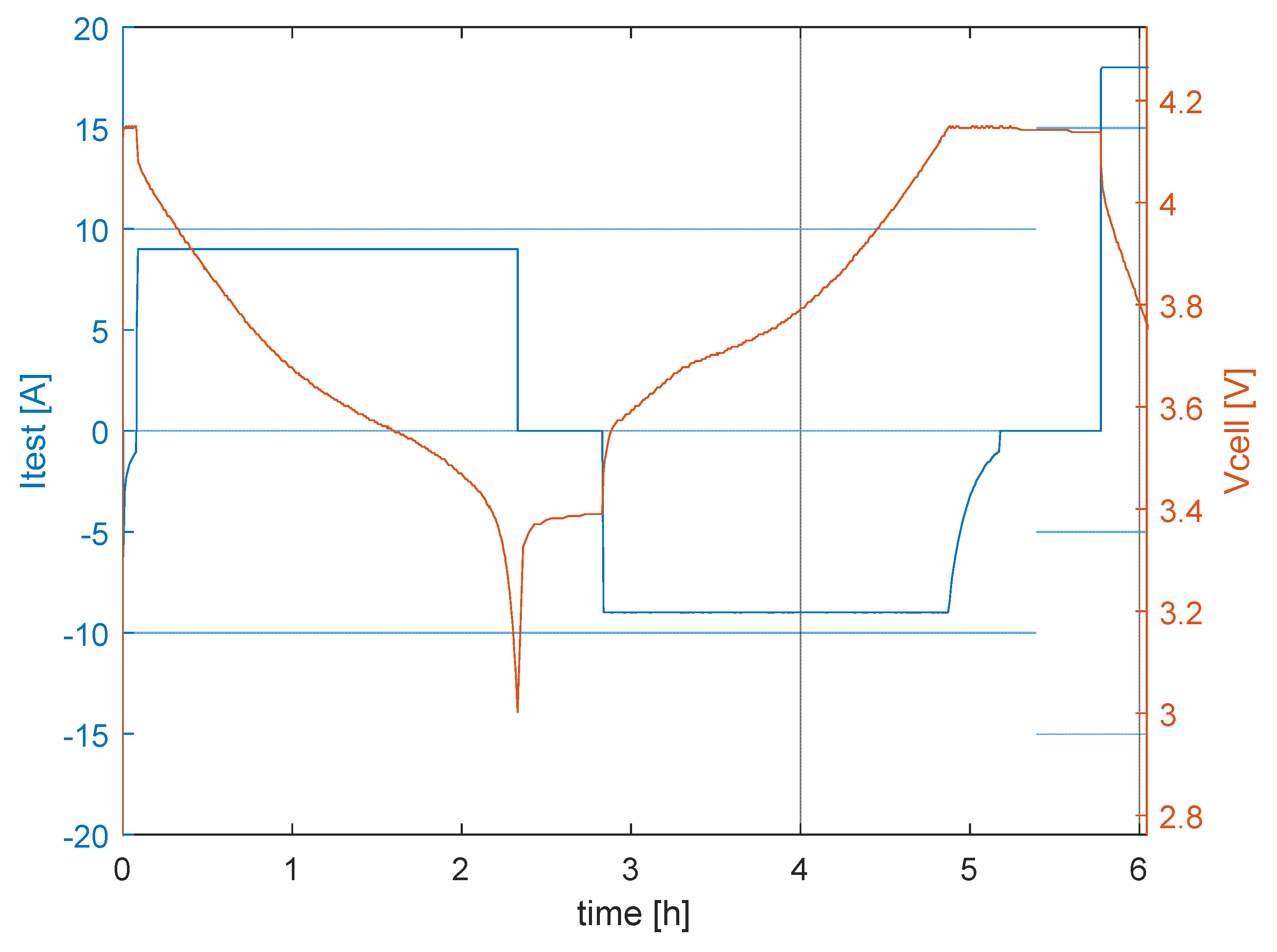
The capacity measurement test consists of measuring the capacity value of a cell, after a thermal stabilization pause, by using a standard cycle. The cell is discharged CC at I = 0.5 C, rested for 30 min, and then subjected to a CC-CV charge at I = 0.5 C up to SOC = 100%. The procedure is repeated for a current of 1 C. Each of these processes is interspersed with appropriately calibrated pauses. The test is repeated twice with each measurement session.
A typical discharge–charge profile for an applied current of 0.5 C, is reported in Figure 2. The current is calculated on the actual initial capacity value rather than on the 20 Ah nominal value. For all the tested cells, the initial capacity was always smaller than the nominal one, with an average value of 19 Ah, and a standard deviation for the population of 0.4 Ah.
3.2. Modeling of Cell Behavior
To compare the experimental results for life tests in which the definition of the cycle is different in the duration and depth of discharge, it is necessary to find a suitable parameter. It was therefore considered appropriate to analyze the capacity trend as a function of the cumulative charge, defined by the Equation (1):
where is the instantaneous current flowing through the cell. With this variable, the capacity trends for cells whose duty cycles have different depths of discharge can be compared.
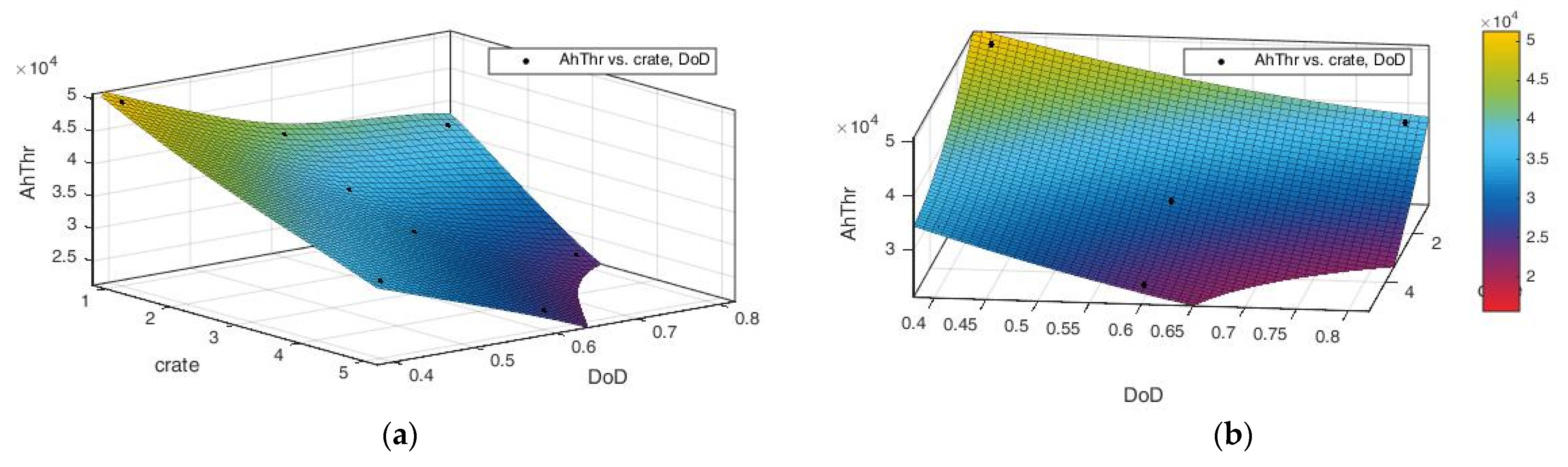
Figure 3 graphically shows the relationship between the amount of cumulative charge supplied until reaching the EOL condition (C/C0 = 0.8), and the stress factors analyzed for cells B1–B8. The experimental points are represented as black dots on the surface.
The curve was interpolated with a second-degree polynomial function with respect to the two independent variables, using the MatLab® Curve Fitting Toolbox. The value of R2 is very close to 1, but the value of the sum of squares due to error (SSE) is extremely high, which means that the model has a large random error component and that the fit is not useful for prediction.
3.2.1. Proposed Model
In its simplest form, an aging model consists of an empirical correlation between the observable quantities (capacity and/or internal resistance) as a function of time or cycles or cumulative charge, and various aging factors, such as temperature, current, and state of charge.
In the present study, we want to find a model that describes the change of the relative value of the battery capacity defined as in Formula (2):
where is the value of the initial (or nominal) capacity of the battery, and is the value of the capacity measured at a given time t, which is a function of the cumulative charge .
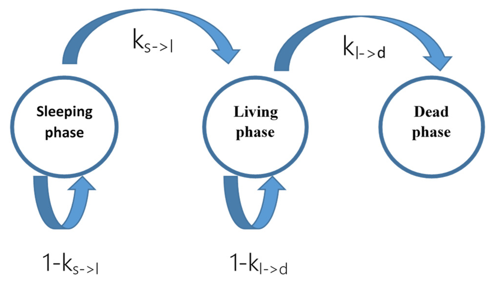
The proposed model has its base on the work by Risse et al. [28], in which the battery capacity degradation process is represented by a Markov chain consisting of three phases and four states, capable of capturing the phenomena that occur during the aging of a battery, including the initial formation. A Markov chain is a mathematical representation of a stochastic system that evolves with transitions from one state to another, according to certain probabilistic rules. In Markov chains, the transition probabilities do not depend on the system history. In the present work, we are not interested in the formation phase, so we can reduce the model to three phases: the sleeping phase , which represents the portion of the bound charge that can be converted into the active phase during cycling; the living phase , which represents the capacity immediately available; and the dead phase , which represents the portion of material no longer available for cycling. Once the active materials are transferred from the active state to the dead state, they can no longer be used in the charging and discharging processes. The dead state is thus an absorbing state. The system state is a combination of the three phases. The initial state is defined as the vector reported in (3):
At each step of the Markov process, each phase A evolves into phase B with probability , where is the probability of finding the system in state A and coincides with the fraction of the system that is in that state. is the conditional probability that the system passes from state A to state B, given that the system is in state A. The model describes the evolution of the fractions of the phases after a charge and discharge cycle by means of a suitable transition matrix (4):
where:
- is the transition probability between the living and dead phase;
- is the transition probability between the sleeping and living phase.
The Markov chain described by the transition matrix is stationary. Furthermore, the sum of all the elements of the state vector remains constant, ensuring the conservation of mass in the process. Figure 4 shows a graphical representation of the Markov process.
The state of the system at cycle n is represented by a column vector whose elements represent the fraction in the three different phases, as in (5):
Starting from the initial state (3), the transition from the n-th cycle to the n + 1-th cycle is obtained by multiplying the vector (5) by the transition matrix (4):
From the previous definitions (6), it can be deduced that the measured capacity is proportional to the fraction of the system state that is in the active phase. Applying Formula (5), the active phase after n cycles is given by Equation (7):
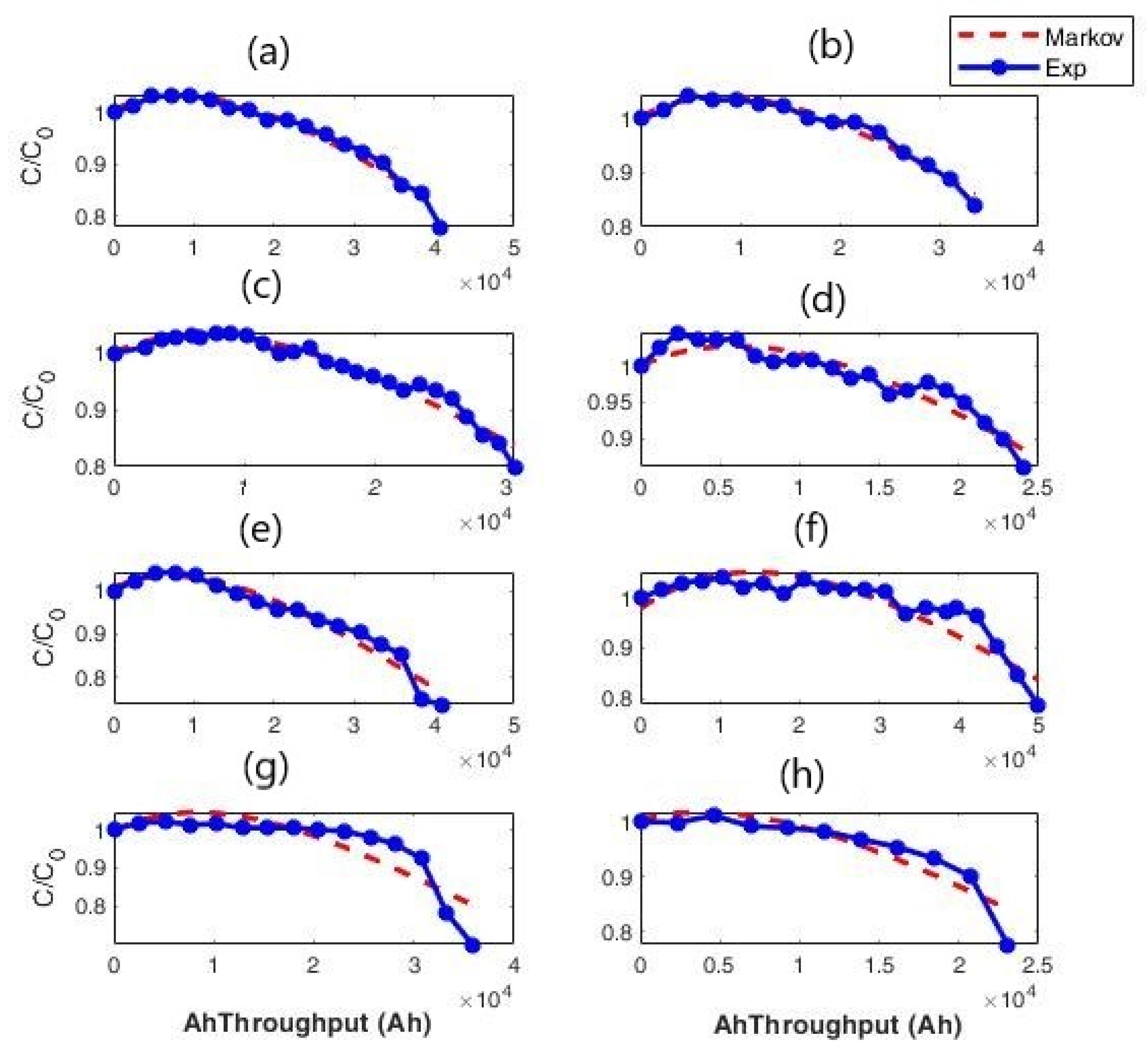
We fit the experimental data with the Markov model for cells number 1 to number 8. We find that the model can reproduce the degradation trend of the batteries only when the intensity of the applied stresses is not too high, while deviations are detected between the model fitting and the experimental data for higher intensities of stress. In particular, the model fails to reproduce the capacity degradation curve when it shows a variation in the slope that usually occurs as the strength of the applied stresses increases. As an example, we report the degradation curves (in blue) and the fitting of the Markov model (in red), in Figure 5, for all the cells, from number 1 to number 8.
As it can be seen from Figure 5, for the batteries with a lower stress intensity (the cells from 1 to 6), the Markov model can catch the main features of the experimental curve. However, the deviation from the experimental data is relevant in the case of the stronger stress (cells 7 and 8), especially toward the EOL.
In order to interpolate the experimental data, it is necessary to modify the model. In particular, to describe the knee present in the degradation curve, a transition probability has been introduced, which depends on the number of suitably defined cycles n. The transition matrix at cycle n is represented in Formula (8):
The transition matrix (8) reduces to that of the original Markov model when the term . Since the transition probability depends on the system history, the resulting model is non-Markovian. The state of the system is represented as before by the weighted combination of the three possible phases, as reported in (9):
The trend of the capacity is represented by the component (10) of the state that corresponds to the living phase :
Unlike the Markov model (3), for the introduced model it is not possible to find a closed analytic expression for , so it is necessary to resort to a numerical solution. A MatLab® curve fitting tool was used to solve the problem of determining the parameters of the transition matrix and of the initial phases’ value.
As model (8) contains the cycle number in its definition, it represents a discrete process. In order to compare the results for cells subjected to life tests with different ΔSOCs, it is necessary to appropriately quantize the cumulative charge, to obtain a suitably defined equivalent cycle. To this end, we consider the greatest common factor (GCF) among ΔSOCs. We then define the number of equivalent cycles (ECs) of each life test as the ratio between the ΔSOC value and GCF. In our case, we considered 3 ΔSOC: 40%, 60%, and 80%. The GCF is therefore 20%. Hence, the number of EC equals 2, 3, and 4 for each cycle at ΔSOC 40, 60, and 80%, respectively. Obviously, this is not the only quantization possible, but a different choice does not affect the validity of the model, as long as the transformation is linear, although it would lead to different results for the parameters.
We report the results obtained with this model for batteries 1–4 in Table 4.
The large number of parameters makes the interpretation of the results complex, and the model is more prone to numerical errors. The parameters and have intrinsic physical meaning for the cells since they represent the cells’ initial state, which should depend mainly on the chemical composition. Since the values for and are almost constant for all batteries, as is also the case in the original model (3), we replaced these parameters with the average values obtained, that is:
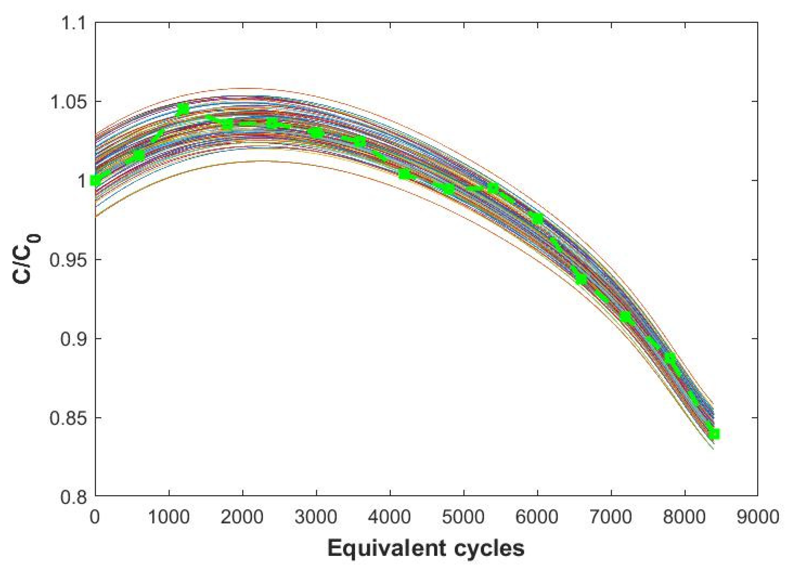
To verify the influence of the parameters and on the model output, we made a series of simulations, where the values of the two parameters are randomly chosen from two independent Gaussian distributions, with the average value centered in and , respectively, and the relative variance of 0.03. All the other parameters remained fixed at the value determined by the MatLab tool for = and = .
The results are shown in Figure 6, for the B2 battery. The simulation was made for a sample of 100 initial values of and and, for comparison, the experimental curve is also shown (in green with round symbols). It can be seen that the curves tend to converge as the number of equivalent cycles increases, indicating a limited influence of the values of the 2 parameters in the final part of life (variation of less than 2% in the cases examined). We can therefore consider that the error introduced by setting the value of and is irrelevant for determining the end of life.
In Table 5, we report the parameter values for batteries aged at different discharge currents for the model (8) with fixed and . The discrepancy for battery 2 in the trend for the value of exponent e (also visible in Table 4), can depend on the fact that the battery has undergone a swelling before the end of its life, to signal some type of internal malfunction that has been highlighted in the post-mortem analysis [29]. Further investigations are needed to verify if the deviations in the parameters can be related to the anomalies in the cells.
The same model was applied to the data obtained for the batteries aged with different ΔSOCs. The results are reported in Table 6.
As for the multiple stress tests carried out on batteries 7 and 8, the results obtained are shown in Table 7.
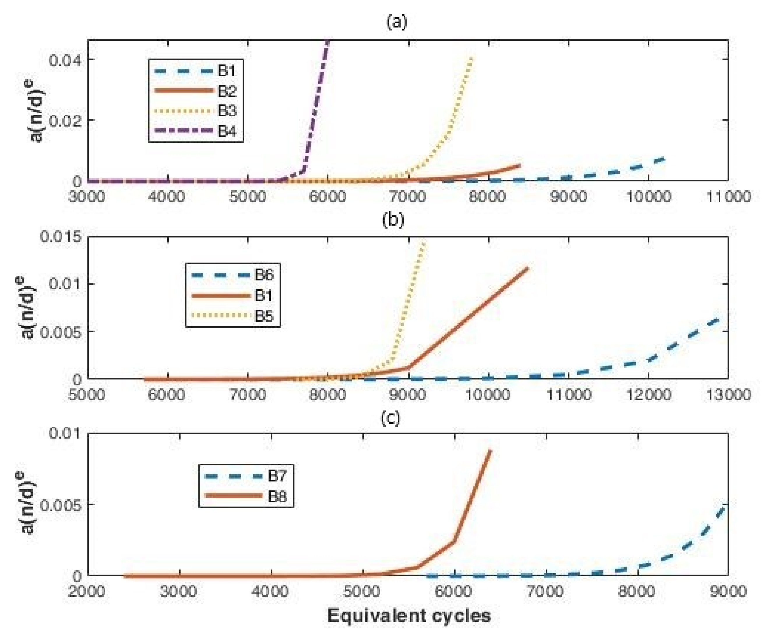
From Table 5 and Table 6, we can see that parameters b and c increase with an increasing stress amplitude. If this consideration also holds for combined stress, Table 7 shows that the stresses on battery number 7 are lower than the ones on battery number 8. This is also confirmed by the shorter life duration of battery number 8 (Figure 5). For the model purpose, it is more convenient to look at parameters a, d, and e as the combination that appears in the transition matrix (8). Figure 7 shows the profile for the exponential function as a function of the EC, n, for the cells: the top panel reports the cells with the different charge currents applied, the central panel the results for different DOD, and the bottom panel the results for cells number 7 and number 8.
We can see that all the curves tend to diverge with the increasing EC values, but the slope and the onset of the diverging behavior depend on the intensity of the applied stress. In particular, for cells number 7 and 8, the diverging behavior starts when the kink in the capacity curve as a function of the EC appears.
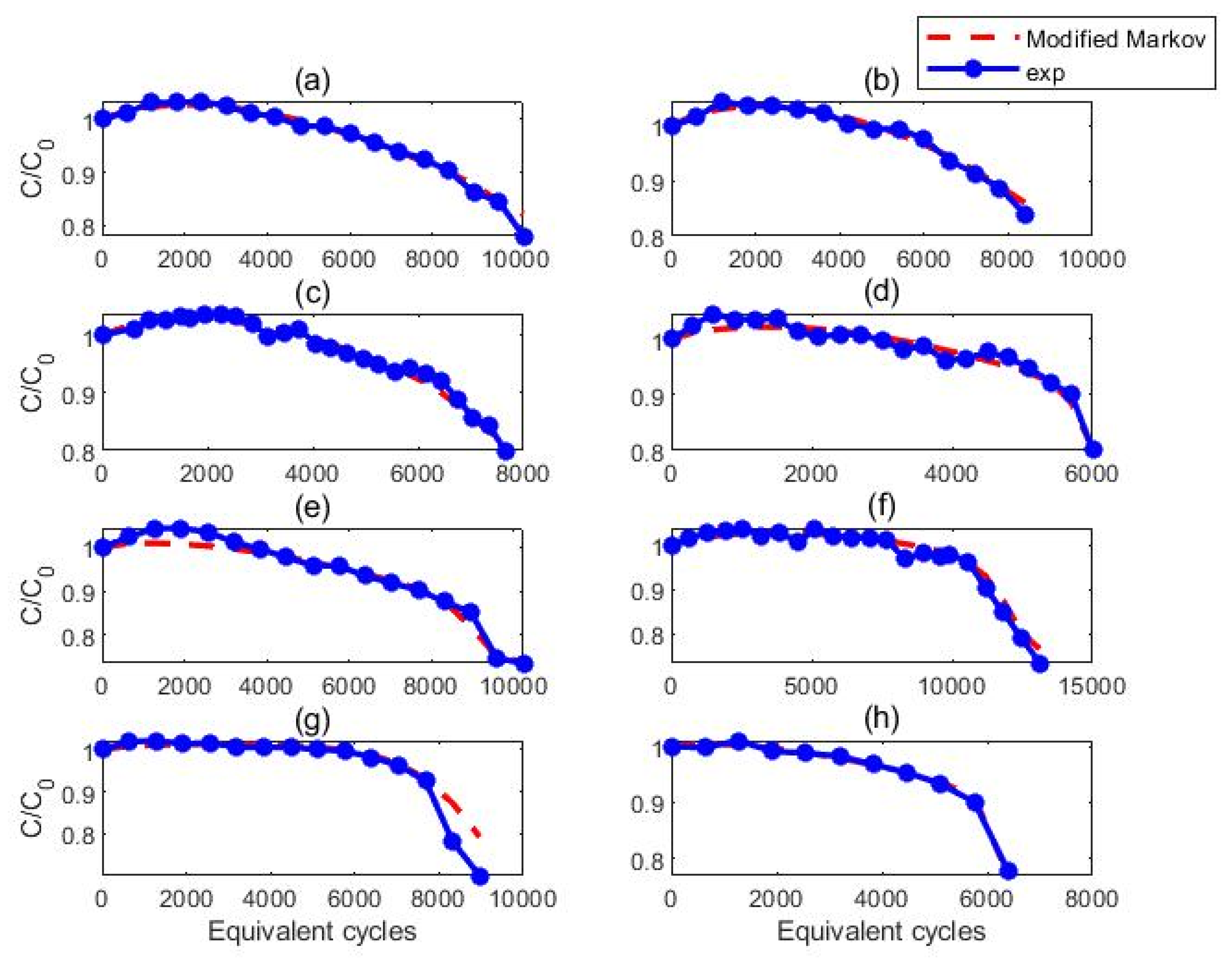
Figure 8 shows the comparison between the experimental trend of degradation curves and the results obtained from the model (8), as a function of the number of equivalent cycles.
Comparing it with the curves in Figure 5, it is clear that the modified model is able to reproduce the less regular behavior of cells subjected to high stress intensities. In particular, the knee present in the experimental curve is captured by the proposed model. Some deviations are present at the initial phase of the degradation curves and for battery 7 at the end of the curve, where the experimental data show a slope change that the model fails to reproduce.
3.2.2. Predictive Efficacy of the Model
In this section, we verify the model’s ability to predict the battery life when it is subjected to a work cycle composed of different stress intensities, using the results of the parameters obtained for the laboratory tests conducted with single stresses of predefined intensity. This procedure can be assimilated to an extrapolation of the model that uses the model parameters obtained for single stress tests, to simulate the capacity trend of a battery under a combined stresses test.
For this purpose, battery 9 was subjected to a life test whose aging cycle consists of the repetition of a macrocycle, composed as follows:
- (a)
- 8 cycles at a current rate of C-rate = 3 C and ΔSOC = 80%;
- (b)
- 10 cycles at a current rate of C-rate = 2 C and ΔSOC = 60%.
The macrocycle is composed of 8 × 4 = 32 equivalent cycles for the C-rate = 3 C phase and ΔSOC = 80%, and 10 × 3 = 30 equivalent cycles for the C-rate = 2 C phase and ΔSOC = 60%, for a total of 62 equivalent cycles per macrocycle.
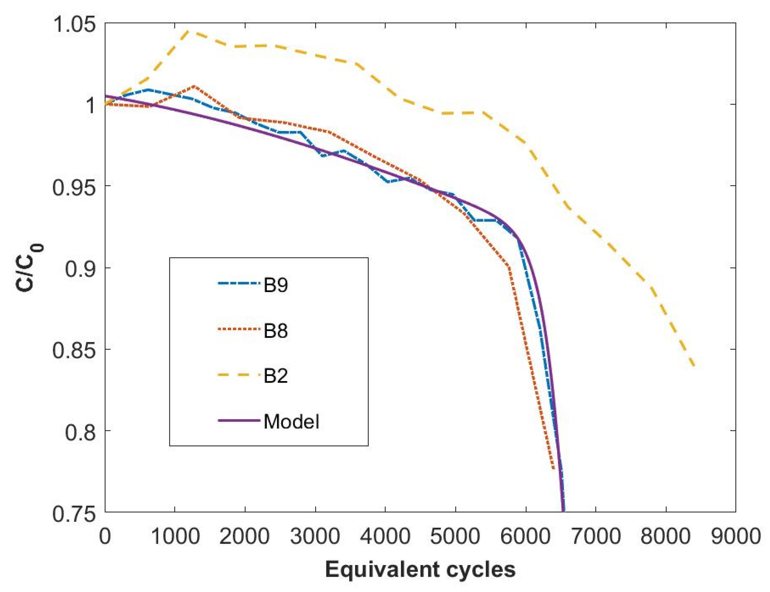
The results for the degradation curve of battery 9 are reported in Figure 9. For comparison, the experimental data of the batteries 8 and 2, which have been subjected to aging cycles of type (a) and (b), respectively, are also reported. If the effects of the different stress factors were added linearly, the degradation curve of battery 9 should be between those of batteries 8 and 2. However, the experimental data show that the curve is rather flattened on that of battery 8.
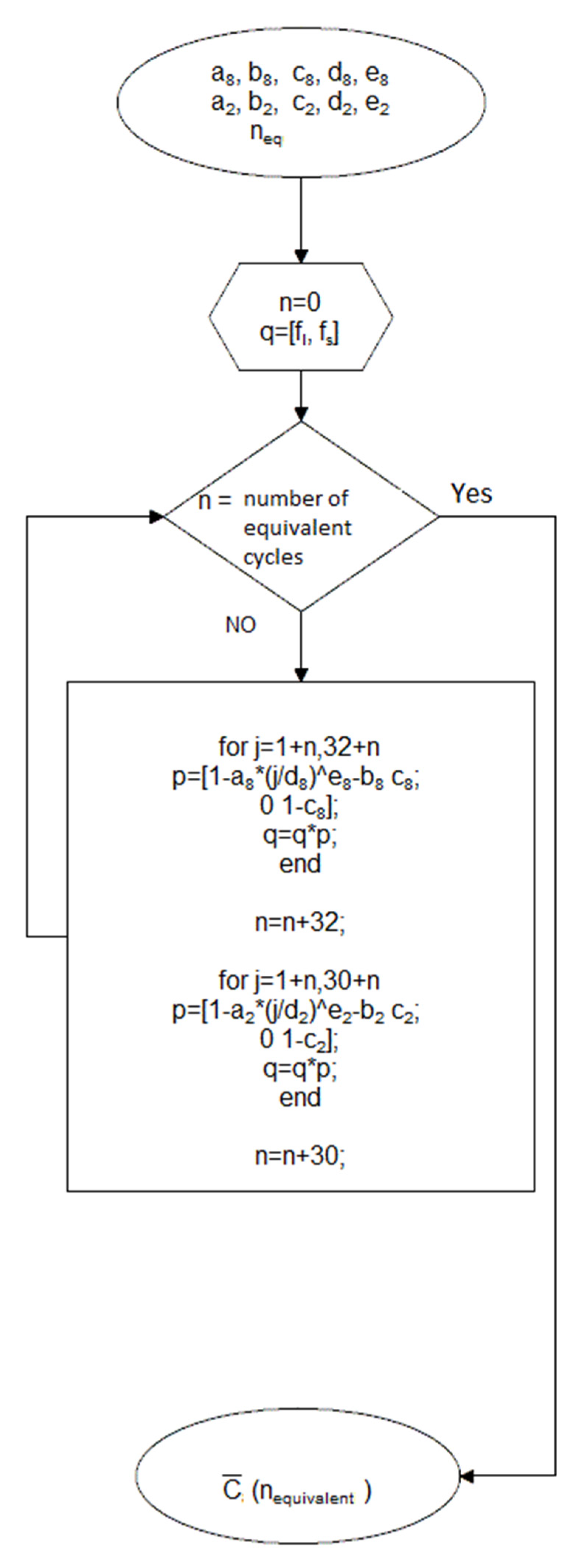
Furthermore, Figure 9 reports the results of the life simulation obtained by evaluating the parameter of model (8) on the experimental data of battery 9. The model reproduces well the experimental data. However, our aim is to estimate the capacity degradation for battery 9 using data from single stress tests. Figure 10 shows the flowchart of the program: as the input, we have the parameters from the experimental data for B2 and B8, as well as the fixed values of and . These represent the initial values of the vector q, which coincides with the initial state of the system whose third component, not shown, represents the dead phase. The parameters of the batteries B8 and B2 were appropriately inserted in the transition matrix (8), which was then used in the algorithm, represented by the loops shown in the flowchart. The output is the capacity of the battery after equivalent cycles. In this way, it is possible to obtain the simulation of the decay of the capacity of B9.
However, the capacity measurements are subject to many errors, which introduce a source of uncontrollable variability. These variations can arise from several sources:
- Inherent system uncertainties: due to the uncertainties in the manufacturing assembly and material properties, batteries can have different initial capacities. Each battery can also be individually affected by impurities or defects, which can lead to different aging rates [30].
- Measurement uncertainties: uncertainties are likely to arise from the background noise of measurement devices.
- Uncertainties in the operating environment: the rate of capacity fade can be affected by conditions of use, such as a shorter or longer shelf life before testing.
- Modeling uncertainties: the model is an approximation of battery degradation, which will lead to some modeling errors.
To partially obviate the random errors highlighted in points 1–3 above, we will analyze the model response when adding white noise to the model parameters. By analyzing the response for batteries 1–8, it is highlighted that the most dramatic effects for the evaluation of the battery life are due to the uncertainty on the accuracy of the parameters a, d, and e, which particularly affect the final part of the curve, therefore making it more difficult to estimate the life of the batteries.
By applying this process to all the parameters of batteries 2 and 8, and averaging the results obtained from the simulation, we obtain a curve that is closer to the experimental one in the end-of-life area, compared to that obtained using only the parameters extracted from the experimental results of B2 and B8. This result reinforces the fact that a more substantial statistic of experimental data can help to better identify the range of validity of the predictions. In Figure 11, the experimental curve (yellow), the extrapolated model output (blue), and the averaged output over the uncertain (red) are reported.
The percentage errors of the estimated cell life, compared to the number of equivalent cycles when the relative capacity has reached 0.78, are 2.8% for the extrapolation approach and 1.9% after averaging over the uncertainties.
The extrapolation approach allows the forecasting of the cycle life duration of a battery that undergoes an arbitrary duty cycle, using the parameters of model (8) for cells that underwent laboratory tests with determined stress applied.
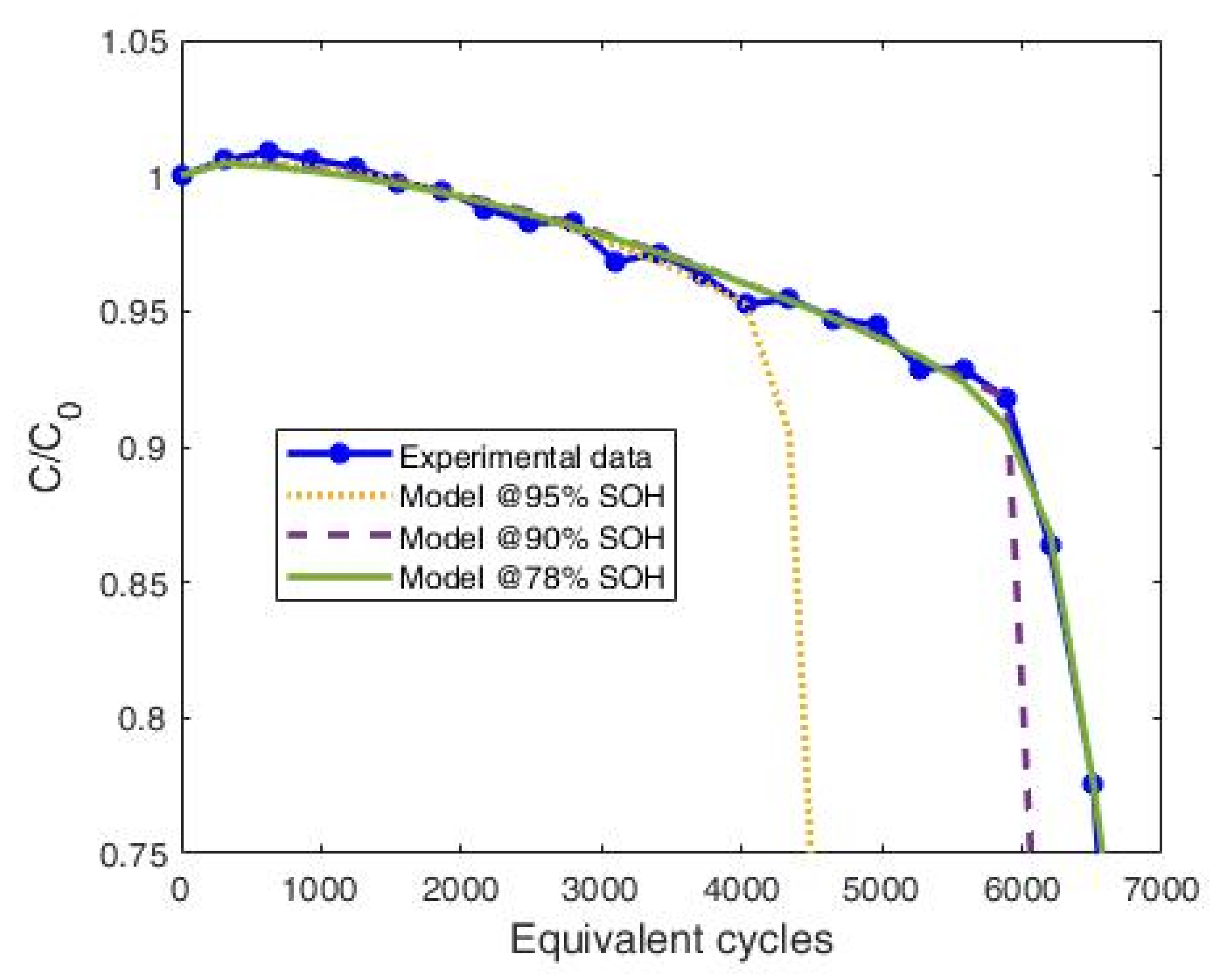
We compare the result of the proposed extrapolation approach with those obtained using the model (8), with parameters evaluated at different states of health (SOH). SOH is defined as the ratio between the capacity after n cycle and its initial value:
We evaluate model (8) parameters at 3 different SOH values: to 95, 90, and 78%.
Figure 12 shows the model output in the three cases and the experimental results for battery 9.
When the model parameters are evaluated using all the experimental data, until EOL, the modified Markov model is able to reproduce the curve, as expected. However, when the parameters are evaluated at 95% SOH, the error on the estimated and actual EOL number of equivalent cycles is around 44%, while, for 90% SOH, it is around 8%. In both cases, errors are larger than what obtained with the extrapolation approach.
4. Conclusions
The present study determines the effects that some stress factors, such as the depth of discharge and discharge current, have on the cycle life of lithium-ion batteries. To this end, life tests were conducted on battery cells. In particular, the cells under consideration use a technology based on lithium nickel cobalt manganese oxide (NCM) at the positive electrode and graphite at the negative electrode. Since the anode and cathode compositions are fundamental in the determination of the degradation process of lithium-ion cells, the results obtained during the study are strictly valid only for the analyzed technology. The results obtained are, in any case, in line with what is known in scientific literature, i.e., a faster degradation of batteries subjected to high discharge currents and greater depths of discharge.
We set up an experimental matrix to evaluate the impact of different stresses on the capacity fade. The data were used to study a methodology that would allow a reasonable life estimation even with a limited number of data available. We focused on a model that refers to the Markovian process structure, although it is not Markovian since the probability transition is dependent on the system history. This model describes the evolution of the system starting from an initial state consisting of different phases that evolves into successive states through a transition matrix. The three possible states are: dormant, in which the potential charge is found, but not directly available for cycling; active, in which the charge available for cycling is found; and dead, in which the charge is no longer available. The latter is an absorber state of the system, that is, the fraction of the system that reaches this state cannot pass into any other state. This model showed a good degree of fitting for the degradation curves of the analyzed cells, also managing to capture the knee present in some experimental results. As regards the ability to predict the trend of the capacity degradation curve, when analyzing a cell subjected to mixed stress starting from a grid of results obtained at constant stresses, the proposed model can estimate the battery life with an error of about 3% for NMC-graphite cells. The model parameters were extracted from the data sets obtained from the single tests for each stress. This limits the possibility to analyze the statistics of the stress effects and take into account the variability among batteries. Despite this lack of statistics on tests, the result for the prediction model can be regarded as satisfactory, although it is expected to improve by increasing the data statistics.
Author Contributions
Conceptualization, N.A.; methodology, N.A.; software, N.A.; validation, N.A., F.V. and V.S.; formal analysis, N.A.; investigation, N.A. and V.S.; resources, N.A. and F.V.; data curation, N.A.; writing—original draft preparation, N.A.; writing—review and editing, N.A. and F.V.; visualization, N.A. and V.S.; supervision, N.A.; project administration, N.A.; funding acquisition, N.A., F.V. and V.S. All authors have read and agreed to the published version of the manuscript.
Funding
This research was funded by the Italian Ministry of Economic Development, under the project PTR 2019—21 of the Electrical System Research, Project 1.7 “Technologies for the efficient penetration of the electric vector in end uses”, WP2 “Mobility”.
Institutional Review Board Statement
Not applicable.
Informed Consent Statement
Not applicable.
Data Availability Statement
The data presented in this study are openly available in Zenodo at 10.5281/zenodo.5785320].
Conflicts of Interest
The authors declare no conflict of interest.
References
- Venet, P.; Redondo-Iglesias, E. Batteries and Supercapacitors Aging. Batteries 2020, 6, 18. [Google Scholar] [CrossRef] [Green Version]
- Tang, X.; Zou, C.; Yao, K.; Lu, J.; Xia, Y.; Gao, F. Aging trajectory prediction for lithium-ion batteries via model migration and Bayesian Monte Carlo method. Appl. Energy 2019, 254, 113591. [Google Scholar] [CrossRef] [Green Version]
- Li, Y.; Liu, K.; Foley, A.M.; Zülke, A.; Berecibar, M.; Nanini-Maury, E.; Van Mierlo, J.; Hoster, H.E. Data-driven health estimation and lifetime prediction of lithium-ion batteries: A review. Renew. Sustain. Energy Rev. 2019, 113, 109254. [Google Scholar] [CrossRef]
- Zheng, Y.; Ouyang, M.; Lu, L.; Li, J. Understanding aging mechanisms in lithium-ion battery packs: From cell capacity loss to pack capacity evolution. J. Power Sources 2015, 278, 287–295. [Google Scholar] [CrossRef]
- Jafari, M.; Khan, K.; Gauchia, L. Deterministic models of Li-ion battery aging: It is a matter of scale. J. Energy Storage 2018, 20, 67–77. [Google Scholar] [CrossRef]
- Barré, A.; Deguilhem, B.; Grolleau, S.; Gérard, M.; Suard, F.; Riu, D. A review on lithium-ion battery ageing mechanisms and estimations for automotive applications. J. Power Sources 2013, 241, 680–689. [Google Scholar] [CrossRef] [Green Version]
- Mukhopadhyay, A.; Sheldon, B.W. Deformation and stress in electrode materials for Li-ion batteries. Prog. Mater. Sci. 2014, 63, 58–116. [Google Scholar] [CrossRef]
- Vetter, J.; Novák, P.; Wagner, M.R.; Veit, C.; Möller, K.-C.; Besenhard, J.O.; Winter, M.; Wohlfahrt-Mehrens, M.; Vogler, C.; Hammouche, A. Ageing mechanisms in lithium-ion batteries. J. Power Sources 2005, 147, 269–281. [Google Scholar] [CrossRef]
- Werner, D.; Paarmann, S.; Wetzel, T. Calendar Aging of Li-Ion Cells—Experimental Investigation and Empirical Correlation. Batteries 2021, 7, 28. [Google Scholar] [CrossRef]
- Redondo-Iglesias, E.; Venet, P.; Pelissier, S. Modelling Lithium-Ion Battery Ageing in Electric Vehicle Applications—Calendar and Cycling Ageing Combination Effects. Batteries 2020, 6, 14. [Google Scholar] [CrossRef] [Green Version]
- Leng, F.; Tan, C.; Pecht, M. Effect of Temperature on the Aging rate of Li Ion Battery Operating above Room Temperature. Sci. Rep. 2015, 5, 12967. [Google Scholar] [CrossRef] [Green Version]
- Alipour, M.; Ziebert, C.; Conte, F.V.; Kizilel, R. A Review on Temperature-Dependent Electrochemical Properties, Aging, and Performance of Lithium-Ion Cells. Batteries 2020, 6, 35. [Google Scholar] [CrossRef]
- Agubra, V.; Fergus, J. Lithium Ion Battery Anode Aging Mechanisms. Materials 2013, 6, 1310. [Google Scholar] [CrossRef] [Green Version]
- Bank, T.; Feldmann, J.; Klamor, S.; Bihn, S.; Sauer, D.U. Extensive aging analysis of high-power lithium titanate oxide batteries: Impact of the passive electrode effect. J. Power Sources 2020, 473, 228566. [Google Scholar] [CrossRef]
- Yu, R.; Banis, M.N.; Wang, C.; Wu, B.; Huang, Y.; Cao, S.; Li, J.; Jamil, S.; Lin, X.; Zhao, F.; et al. Tailoring bulk Li+ ion diffusion kinetics and surface lattice oxygen activity for high-performance lithium-rich manganese-based layered oxides. Energy Storage Mater. 2021, 37, 509–520. [Google Scholar] [CrossRef]
- International Organization for Standardization. Electrically Propelled Road Vehicles—Test Specification for Lithium-Ion Traction Battery Packs and Systems—Part 4: Performance Testing. Available online: https://www.iso.org/standard/71407.html (accessed on 26 May 2021).
- Ning, G.; Popov, B.N. Cycle life modeling of lithium-ion batteries. J. Electrochem. Soc. 2005, 151, A1584. [Google Scholar] [CrossRef] [Green Version]
- Doyle, M.; Fuller, T.F.; Newman, J. Modeling of galvanostatic charge and discharge of the lithium/polymer/insertion cell. J. Electrochem. Soc. 1993, 140, 1526–1533. [Google Scholar] [CrossRef]
- Doyle, M.; Newman, J. Analysis of capacity–rate data for lithium batteries using simplified models of the discharge process. J. Appl. Electrochem. 1997, 27, 846–856. [Google Scholar] [CrossRef]
- Fuller, T.F.; Doyle, M.; Newman, J. Relaxation phenomena in lithium-ion-insertion cells. J. Electrochem. Soc. 1994, 141, 982–990. [Google Scholar] [CrossRef] [Green Version]
- Madani, S.S.; Schaltz, E.; Kær, S.K. A Review of Different Electric Equivalent Circuit Models and Parameter Identification Methods of Lithium-Ion Batteries. ECS Trans. 2018, 87, 23–37. [Google Scholar] [CrossRef]
- Delacourt, C.; Safari, M. Mathematical Modeling of Aging of Li-Ion Batteries. In Physical Multiscale Modeling and Numerical Simulation of Electrochemical Devices for Energy Conversion and Storage. Green Energy and Technology; Franco, A., Doublet, M., Bessler, W., Eds.; Springer: London, UK, 2016; pp. 151–190. [Google Scholar]
- Andrenacci, N.; Sglavo, V.; Vellucci, F.; State of the Art of Aging Models for Lithium-Ion Cells. Application to the Case Study of Aged NMC cells in ENEA. Report RDS/ PAR2016/163. Available online: https://www.enea.it/it/Ricerca_sviluppo/lenergia/ricerca-di-sistema-elettrico/accordo-di-programma-MiSE-ENEA-2015-2017/trasmissione-e-distribuzione-dellenergia-elettrica/sistemi-di-accumulo-di-energia/report-2016 (accessed on 25 May 2021). (In Italian).
- Tamilselvi, S.; Gunasundari, S.; Karuppiah, N.; Abdul Razak, R.K.; Madhusudan, S.; Nagarajan, V.M.; Sathish, T.; Shamim, M.Z.M.; Saleel, C.A.; Afzal, A. A Review on Battery Modelling Techniques. Sustainability 2021, 13, 10042. [Google Scholar] [CrossRef]
- Chang, C.-Y.; Tulpule, P.; Rizzoni, G.; Zhang, W.; Du, X. A probabilistic approach for prognosis of battery pack aging. J. Power Sources 2017, 347, 57–68. [Google Scholar] [CrossRef] [Green Version]
- Jiang, L.; Xian, W.M.; Long, B.; Wang, H.J. Analysis of Data-Driven Prediction Algorithms for Lithium-Ion Batteries Remaining Useful Life. Adv. Mater. Res. 2013, 717, 390–395. [Google Scholar] [CrossRef]
- Chiodo, E.; Lauria, D.; Mottola, F.; Andrenacci, N. Online Bayes Estimation of Capacity Fading for Battery Lifetime Assessment. In Proceedings of the 2019 International Conference on Clean Electrical Power (ICCEP), Otranto, Italy, 2–4 July 2019; pp. 599–604. [Google Scholar]
- Risse, S.; Angioletti-Uberti, S.; Dzubiella, J.; Ballauff, M. Capacity fading in lithium/sulfur batteries: A linear four-state model. J. Power Sources 2014, 267, 648–654. [Google Scholar] [CrossRef]
- Bacaloni, A.; Insogna, S.; Di Bari, C.; Andrenacci, N.; Mazzaro, M.; Navarra, M.A. Characterization of Li-ion batteries for safety and health protection. Ital. J. Occup. Environ. Hyg. 2019, 10, 40–52. [Google Scholar]
- Harris, S.J.; Harris, D.J.; Li, C. Failure statistics for commercial lithium ion batteries: A study of 24 pouch cells. J. Power Sources 2017, 342, 589–597. [Google Scholar] [CrossRef] [Green Version]
Figure 1.
EiG PLB C020 cell.

Figure 2.
Typical discharge–charge profile for EiG PLB C020 cells.

Figure 3.
Graphical representation of the cumulative charge trend as a function of the C-rate and the depth of discharge of the life cycles. The same graph is shown for two different perspectives (a,b).
Figure 3.
Graphical representation of the cumulative charge trend as a function of the C-rate and the depth of discharge of the life cycles. The same graph is shown for two different perspectives (a,b).

Figure 4.
Graphical representation of the Markov model for the aging model.

Figure 5.
Comparison between the trend of the experimental and Markov degradation curve for cells 1–8. Blue line, diamond symbol: experimental data and red line square symbol: Markov fitting: (a) battery number 1; (b) battery number 2; (c) battery number 3; (d) battery number 4; (e) battery number 5; (f) battery number 6; (g) battery number 7; (h) battery number 8.

Figure 6.
Effects of the variation of fl0 and fs0 on the capacity trend as a function of the number of equivalent cycles. In green with round symbols: the experimental curve for B2.
Figure 6.
Effects of the variation of fl0 and fs0 on the capacity trend as a function of the number of equivalent cycles. In green with round symbols: the experimental curve for B2.

Figure 7.
Curves for the exponential term of the transition matrix (8), as a function of the equivalent cycles and for different cells: (a) comparison among cells from number 1 to 4; (b) comparison among cells number 6, 1 and 5; (c) comparison between cell number 7 and cell number 8.
Figure 7.
Curves for the exponential term of the transition matrix (8), as a function of the equivalent cycles and for different cells: (a) comparison among cells from number 1 to 4; (b) comparison among cells number 6, 1 and 5; (c) comparison between cell number 7 and cell number 8.

Figure 8.
Comparison between the experimental data and the model (8), as a function of the number of equivalent cycles: (a) battery number 1; (b) battery number 2; (c) battery number 3; (d) battery number 4; (e) battery number 5; (f) battery number 6; (g) battery number 7; (h) battery number 8.
Figure 8.
Comparison between the experimental data and the model (8), as a function of the number of equivalent cycles: (a) battery number 1; (b) battery number 2; (c) battery number 3; (d) battery number 4; (e) battery number 5; (f) battery number 6; (g) battery number 7; (h) battery number 8.

Figure 9.
Degradation curve of the capacity for cell B9 with respect to the number of equivalent cycles and the comparison between the predictions of the model (8). For comparison, the curves of batteries 8 and 2 are shown.
Figure 9.
Degradation curve of the capacity for cell B9 with respect to the number of equivalent cycles and the comparison between the predictions of the model (8). For comparison, the curves of batteries 8 and 2 are shown.

Figure 10.
Flowchart of the life span extrapolation method, based on transition matrix (8).

Figure 11.
Comparison between the experimental curve, the extrapolation of the modified Markov model and the simulation average.
Figure 11.
Comparison between the experimental curve, the extrapolation of the modified Markov model and the simulation average.

Figure 12.
Comparison among model (8) outputs for the parameters evaluated at a different SOH.


Table 1.
Main electric and operating characteristic of EiG PLB C020 cells.
| Cell Characteristic | Value |
|---|---|
| Nominal voltage | 3.65 V |
| Maximum voltage | 4.15 V |
| Minimum voltage | 2.5 V |
| Nominal capacity | 20 Ah |
| Maximum discharge current (continuous) | 5 C |
| Maximum discharge current (peak < 10 s) | 10 C |
| Operating temperature | −30 °C/+55 °C |
| Charging temperature | 0 °C/+40 °C |
| Storage temperature | −30 °C/+55 °C |
| Specific energy | 174 Wh/Kg |
| Volumetric energy density | 370 Wh/L |
| Specific power (DoD 50%, 10 s) | 2300 W/kg |
| Volumetric power density (DoD 50%, 10 s) | 4600 W/L |
| Storage temperature | −30 °C/+55 °C |
| Specific energy | 174 Wh/Kg |
| Volumetric energy density | 370 Wh/L |
Table 2.
Laboratory equipment used in the tests.
| Equipment | Name | Rating |
|---|---|---|
| Cycler | ELTRA E-8094 (double field) | V = 0–36 V; I = 280 A; Vmax = 36–52 V; I = 400 A |
| Cycler | ELTRA E-8376 (double field) | V = 0–35 V; I = 400 A; V = 36–350 V; I = 600 A |
| Cycler | ELTRA E-8325 | V = 0–20 V; I = 80 A (charge)–150A (discharge) |
| Cycler | DIGATRON 80V 8 channels | V = 0–100 V; I = 50 A |
| Cycler | Maccor Series 4000 48 channels | V = 0–5 V; I = 5 A |
| Cycler | Maccor Series 4000 8 channels | V = 0–80 V; I = 50 A |
| Climatic chamber | Angelantoni EOS 1000 | −40 °C, +180 °C; U.R. 15–98% |
| Climatic chamber | Angelantoni UY 2250 SP | −40 °C, +180 °C; U.R. 15–98% |
| Climatic chamber | Angelantoni DY 1200C EX | −60 °C, +150 °C; U.R. 15–98% |
Table 3.
Summary of the test parameters for the cells.
| Test Number | Discharge Current (C-Rate) | ΔSOC = SOCin − SOCfin | Cycle between Control Tests |
|---|---|---|---|
| 1 | 1 C | 60 = 80−20 | 200 |
| 2 | 2 C | 60 = 80−20 | 200 |
| 3 | 3 C | 60 = 80−20 | 100 1 |
| 4 | 5 C | 60 = 80−20 | 100 |
| 5 | 1 C | 80 = 90−10 | 160 |
| 6 | 1 C | 40 = 70−30 | 320 |
| 7 | 5 C | 40 = 70−30 | 320 |
| 8 | 3 C | 80 = 90−10 | 160 |
| 9 | 8 × 3C@80%DOD + 10 × 2C@60%DOD | 80 = 90−10, 40 = 70−30 | 90 |
1 First control test after 200 cycles.
Table 4.
Parameters of the model (8) for batteries with a different C-rate as a function of the number of equivalent cycles.
Table 4.
Parameters of the model (8) for batteries with a different C-rate as a function of the number of equivalent cycles.
| Model Parameters | B1 | B2 | B3 | B4 |
|---|---|---|---|---|
| fl | 1.01 | 1.008 | 1.009 | 1.04 |
| fs | 1.114 | 1.016 | 1.036 | 1.185 |
| a | 0.0001846 | 0.0003431 | 0.000104 | 0.0001705 |
| b | 8.733 × 10⁻⁵ | 9.388 × 10⁻⁵ | 0.000107 | 9.571 × 10⁻⁵ |
| c | 9.667 × 10⁻⁵ | 0.0001235 | 0.0001035 | 8.01 × 10⁻⁵ |
| d | 1.003 × 10⁴ | 9200 | 7138 | 5609 |
| e | 14.86 | 10.98 | 15.88 | 26.54 |
| R2 | 0.994 | 0.9873 | 0.9842 | 0.9496 |
Table 5.
Model parameter with fixed values for and , for batteries with a different C-rate.
| Model Parameters | B1 | B2 | B3 | B4 |
|---|---|---|---|---|
| a | 0.0001713 | 0.0003379 | 0.0001123 | 0.0001705 |
| b | 8.847 × 10⁻⁵ | 9.762 × 10⁻⁵ | 0.000112 | 0.0001189 |
| c | 0.0001018 | 0.0001183 | 0.0001298 | 0.0001331 |
| d | 9970 | 9175 | 7172 | 5669 |
| e | 16.43 | 10.19 | 16.74 | 36.66 |
| R2 | 0.994 | 0.9873 | 0.9842 | 0.9496 |
Table 6.
Model parameter with fixed values for f_l0 and f_s0, for batteries with a different ΔSOC.
| Model Parameters | B6 | B1 | B5 |
|---|---|---|---|
| a | 0.0001013 | 0.0001713 | 0.0001379 |
| b | 4.993 × 10⁻⁵ | 8.847 × 10⁻⁵ | 9.817 × 10⁻⁵ |
| c | 5.802 × 10⁻⁵ | 0.0001018 | 0.000112 |
| d | 1.139 × 10⁴ | 9970 | 9844 |
| e | 8.65 | 16.43 | 44.15 |
| R2 | 0.9777 | 0.994 | 0.9844 |
Table 7.
Model parameter with fixed values for f_l0 and f_s0, for batteries with multiple stress.
| Model Parameters | B7 | B8 |
|---|---|---|
| a | 9.021 × 10⁻⁵ | 0.0002348 |
| b | 4.396 × 10⁻⁵ | 9.183 × 10⁻⁵ |
| c | 4.583 × 10⁻⁵ | 8.713 × 10⁻⁵ |
| d | 7202 | 6086 |
| e | 18.203 | 17.31 |
| R2 | 0.9818 | 0.9964 |
Publisher’s Note: MDPI stays neutral with regard to jurisdictional claims in published maps and institutional affiliations. |
© 2021 by the authors. Licensee MDPI, Basel, Switzerland. This article is an open access article distributed under the terms and conditions of the Creative Commons Attribution (CC BY) license (https://creativecommons.org/licenses/by/4.0/).
Share and Cite
MDPI and ACS Style
Andrenacci, N.; Vellucci, F.; Sglavo, V. The Battery Life Estimation of a Battery under Different Stress Conditions. Batteries 2021, 7, 88. https://doi.org/10.3390/batteries7040088
AMA Style
Andrenacci N, Vellucci F, Sglavo V. The Battery Life Estimation of a Battery under Different Stress Conditions. Batteries. 2021; 7(4):88. https://doi.org/10.3390/batteries7040088
Chicago/Turabian StyleAndrenacci, Natascia, Francesco Vellucci, and Vincenzo Sglavo. 2021. "The Battery Life Estimation of a Battery under Different Stress Conditions" Batteries 7, no. 4: 88. https://doi.org/10.3390/batteries7040088
Note that from the first issue of 2016, this journal uses article numbers instead of page numbers. See further details here.