Applications of Skew Models Using Generalized Logistic Distribution

Abstract

We use the skew distribution generation procedure proposed by Azzalini [Scand. J. Stat., 1985, 12, 171–178] to create three new probability distribution functions. These models make use of normal, student-t and generalized logistic distribution, see Rathie and Swamee [Technical Research Report No. 07/2006. Department of Statistics, University of Brasilia: Brasilia, Brazil, 2006]. Expressions for the moments about origin are derived. Graphical illustrations are also provided. The distributions derived in this paper can be seen as generalizations of the distributions given by Nadarajah and Kotz [Acta Appl. Math., 2006, 91, 1–37]. Applications with unimodal and bimodal data are given to illustrate the applicability of the results derived in this paper. The applications include the analysis of the following data sets: (a) spending on public education in various countries in 2003; (b) total expenditure on health in 2009 in various countries and (c) waiting time between eruptions of the Old Faithful Geyser in the Yellow Stone National Park, Wyoming, USA. We compare the fit of the distributions introduced in this paper with the distributions given by Nadarajah and Kotz [Acta Appl. Math., 2006, 91, 1–37]. The results show that our distributions, in general, fit better the data sets. The general R codes for fitting the distributions introduced in this paper are given in Appendix A.

1. Introduction

The skew symmetric models have been considered by several researchers. Skew normal distribution is a classical example. Abtahi et al. [1] constructed skew student-t and skew Cauchy distributions. Recently, Rathie et al. [2,3] introduced a system of univariate skew distributions by utilizing Rathie and Swamee [4] generalized logistic distribution. For certain values of the parameters, this skew distribution approximates nicely the skew normal distribution. Recently, Gupta and Kundu [5] defined and studied two generalizations of the logistic distribution by introducing skewness parameters. In this paper we use Azzalini’s formula to generate new asymmetric distributions by using the Generalized Logistic, Normal and Student-t distributions. The distributions are Skew Normal-Generalized Logistic (Skew Normal-GL), Skew Generalized Logistic-Normal (Skew GL-Normal), Skew Student-t-Generalized Logistic (Skew t-GL) and Skew Generalized Logistic-Student-t (Skew GL-t). The models Skew GL-t and Skew GL-Normal generated by using $f(.)$ as define by the Equation (1) are bimodal for values of a close to 0, it is important to note that the values of the parameters determining uni/bi modal shapes are yet to be investigated.

We apply these distributions to three real data sets (expenditure on education, expenditure on health and waiting time between eruptions of the Old Faithful Geyser. We compare the fit of the distributions introduced in this paper with the distributions given by Nadarajah and Kotz [6], the results show that: (1) our distributions, in general, fit better the data sets; (2) The Skew GL-Normal, Skew GL-t, Skew Normal-GL and Skew t-GL distributions can be used to model symmetrical and asymmetrical unimodal data; (3) The Skew GL-Normal and Skew GL-t distributions can be used to adjust bimodal symmetrical and asymmetrical data, offering good fits, showing a high flexibility which is not common in the literature on probability distributions, which are mostly unimodal. This may be very important in practical applications; (4) The distributions are robust to numerical calculations in practical applications. The general R codes for fitting the distributions introduced in this paper are given in Appendix A.

The paper is organized as follows. In Section 2, we introduce the Skew Normal-GL, Skew GL-Normal, Skew t-GL and Skew GL-t distributions and we obtained the mathematical expressions for the moments, respectively. In Section 3, we apply the new distributions in three real data sets. Finally, in Section 4, we point out some final considerations of the results obtained in this paper.

We conclude this introduction section with some results which will be useful in the subsequent sections of this paper.

1.1. Generalized Logistic Distribution

We start by defining the symmetric generalized logistic density function and its cumulative distribution function studied recently by Rathie and Swamee [4]:

$$f\left(x\right)=\frac{\left[a+{b(1+p)\left|x\right|}^p\right]exp\left[-x\left(a+{b\left|x\right|}^p\right)\right]}{{\left\{exp\left[-x\left(a+{b\left|x\right|}^p\right)\right]+1\right\}}^2},$$

(1)

$$F\left(x\right)={\left\{exp\left[-x\left(a+{b\left|x\right|}^p\right)\right]+1\right\}}^{-1},$$

(2)

where $x\in \mathbb{R},a\ge 0,b\ge 0,p\ge 0$ (with a and b are not zero simultaneously), and $\mathbb{R}$ is the set of real numbers. For the values $a=1.59413$, $b=0.07443$ and $p=1.939$, this distribution approximates very well the normal distribution with a maximum error of $4\times {10}^{-4}$ at $x=0$ for the density function and $7.757\times {10}^{-5}$ at $x=2.81$ for the distribution function. For approximations to Student-t distribution, see Rathie et al. [3]. The case $a=0$ was studied, and applied to a civil engineering problem by Swamee and Rathie [7]. In the recent review article on univariate normal distribution, Rathie [8] pointed out that the generalized logistic distribution defined in (1) and (2) is invertible and that the approximation to the normal distribution is important for practical applications.

1.2. Azzalini’s Skew Distribution

Azzalini [9] obtained the following skew density function:

$$h\left(x\right)=2f\left(x\right)G\left(w\right(x\left)\right)(-\infty <x<\infty ),$$

(3)

where $f\left(x\right)$ is a symmetric probability density function about the origin, $G\left(x\right)$ is the cumulative distribution function of a symmetric density function about the origin, and $w\left(x\right)$ is an odd function of x. In this paper, we take $w\left(x\right)=cx$, $c\in \mathbb{R}$.

1.3. Moments

It is easy to calculate the n-th moments of $h\left(x\right)$ given in (3) with $w\left(x\right)=cx$, $c\in \mathbb{R}$, which are

$$E\left(X^n\right)=2{\int }_0^{\infty }{x}^{n}f\left(x\right)dx,$$

(4)

when n is even, and

$$E\left(X^n\right)=4{\int }_0^{\infty }{x}^{n}f\left(x\right)G\left(cx\right)dx-2{\int }_0^{\infty }{x}^{n}f\left(x\right)dx,$$

(5)

when n is odd.

1.4. Generalized Hypergeometric Function

The H-function, which is a generalization of Meijer’s G function, is given below

$$\begin{array}{c}{H}_{p,q}^{m,n}\left[x|\begin{array}{c}(a_1,A_1),...,(a_n,A_n),(a_{n+1},A_{n+1}),...,(a_p,A_p)\\ (b_1,B_1),...,(b_n,B_n),(b_{n+1},B_{n+1}),...,(b_p,B_p)\end{array}\right]=\hfill \\ =\frac{1}{2\pi i}{\int }_L\frac{{\prod }_{j=1}^m\mathsf{\Gamma }(b_j-B_{j}s){\prod }_{j=1}^n\mathsf{\Gamma }(1-a_j+A_{j}s)}{{\prod }_{j=m+1}^q\mathsf{\Gamma }(1-b_j+B_{j}s){\prod }_{j=n+1}^p\mathsf{\Gamma }(a_j-A_{j}s)}{x}^{s}ds.\hfill \end{array}$$

(6)

As a special case, we have

$$H_{p,q}^{m,n}\left[x|\begin{array}{c}(a_1,1),...,(a_p,1)\\ (b_1,1),...,(b_p,1)\end{array}\right]=G_{p,q}^{m,n}\left[x|\begin{array}{c}{a}_1,...,a_p\\ b_1,...,b_p\end{array}\right].$$

(7)

For details, see Luke [10], Springer [11], or Mathai et al. [12].

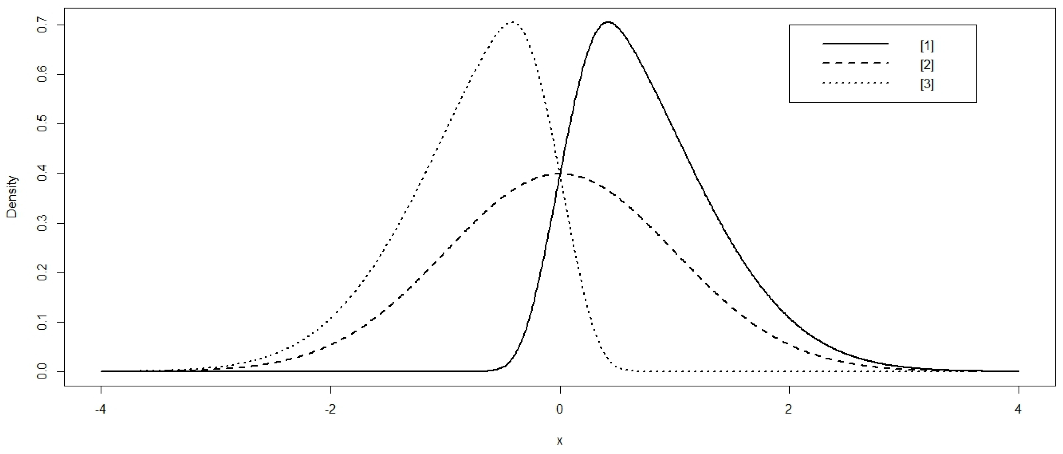
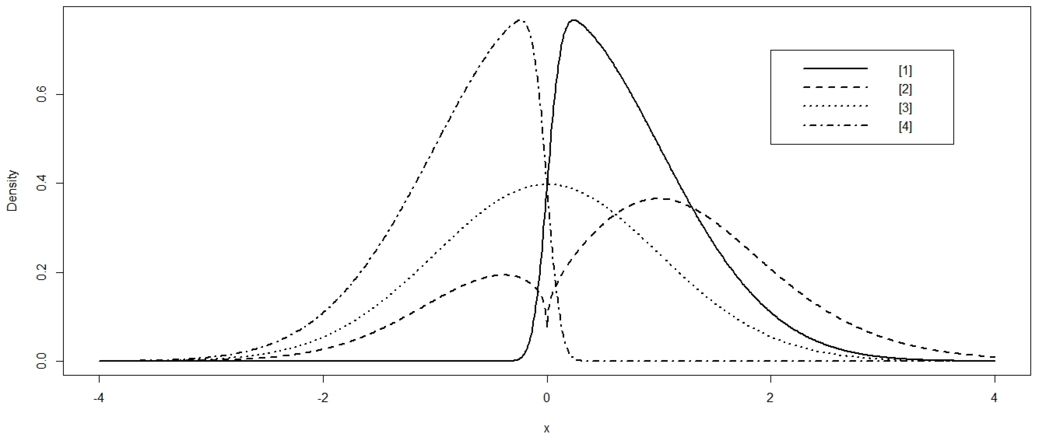
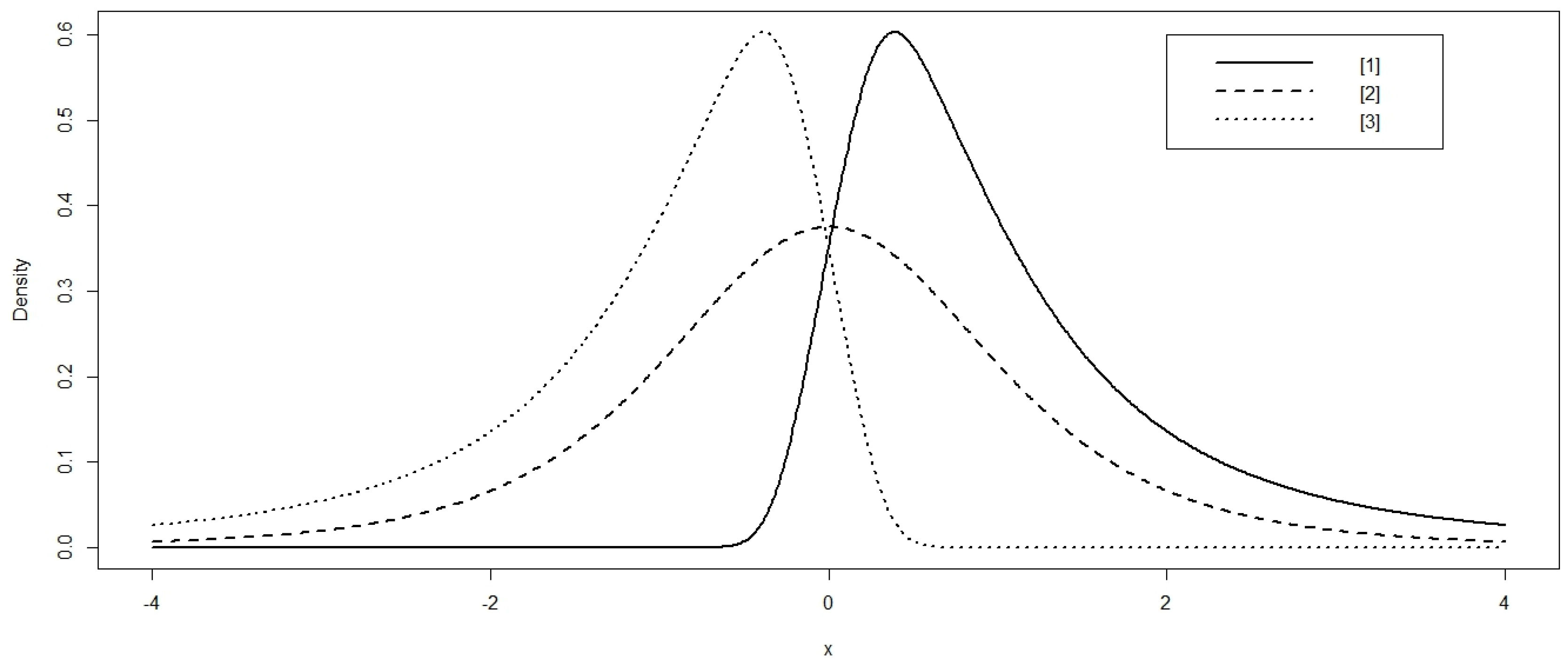
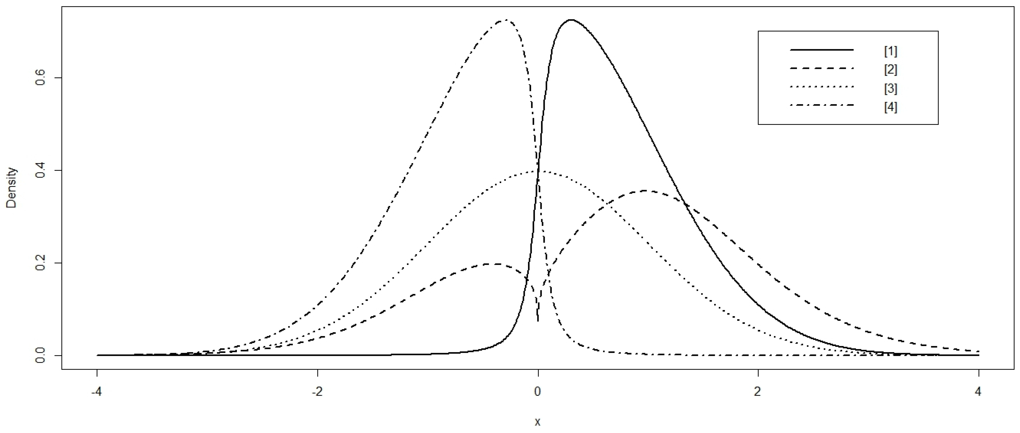
2. Skew Distributions

2.1. Skew Normal-Generalized Logistic Distribution

The skew normal-generalized logistic distribution (Skew Normal-GL), using (3), with $f\left(x\right)$ standard normal and $G\left(x\right)$ given in Equation (2) is defined by

$$h\left(x\right)=\sqrt{\frac{2}{\pi }}\frac{exp\left[\frac{-x^2}{2}\right]}{\left\{exp\left[-cx\left(a+b{\left|cx\right|}^p\right)\right]+1\right\}}(-\infty <x<\infty ).$$

(8)

In order that (8) is identifiable, we can rewrite it in the following form:

$$h\left(x\right)=\sqrt{\frac{2}{\pi }}\frac{exp\left[\frac{-x^2}{2}\right]}{\left\{exp\left[-x\left(A+B{\left|x\right|}^p\right)\right]+1\right\}}(-\infty <x<\infty ),$$

(9)

where $A=ac\in \mathbb{R}$ and $B={bc\left|c\right|}^p\in \mathbb{R}$. Plots for probability density function (9), varying some values of A, B and p, to show different forms of the Skew Normal-GL distribution are illustrated in Figure 1. We can see that the density has symmetric, asymmetric to the left and asymmetric to the right behavior, which may be important for practical purposes.

In the next subsection, we obtain n-th moments. For $B=0$, our results give alternative expressions for the results obtained earlier by Nadarajah and Kotz [6].

Moments

The n-th moments of (9) are

$$E\left(X^n\right)=\sqrt{\frac{2^n}{\pi }}\mathsf{\Gamma }\left(\frac{n+1}{2}\right),$$

(10)

for even values of n. For odd values of n, on using ${(1+y)}^{-1}={\sum }_{r=0}^{\infty }{(-y)}^r$, one gets

$$\begin{array}{cc}\hfill E\left(X^n\right)& =\frac{4}{\sqrt{2\pi }}\sum _{r=1}^{\infty }{(-1)}^r\sum _{k=0}^{\infty }\frac{{(-rB)}^k}{k!}\frac{{\left(rA\right)}^{-(p+1)k-n-1}}{2}\times \hfill \\ & H_{1,1}^{1,1}\left[\frac{1}{rA\sqrt{2}}|\begin{array}{c}(-(p+1)k-n,1)\\ (0,\frac{1}{2})\end{array}\right]+\left(2-\sqrt{2\pi }\right)\sqrt{\frac{2^n}{\pi }}\mathsf{\Gamma }\left(\frac{n+1}{2}\right).\hfill \end{array}$$

(11)

2.2. Skew Generalized Logistic-Normal Distribution

This section deals with the skew generalized logistic-normal distribution (Skew GL-Normal) defined below in (13). Moments about origin are obtained. The skew generalized logistic-normal distribution, using (3), with $f\left(x\right)$ given in (1) and

$$G\left(x\right)=\frac{1}{2}\left\{1+\frac{x}{\sqrt{2\pi }}{G}_{1,2}^{1,1}\left[\frac{x^2}{2}|\begin{array}{c}\frac{1}{2}\\ 0,\frac{-1}{2}\end{array}\right]\right\}(-\infty <x<\infty ),$$

(12)

is defined by

$$\begin{array}{c}\hfill h\left(x\right)=2\frac{\left[a+{b(1+p)\left|x\right|}^p\right]exp\left[-x\left(a+b{\left|x\right|}^p\right)\right]}{{\left\{exp\left[-x\left(a+{b\left|x\right|}^p\right)\right]+1\right\}}^2}G\left(cx\right)(-\infty <x<\infty ).\end{array}$$

(13)

Plots for probability density function (13), varying some values of a, b, p and c, to show different forms of the Skew GL-Normal distribution are illustrated in Figure 2. As in Skew Normal-GL distribution, the density has symmetric, asymmetric to the left and asymmetric to the right behavior. It is interesting to note that, for values of parameter a near to zero, the Skew GL-Normal distribution has a bimodal shape, which may be very important in practical applications.

In the next subsection, we obtain the moments of Skew GL-Normal distribution . For $b=0$, the results of this section give alternative expressions for the results obtained earlier by Nadarajah and Kotz [6].

Moments

Using (4) the n-th moments of (13) for even values of n has been calculated earlier by Rathie and Swamee [4], and are given by

$$E\left(X^n\right)=2\sum _{r=0}^{\infty }{(-1)}^r(1+r)\left[a{I}_{h,r}+b(1+p)I_{h+p,r}\right],$$

(14)

where

$$\begin{array}{cc}\hfill I_{\alpha ,r}& ={\int }_0^{\infty }{x}^{\alpha }exp\left[-(1+r)x\left(a+b{x}^p\right)\right]dx\hfill \\ & ={\left[a(1+r)\right]}^{-\alpha -1}{H}_{1,1}^{1,1}\left[\frac{a^{p+1}{(1+r)}^p}{b}|\begin{array}{c}(1,1)\\ (\alpha +1,p+1)\end{array}\right].\hfill \end{array}$$

(15)

For odd values of n, on using (7),

$$E\left(X^n\right)=\frac{4c}{\sqrt{2\pi }}\sum _{r=0}^{\infty }{(-1)}^r(1+r)\left[a{L}_{n+1,a(1+r)}+b(1+p)L_{n+p+1,a(1+r)}\right],$$

(16)

where

$$\begin{array}{cc}\hfill L_{\alpha ,\theta }& =\frac{2^{\alpha }}{\sqrt{\pi }{\theta }^{\alpha +1}}\sum _{k=0}^{\infty }{\left(\frac{-2^{p+1}(1+r)b}{{\theta }^{p+1}}\right)}^k\times \hfill \\ & \frac{1}{k!}{G}_{3,2}^{1,3}\left[\frac{2c^2}{{\theta }^2}|\begin{array}{c}-\frac{1}{2},\frac{1-\alpha -k(p+1)}{2},\frac{-\alpha -k(p+1)}{2}\\ 0,-\frac{1}{2}\end{array}\right].\hfill \end{array}$$

(17)

2.3. Skew Student-t-Generalized Logistic Distribution

The skew student-t-generalized logistic distribution (Skew t-GL), using Azzalini’s formula, is defined by

$$h\left(x\right)=\frac{2}{\sqrt{v}B\left(v/2,1/2\right)}{\left(1+\frac{x^2}{v}\right)}^{\frac{-(1+v)}{2}}{\left\{1+exp\left[-cx\left(a+{b\left|cx\right|}^p\right)\right]\right\}}^{-1},$$

(18)

for $-\infty <x<\infty$ and $v>0$. As before, taking $A_1=ac\in \mathbb{R}$ and $B_1=bc{\left|c\right|}^p\in \mathbb{R}$, (18) can be rewritten as

$$h\left(x\right)=\frac{2}{\sqrt{v}B\left(v/2,1/2\right)}{\left(1+\frac{x^2}{v}\right)}^{\frac{-(1+v)}{2}}{\left\{1+exp\left[-x\left(A_1+B_1{\left|x\right|}^p\right)\right]\right\}}^{-1},$$

(19)

for $-\infty <x<\infty$, $v>0$ and $B(.)$ is the Beta function, defined by $B(a,b)=\frac{\mathsf{\Gamma }\left(a\right)\mathsf{\Gamma }\left(b\right)}{\mathsf{\Gamma }(a+b)}$. Plots for probability density function (19), varying some values of $A_1$, $B_1$, p and v, showing different unimodal forms of the Skew t-GL distribution are illustrated in Figure 3. We can see that the density also has symmetric, asymmetric to the left and asymmetric to the right behavior. However, the Skew t-GL distribution has heavy tails.

In the next subsection, moments of the Skew t-GL distribution (19) are obtained.

Moments

The n-th moments of (19), using (4), are given by

$$E\left(X^n\right)=\frac{1}{\sqrt{\pi }\mathsf{\Gamma }(v/2)}\left[\mathsf{\Gamma }\left(\frac{v-n}{2}\right)\mathsf{\Gamma }\left(\frac{1+n}{2}\right)v^{n/2}\right],$$

(20)

if n is an even integer, and $0<n<v$. For odd integer n, and using the equation (3.389.2) of Gradshteyn et al. [13] or Prudnikov et al. [14], the moments are given by

$$\begin{array}{cc}\hfill E\left(X^n\right)& =\frac{v^{n/2}}{\pi \mathsf{\Gamma }\left(\frac{v}{2}\right)}\sum _{r=0}^{\infty }\sum _{k=0}^{\infty }\frac{{(-1)}^{r+k}{\left(B_{1}r\right)}^k{v}^{\frac{k(p+1)}{2}}}{k!}{S}_{n,\frac{v+1}{2}}^{v,p,k}\left(A_{1}r\right)-\hfill \\ & \frac{v^{n/2}}{\pi \mathsf{\Gamma }\left(\frac{v}{2}\right)}\sum _{r=0}^{\infty }\sum _{k=0}^{\infty }\frac{{(-1)}^{r+k}{\left(B_1(1+r)\right)}^k{v}^{\frac{k(p+1)}{2}}}{k!}{S}_{n,\frac{v+1}{2}}^{v,p,k}\left(A_1(1+r)\right),\hfill \end{array}$$

(21)

where

$$S_{\alpha ,\beta }^{\gamma ,p,k}\left(\theta \right)=G_{3,1}^{1,3}\left[\frac{{\theta }^2\gamma }{4}|\begin{array}{c}\frac{1-\alpha -k(p+1)}{2}\\ \beta -\left(\frac{\alpha +1+k(p+1)}{2}\right),0,\frac{1}{2}\end{array}\right].$$

(22)

For $B_1=0$, (21) reduces to the result obtained earlier by Nadarajah and Kotz [6].

2.4. Skew Generalized Logistic-Student-t Distribution

The skew generalized logistic-student-t distribution (Skew GL-t), using (3), with $f\left(x\right)$ given in (1) and

$$G\left(x\right)=\frac{1}{2}\left\{1+\frac{x}{\sqrt{v\pi }\mathsf{\Gamma }\left(\frac{v}{2}\right)}{G}_{2,2}^{1,2}\left[\frac{x^2}{v}|\begin{array}{c}\frac{1-v}{2},\frac{1}{2}\\ 0,\frac{-1}{2}\end{array}\right]\right\}(-\infty <x<\infty ),$$

(23)

is defined by

$$\begin{array}{c}\hfill h\left(x\right)=2\frac{\left[a+{b(1+p)\left|x\right|}^p\right]exp\left[-x\left(a+{b\left|x\right|}^p\right)\right]}{{\left\{exp\left[-x\left(a+{b\left|x\right|}^p\right)\right]+1\right\}}^2}G\left(cx\right)(-\infty <x<\infty ).\end{array}$$

(24)

Plots for probability density function (24), for different values of values of a, b, p, c and v, showing different forms of the Skew GL-t distribution are illustrated in Figure 4. As in Skew GL-Normal distribution, the density also has symmetric, asymmetric to the left and asymmetric to the right behavior. Again, it is interesting to note that, for values of the parameter a near to zero, the Skew GL-t distribution has a bimodal shape and heavy tails.

In the next subsection, we obtain the moments of Skew GL-t distribution. For $b=0$, the results of this section give alternative expressions for what have been given earlier by Nadarajah and Kotz [6].

Moments

Using (4), the n-th moments of (24), for even values of n, has been calculated earlier by Rathie and Swamee [4], and is given by

$$E\left(X^n\right)=2\sum _{r=0}^{\infty }{(-1)}^r(1+r)\left[a{I}_{h,r}+b(1+p)I_{h+p,r}\right],$$

(25)

where

$$\begin{array}{cc}\hfill I_{\alpha ,r}& ={\int }_0^{\infty }{x}^{\alpha }exp\left[-(1+r)x\left(a+b{x}^p\right)\right]dx\hfill \\ & ={\left[a(1+r)\right]}^{-\alpha -1}{H}_{1,1}^{1,1}\left[\frac{a^{p+1}{(1+r)}^p}{b}|\begin{array}{c}(1,1)\\ (\alpha +1,p+1)\end{array}\right].\hfill \end{array}$$

(26)

For odd values of n, on using (7),

$$E\left(X^n\right)=\frac{2c}{\sqrt{v\pi }\mathsf{\Gamma }\left(\frac{v}{2}\right)}\sum _{r=0}^{\infty }{(-1)}^r(1+r)\left[a{R}_{n+1,a(1+r)}+b(1+p)R_{n+p+1,a(1+r)}\right],$$

(27)

where

$$\begin{array}{cc}\hfill R_{\alpha ,\theta }& =\frac{2^{\alpha }}{\sqrt{\pi }{\theta }^{\alpha +1}}\sum _{k=0}^{\infty }{\left(\frac{-2^{p+1}(1+r)b}{{\theta }^{p+1}}\right)}^k\times \hfill \\ & \frac{1}{k!}{G}_{4,2}^{1,4}\left[\frac{4c^2}{v{\theta }^2}|\begin{array}{c}\frac{1-v}{2},\frac{1}{2},\frac{1-\alpha -k(p+1)}{2},\frac{-\alpha -k(p+1)}{2}\\ 0,-\frac{1}{2}\end{array}\right].\hfill \end{array}$$

(28)

3. Applications to Real Data

In this section, we apply all the distributions introduced in this paper to three real data sets. The first data set is related to the total spending on public education (% of GDP—Gross Domestic Product) in various countries in 2003, which is unimodal and asymmetrical. The second data set relates to the total expenditure, in 2009, on health (% of GDP—Gross Domestic Product) in various countries, which has a bimodal and asymmetric behavior, even if not so evident. And finally, the third data set is related to the waiting time between eruptions of the Old Faithful Geyser in the Yellow Stone National Park, Wyoming, USA, which is clearly bimodal and asymmetrical.

The performance of the models was then compared by using the Akaike criterion (AIC), Bayesian criterion (BIC), Modified Akaike criterion (AICC) and Komogorov-Sminorv test (KS-Test). The information criterion AIC, BIC and AICC are given by

$$\begin{array}{ccc}\hfill AIC& =& -2log\left(f\right(\mathbf{x}\left|\mathbf{\theta }\right))+2p;\hfill \\ \hfill BIC& =& -2log\left(f\right(\mathbf{x}\left|\mathbf{\theta }\right))+plog(n);\hfill \\ \hfill AICC& =& -2log\left(f\left(\mathbf{x}\right|\mathbf{\theta })\right)+2\frac{p(p+1)}{n-p-1},\hfill \end{array}$$

(29)

where $log\left(f\right(\mathbf{x}\left|\mathbf{\theta }\right))$ is the log-likelihood function, p is then number of parameters of models and n is the sample size. The models that have lowest AIC, BIC and AICC values are better.

The accuracy of the models was then compared by using Mean Square Error (MSE), Mean Deviation Absolute (MDA) and Max Deviation (MaxD). The MSE, MDA and MaxD are given by

$$\begin{array}{ccc}\hfill MSE& =& \frac{{\sum }_{i=1}^n{(F_e\left(x_i\right)-\widehat{F}\left(x_i\right))}^2}{n}\hfill \\ \hfill MAD& =& \frac{{\sum }_{i=1}^n|F_e\left(x_i\right)-\widehat{F}\left(x_i\right)|}{n}\hfill \\ \hfill MaxD& =& \text{max}(|F_e\left(x_i\right)-\widehat{F}\left(x_i\right)|),i=1,\dots ,n,\hfill \end{array}$$

(30)

where $F_e\left(x_i\right)$ is the empirical cumulative distribution and $\widehat{F}\left(x_i\right)$ is the fitted cumulative distribution of the data. The models that have minimum values of MSE, MAD and MaxD (close to zero) are better. In Appendix A, we give a general R code for fitting the distributions introduced in this paper for practical purposes.

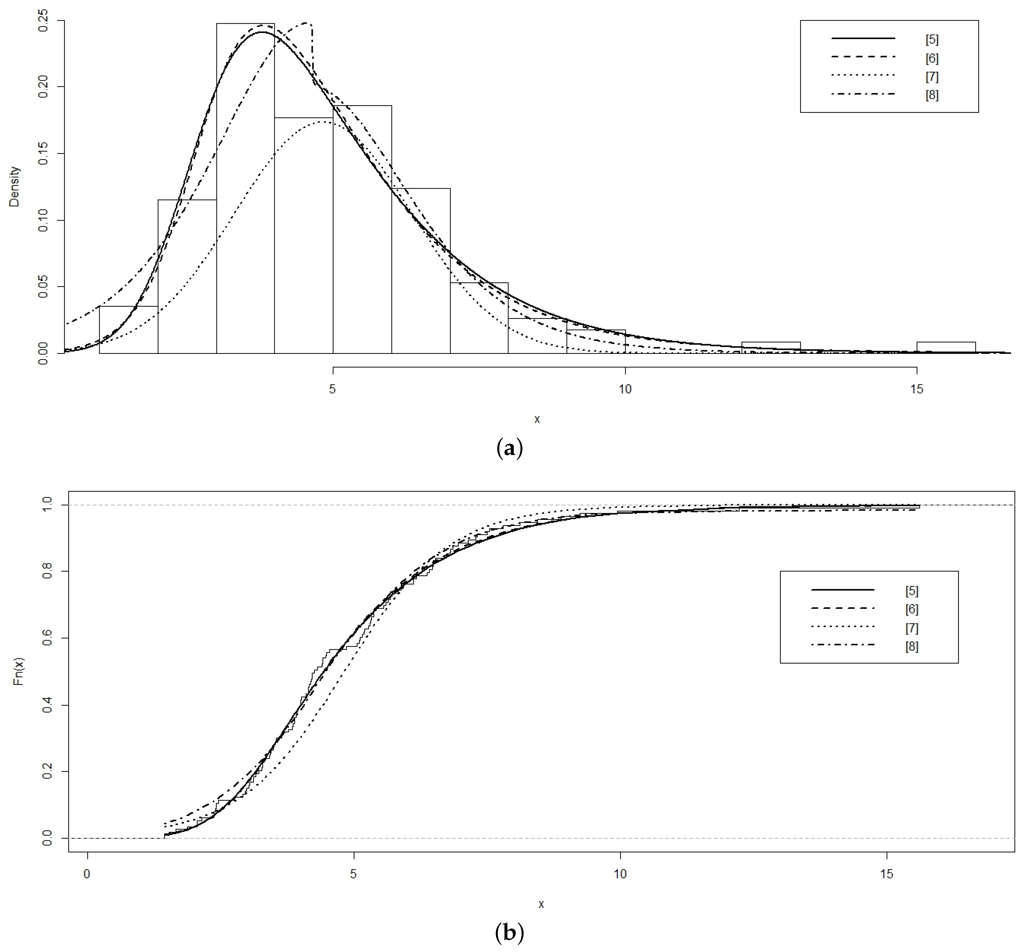
3.1. Application 1: Expenditure on Education

We use the data of total spending on public education (% of GDP- Gross Domestic Product) in various countries in 2003. These data were obtained from [15]. Expenditure on public education includes the current and capital spending by private and government agencies on educational institutions (both public and private), educational administration and subsidies to private (student/family) entities.

To adjust this data set, we modify the models by introducing a location parameter μ and a scale parameter σ by changing x to $(x-\mu )/\sigma$ everywhere in the density function divided by σ. The software R was used to calculate the estimates of the parameters through maximum likelihood method and the R function $constrOptim$ [16] was used to maximize the log-likelihood function (Appendix A). The reason for using the R function $constrOptim$ is to guarantee that the estimated parameters are consistent within their respective parametric space. The maximum likelihood estimates for the parameters of the models are given by:

• Skew Normal-GL: $\widehat{A}=-0.000227$, $\widehat{B}=-8.83\times {10}^{-14}$, $\widehat{p}=2.29$, $\widehat{\mu }=4.83$ and $\widehat{\sigma }=1.51$;
• Skew GL-Normal: $\widehat{a}=22.76$, $\widehat{b}=2.67$, $\widehat{p}=26.40$, $\widehat{c}=43.94$, $\widehat{\mu }=2.60$ and $\widehat{\sigma }=38.21$;
• Skew t-GL: $\widehat{A_1}=0.167$, $\widehat{B_1}=0.005$, $\widehat{p}=5.19$, $\widehat{v}=3.44$, $\widehat{\mu }=4.21$ and $\widehat{\sigma }=1.40$;
• Skew GL-t: $\widehat{a}=22.75$, $\widehat{b}=2.55$, $\widehat{p}=26.66$, $\widehat{v}=1968.59$, $\widehat{c}=43.92$, $\widehat{\mu }=2.60$ and $\widehat{\sigma }=38.18$.

We compare the results of our distribution with the corresponding distribution (special cases) introduced by Nadarajah and Kotz [6] (Skew Normal-Logistic, Skew Logistic-Normal, Skew t-Logistic and Skew Logistic-t distributions). The Figure 5 illustrates the fit of the distributions introduced in this paper. The Figure B1 (Appendix B) illustrates the fit of Nadarajah and Kotz [6] distributions. The Figure 6 illustrates the $pp-plot$ of all distributions. The performance of the all fitted distributions are given in

Table 1. Performance and accuracy of the distributions.

Model	AIC	BIC	AICC	KS-Test (p-Value)	MSE	MAD	MaxD
Skew GL-Normal	448.29	429.20	461.22	0.9973	0.000387	0.0153	0.0481
Skew GL-t	448.29	429.20	461.23	0.9973	0.000387	0.0153	0.0481
Skew Normal-GL	609.70	593.33	620.91	0.1549	0.003777	0.0443	0.1417
Skew t-GL	441.69	422.60	454.62	0.866	0.001086	0.0266	0.0736
Skew Logistic-Normal	452.29	438.65	461.73	0.9973	0.000387	0.0153	0.0481
Skew Logistic-t	465.02	448.66	476.23	0.9818	0.000683	0.0210	0.0588
Skew Normal-Logistic	611.70	598.06	621.14	0.1549	0.004160	0.0581	0.1449
Skew t-Logistic	450.39	434.02	461.59	0.9973	0.000389	0.0154	0.0459

. Observing the results in Table 1 we can see that, looking the p-value of the KS test, all distributions can be used to model the data. According to the accuracy, the Skew GL-Normal, Skew GL-t and Skew Logistic-Normal distributions indicated better results with similar values. However, Skew GL-Normal and Skew GL-t distributions presented smaller values of AIC, BIC and AICC compared to the Skew Logistic-Normal distribution. In contrast, Skew Normal-Logistic distribution showed the worst results followed by Skew Normal-GL distribution.

Comparing the proposed distributions in this paper with their corresponding distributions given by Nadarajah and Kotz [6], we can see that: (1) Skew GL-t and Skew Normal-GL distributions have lower values of AIC, BIC, AICC , MSE , MAD and MaxD compared to the Skew Logistic-t and Skew Normal-Logistic distributions, respectively; (2) The Skew t-Logistic gave better accuracy compared to Skew distribution t-GL (Smaller values of MSE, MAD and MaxD), however, Skew t-GL distribution indicated better performance than Skew t-Logistic distribution (Smaller values of AIC, BIC and AICC).

Thus, for this application, in general, the distributions introduced in this paper fit better the data and the Skew GL-Normal and Skew GL-t distributions are preferable to fit this data because they present better and similar results (smaller values of AIC, AICC, BIC, MSE, MAD and MaxD).

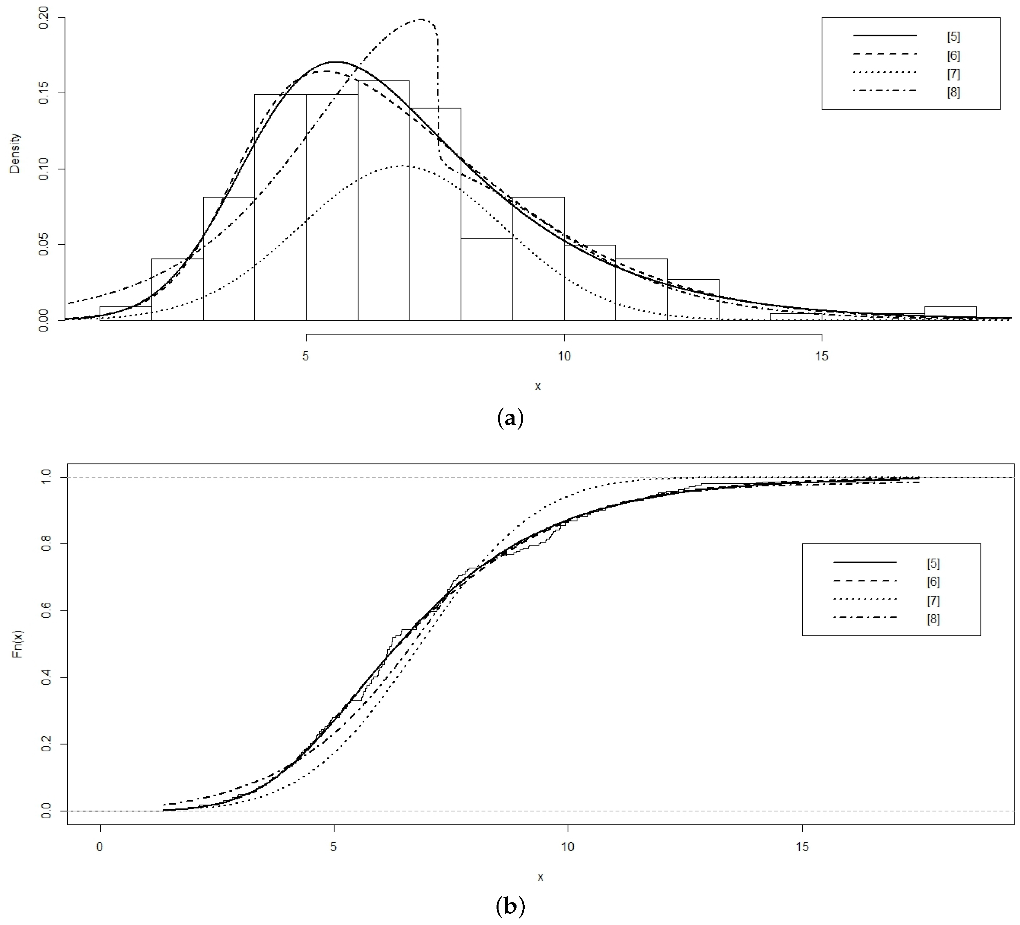
3.2. Application 2: Expenditure on Health

We use the data of total expenditure, in 2009, on health (% of GDP—Gross Domestic Product) in various countries. These data are obtained from [17]. Total health expenditure is the sum of expenses with public and private health. It covers the provision of health services (preventive and curative), family planning activities, nutrition activities and emergency aid designated for health but does not include water supply and sanitation.

Again, to adjust this data set we introduced a location parameter μ and a scale parameter σ. For the estimates of model parameters the maximum likelihood method is used. The software R was used to calculate estimates of the parameters by using the R function $constrOptim$ [16] to maximize the log-likelihood function (Appendix A). The maximum likelihood estimates for the parameters of the models are given by:

• Skew Normal-GL: $\widehat{A}=9.51\times {10}^{-8}$, $\widehat{B}=0.0005$, $\widehat{p}=7.28$, $\widehat{\mu }=6.62$ and $\widehat{\sigma }=1.99$;
• Skew GL-Normal: $\widehat{a}=0.38$, $\widehat{b}=3.30$, $\widehat{p}=0.54$, $\widehat{c}=-1.39$, $\widehat{\mu }=8.61$ and $\widehat{\sigma }=5.98$;
• Skew t-GL: $\widehat{A_1}=8.86\times {10}^{-7}$, $\widehat{B_1}=0.069$, $\widehat{p}=4.41$, $\widehat{v}=4.61$, $\widehat{\mu }=5.84$ and $\widehat{\sigma }=2.28$;
• Skew GL-t: $\widehat{a}=0.37$, $\widehat{b}=4.07$, $\widehat{p}=0.53$, $\widehat{v}=0.72$, $\widehat{c}=-4.02$, $\widehat{\mu }=8.60$ and $\widehat{\sigma }=6.78$.

We compare the results of our distribution with the corresponding distribution (special cases) introduced by Nadarajah and Kotz [6] (Skew Normal-Logistic, Skew Logistic-Normal, Skew t-Logistic and Skew Logistic-t distributions). The Figure 7 illustrates the fit of the distributions introduced in this paper. The Figure B2 (Appendix B) illustrates the fit of Nadarajah and Kotz [6] distributions. The Figure 8 illustrates the $pp-plot$ of all distributions. The performance of the all fitted distributions are included in

Table 2. Performance and accuracy of the distributions.

Model	AIC	BIC	AICC	KS-Test (p-Value)	MSE	MAD	MaxD
Skew GL-Normal	1040.04	1016.26	1050.52	0.993	0.000169	0.0104	0.0379
Skew GL-t	1038.21	1017.54	1050.42	0.9904	0.000152	0.0103	0.0378
Skew Normal-GL	1426.81	1406.42	1438.42	0.05759	0.003472	0.0497	0.1226
Skew t-GL	1048.29	1024.50	1061.76	0.9774	0.000196	0.0103	0.0402
Skew Logistic-Normal	1041.70	1024.71	1051.42	0.993	0.000211	0.0110	0.0401
Skew Logistic-t	1057.58	1037.19	1069.18	0.2235	0.001299	0.0279	0.0975
Skew Normal-Logistic	1442.35	1425.36	1452.07	0.02585	0.005780	0.0686	0.1371
Skew t-Logistic	1040.60	1019.22	1054.21	0.9774	0.000233	0.0111	0.0407

. Observing the Figure 7 we can see that the data presents a bimodal and asymmetric behavior, even if it is not very evident.

Observing the results in Table 2 we can see that, through the p-value of the KS test, only the Skew-Normal Logistic distribution could not be used to model the data. The Skew GL-t distribution had the smallest values of AIC, BIC, AICC, MSE, MAD and MaxD followed by Skew GL-Normal and Skew t-Logistics distributions. In contrast, Skew-Normal Logistic distribution showed the worst results followed by Skew Normal-GL distribution.

Comparing the distributions proposed in this paper with their corresponding distributions given by Nadarajah and Kotz [6], we can see that: (1) the Skew GL-Normal Skew GL-t and Skew Normal-GL distributions has smaller values of AIC, BIC, AICC, MSE, MAD and MaxD compared to the Skew Logistic-Normal Skew Logistic-t and Skew Normal-Logistic distributions, respectively; (2) The Skew t-Logistic distribution resulted in better performance when compared to the Skew t-GL distribution (Smaller values of AIC, BIC and AICC), however, the Skew t-GL distribution obtained better accuracy than Skew t-Logistic distribution (Smaller values of MSE, MAD and MaxD).

Again, for this application, in general, the distributions proposed in this paper fit better the data and the Skew GL-t distribution is preferred to fit this data presenting better results (smaller values of AIC, AICC, BIC, MSE, MAD and MaxD).

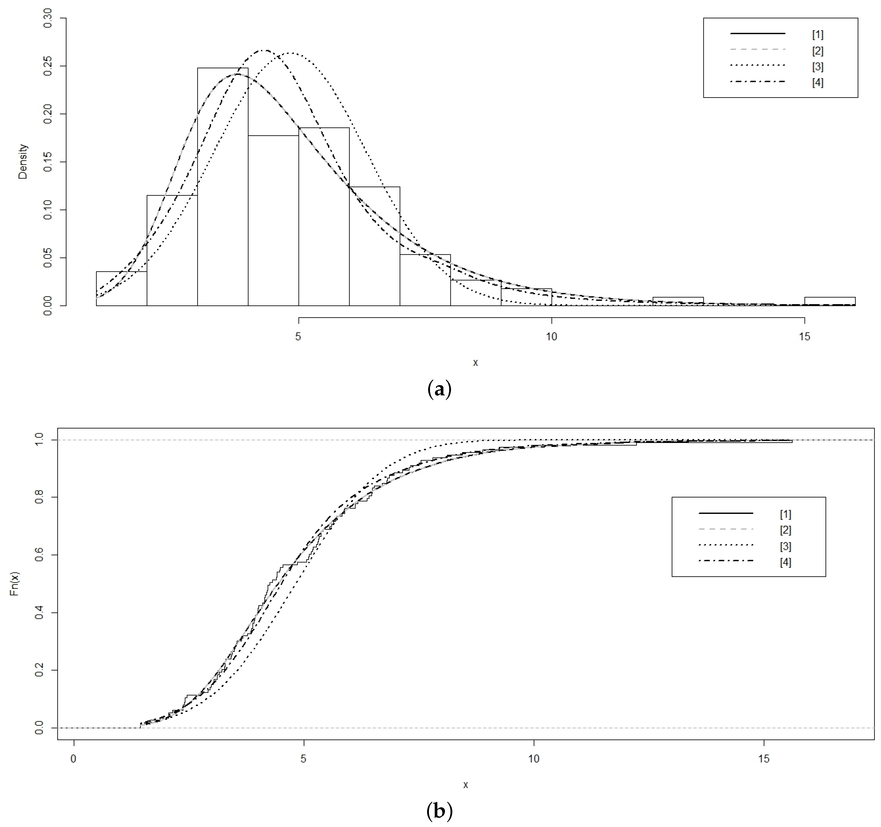
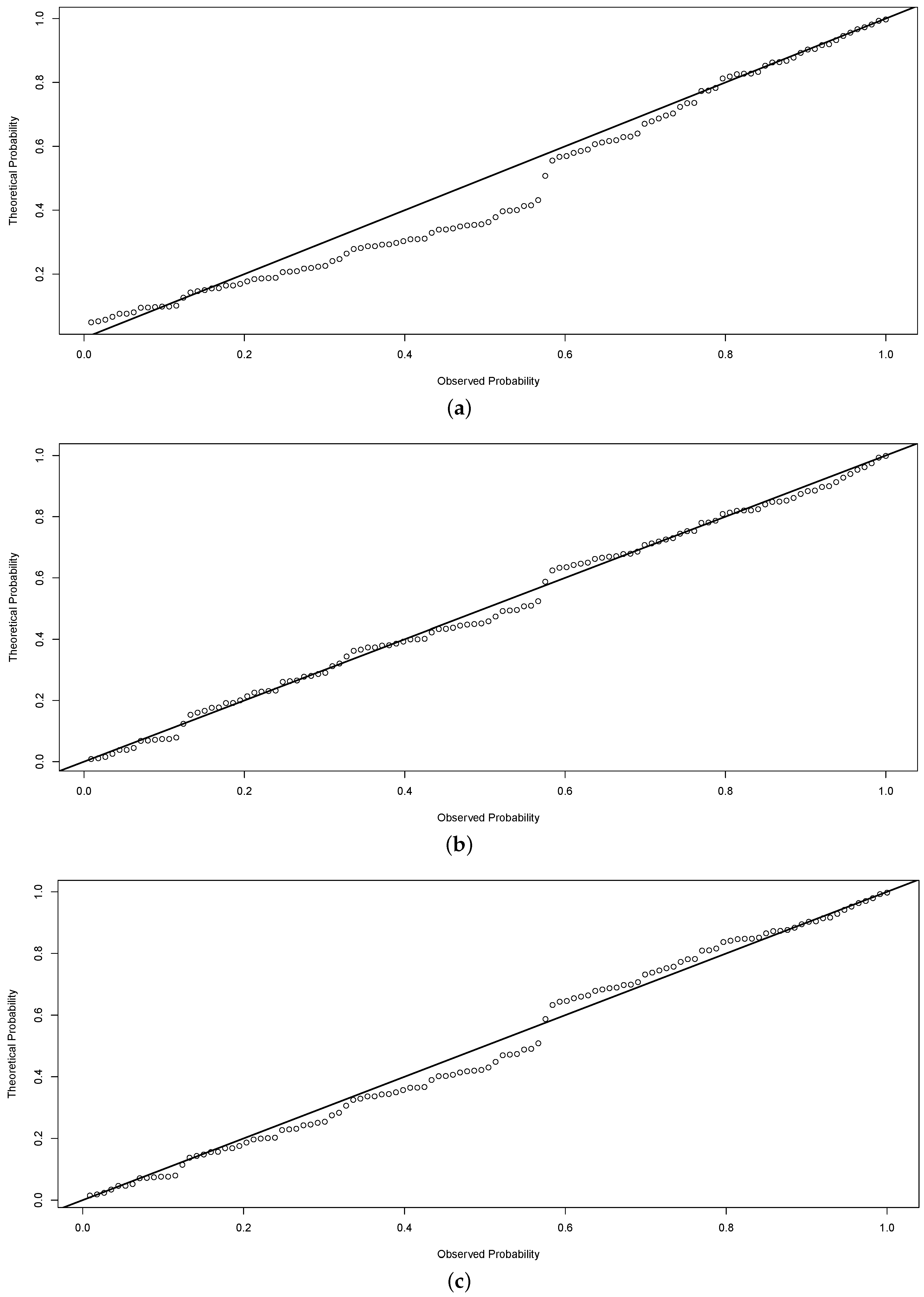
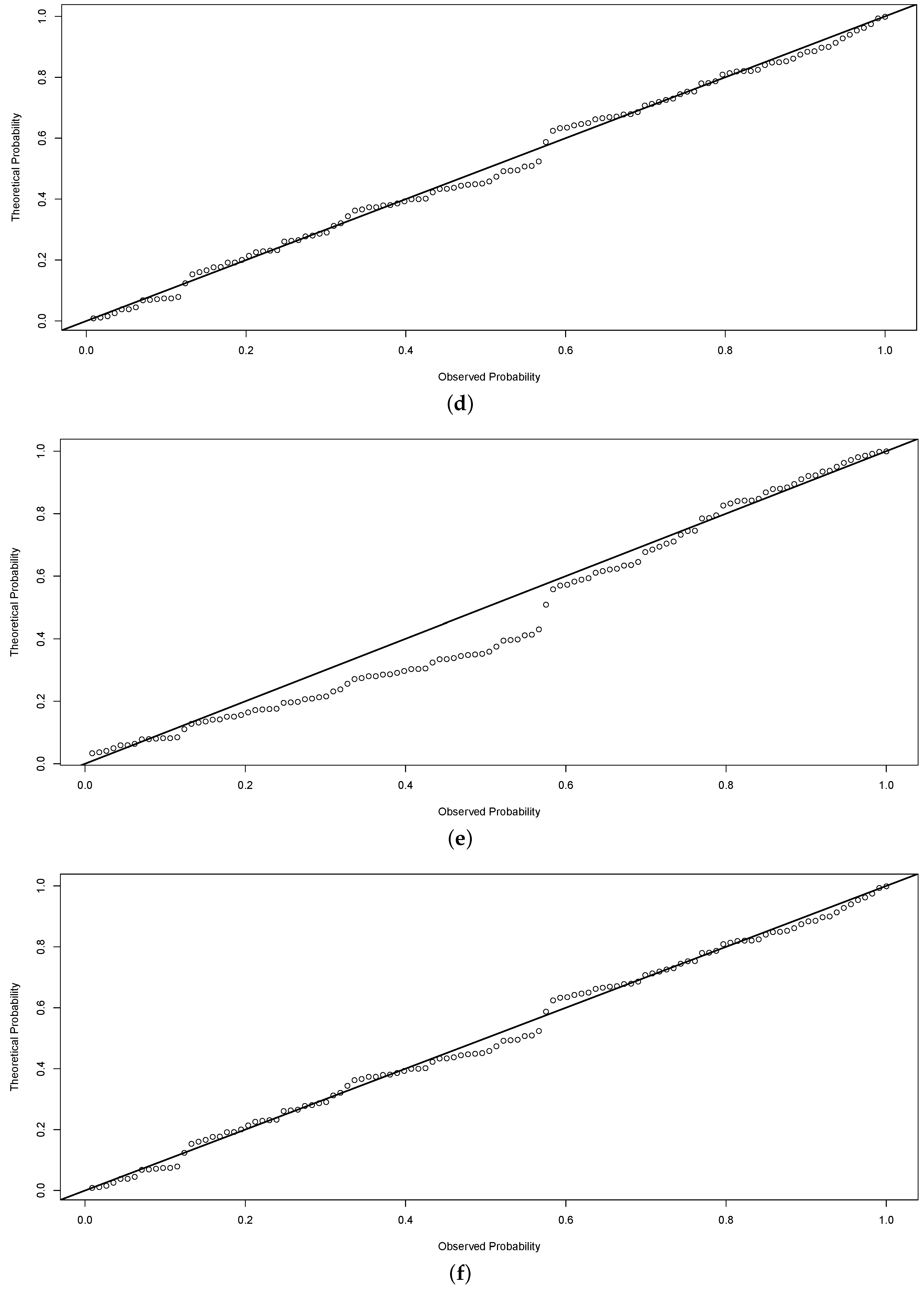
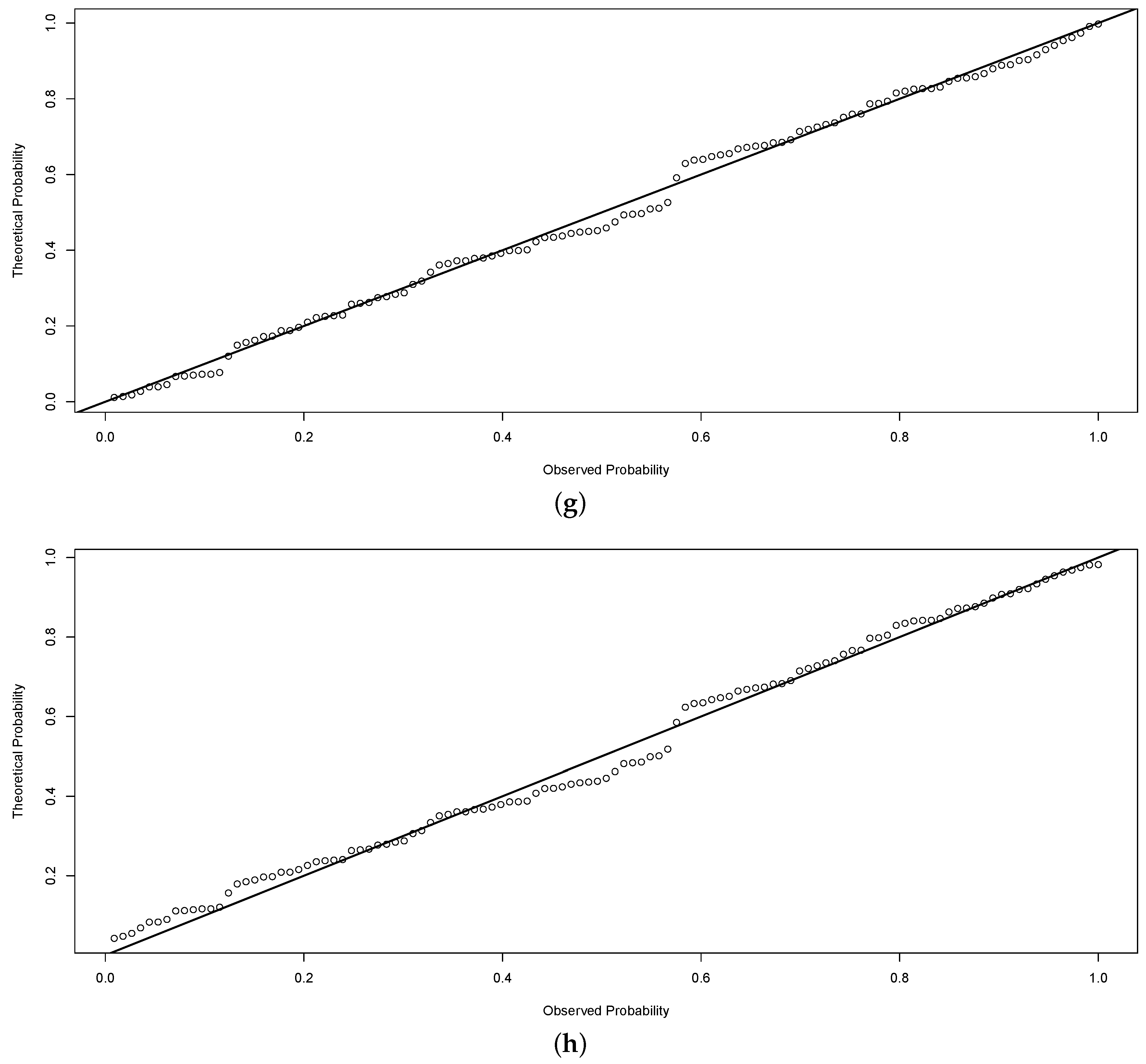
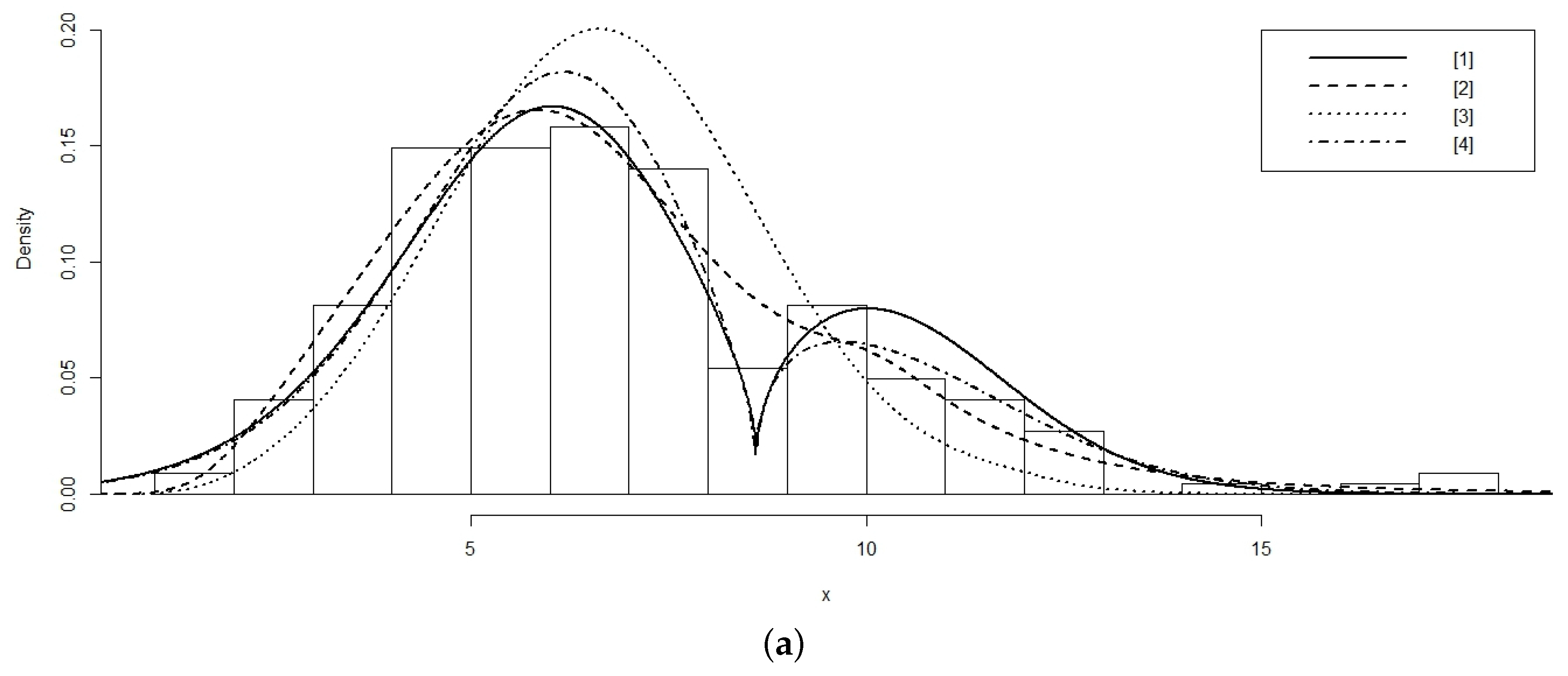
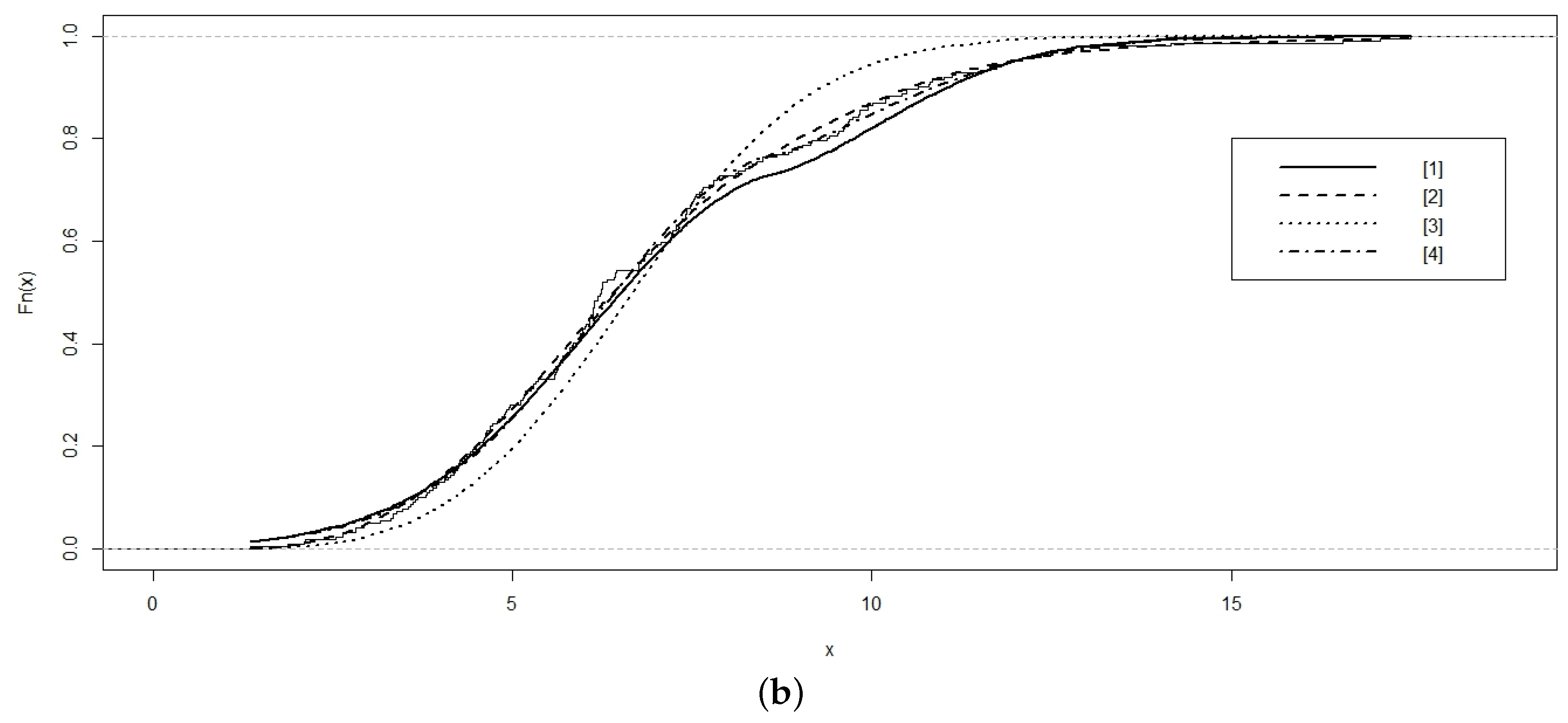
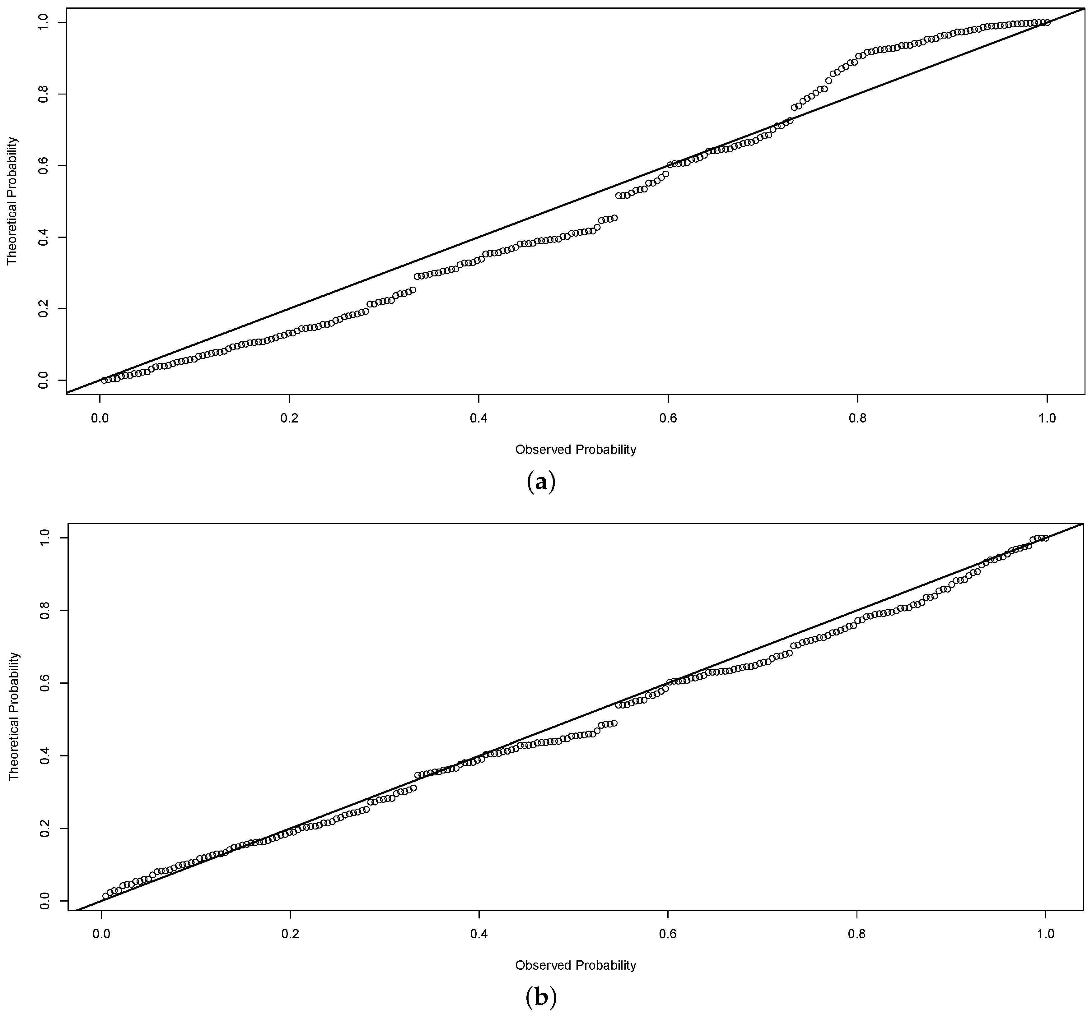
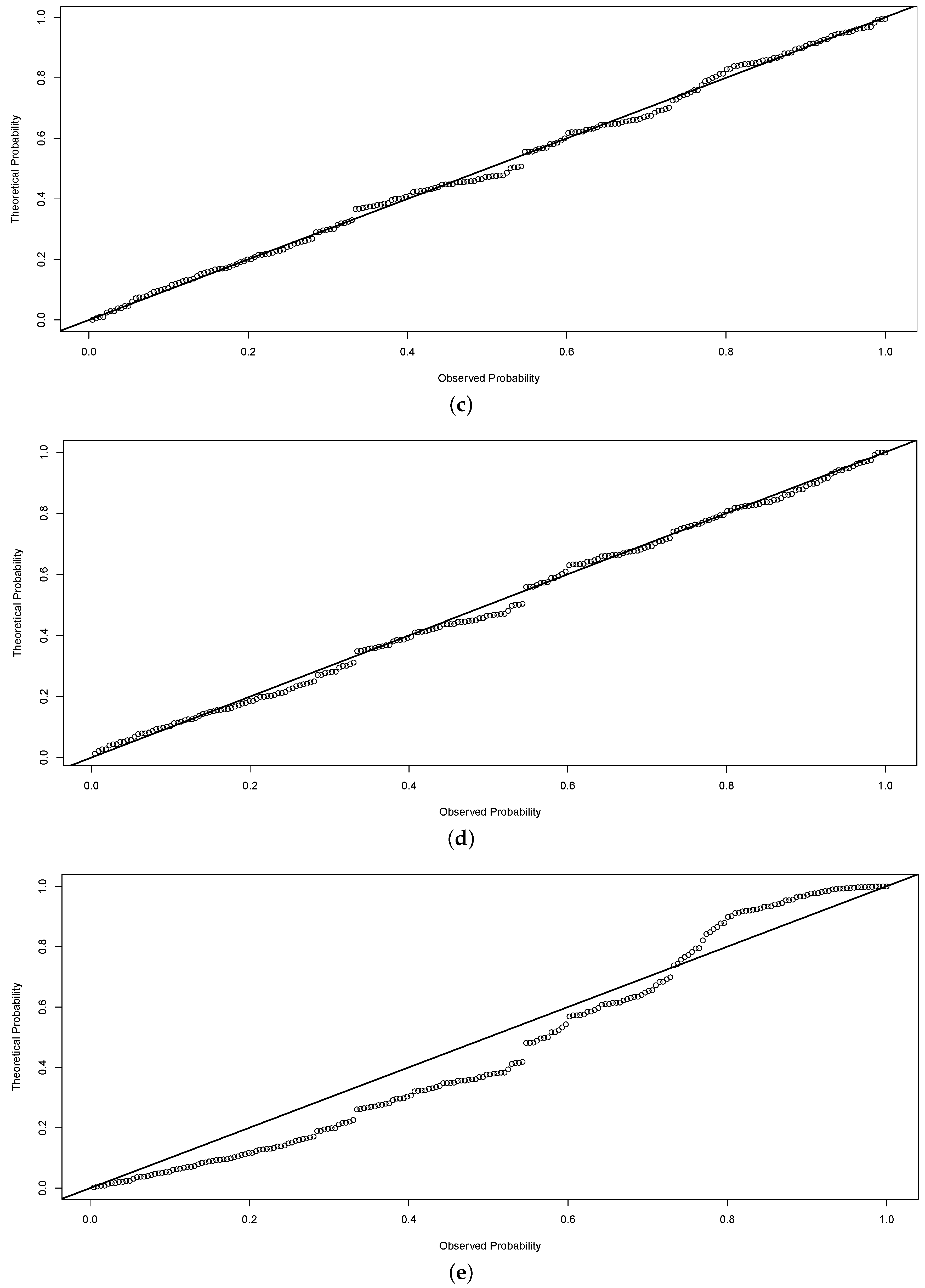
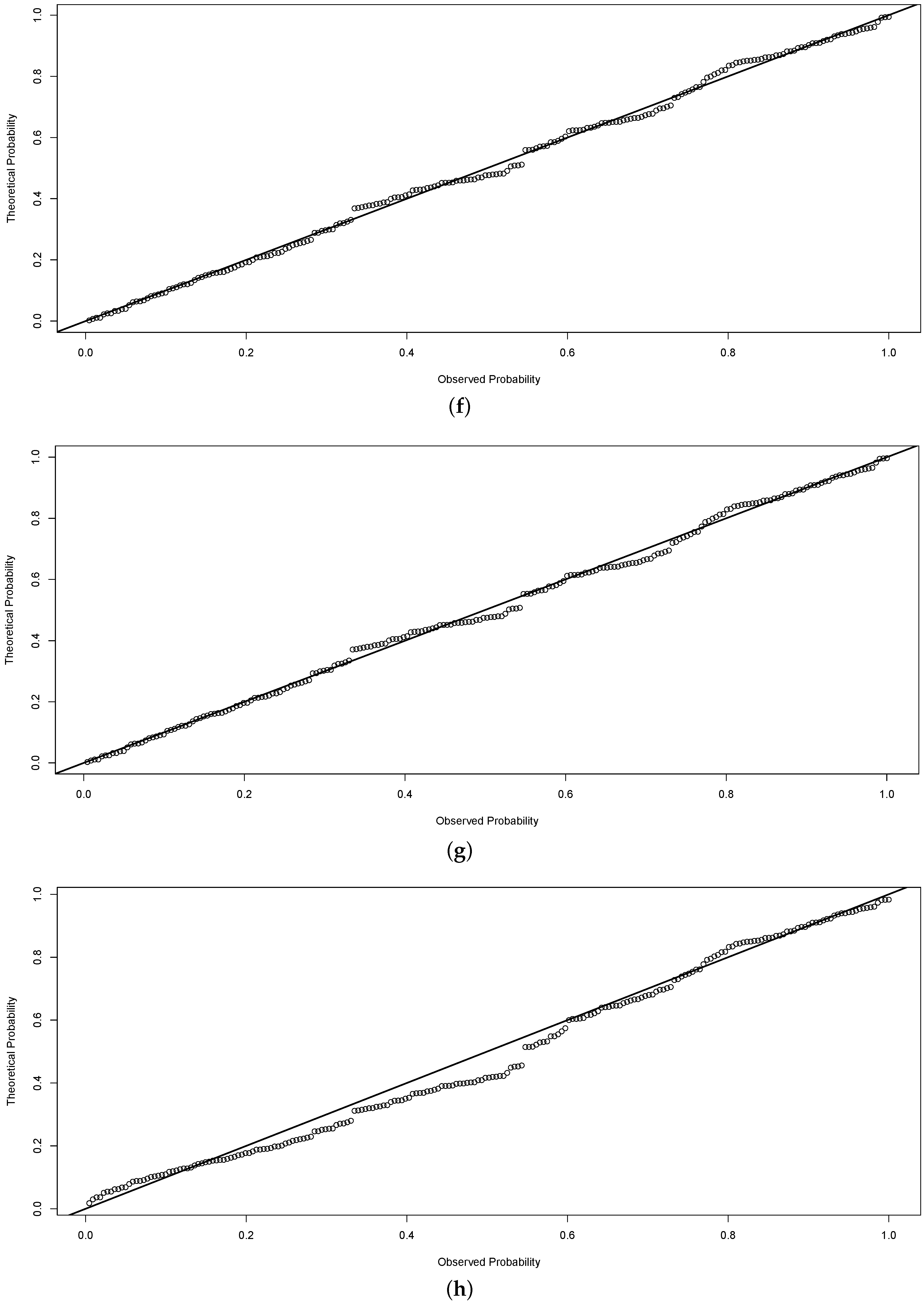
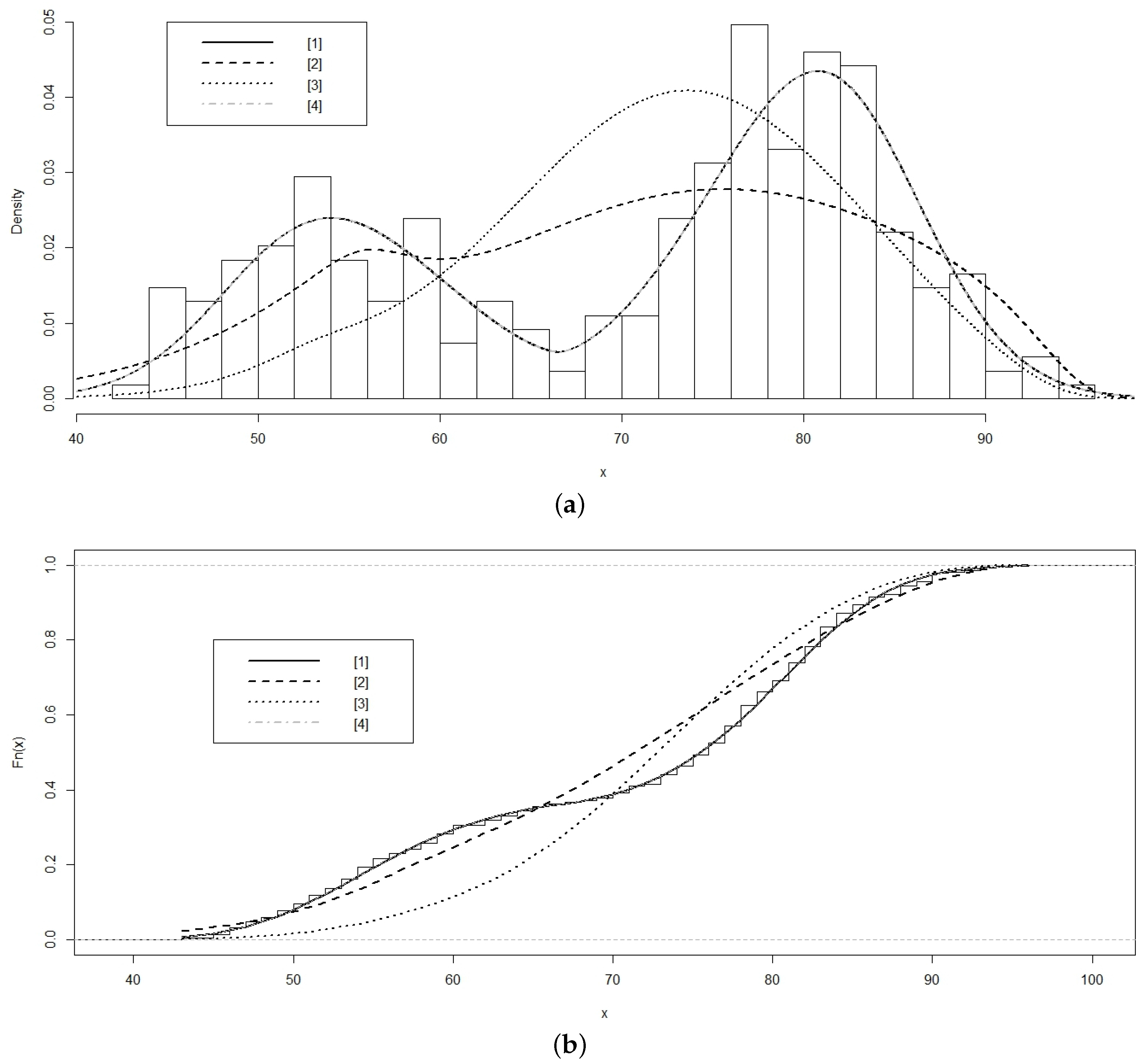
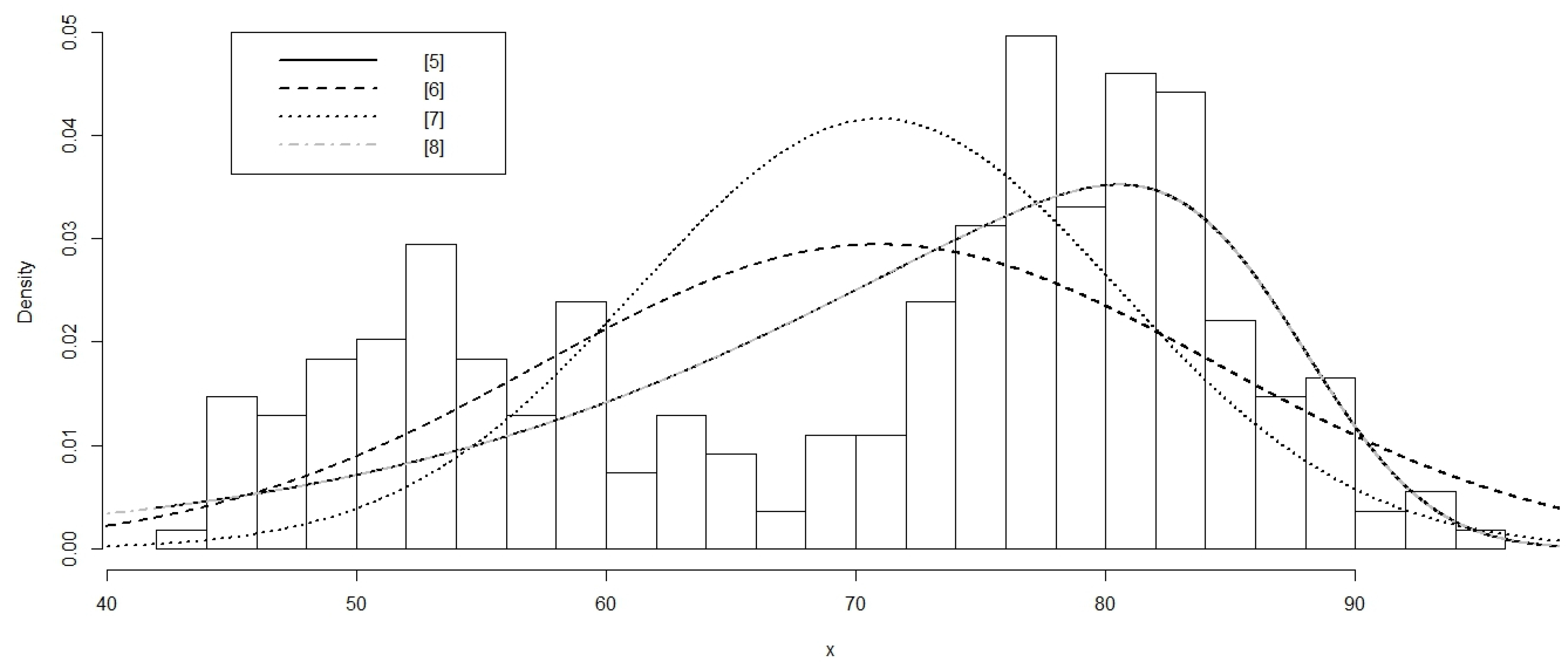
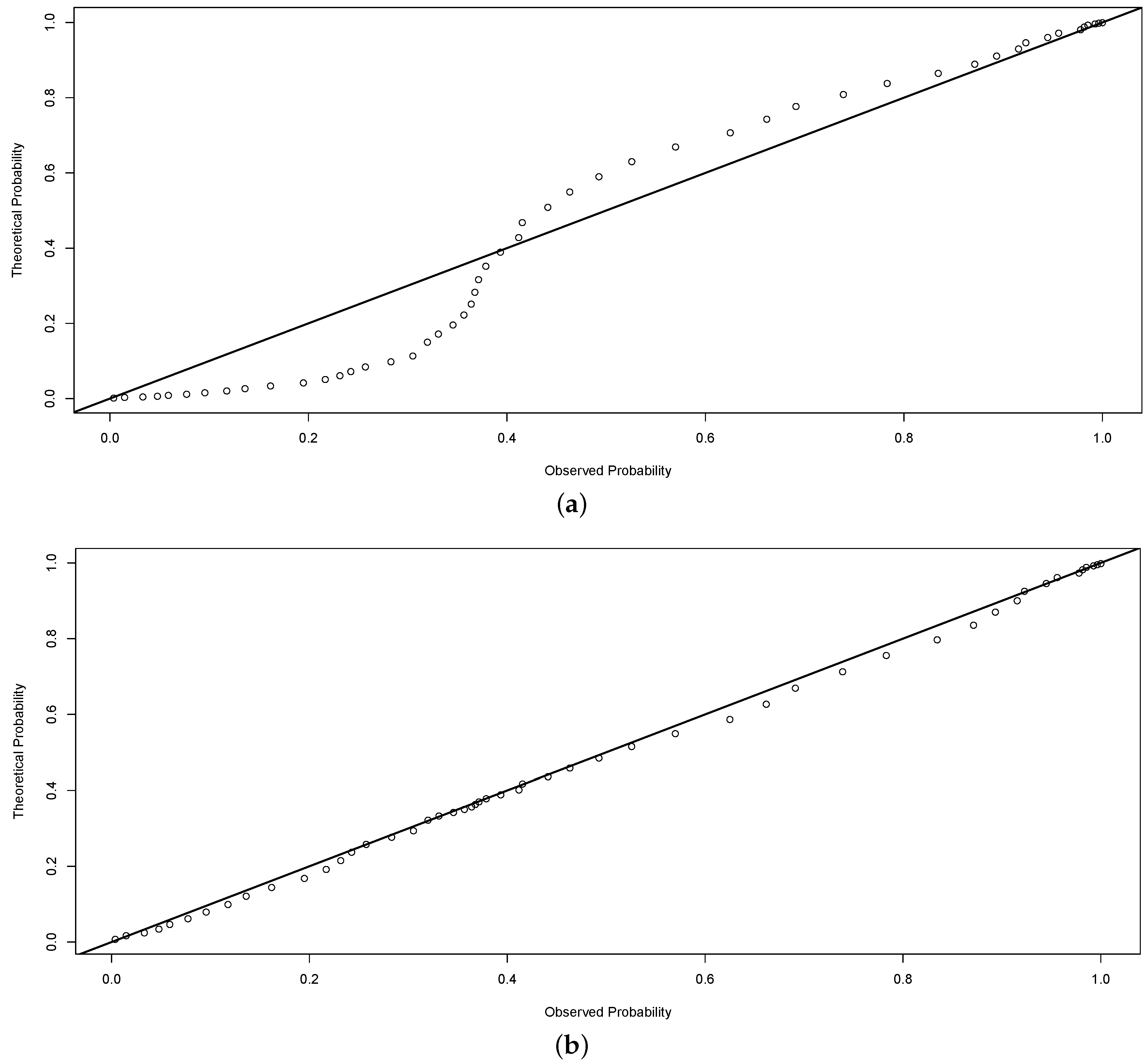
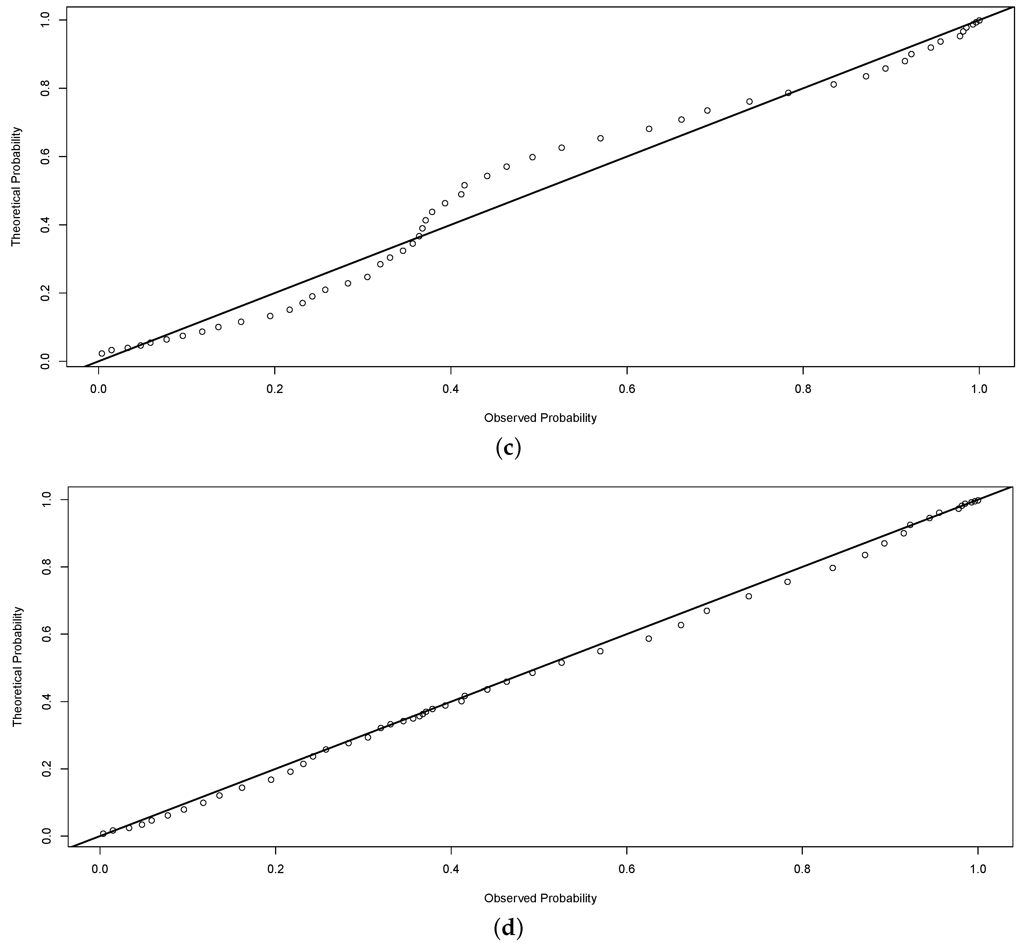
3.3. Application 3: Waiting Time between Eruptions of Old Faithful Geyser

This application shows the versatility of the Skew GL-Normal and the Skew GL-t distributions. Using data available in the free statistical software R we see the shape of bimodal distribution. Among the variables available, the waiting time between eruptions of Old Faithful Geyser in Yellow Stone National Park, Wyoming, USA was used. The data has 272 observations given in minutes.

Once more, to adjust this data set we modify the models by introducing a location parameter μ and a scale parameter σ. The software R was used to calculate the estimates of the parameters through maximum likelihood method and the R function $constrOptim$ [16] was used to maximize the log-likelihood function (Appendix A). The maximum likelihood estimates for the parameters of the models are given by:

• Skew Normal-GL: $\widehat{A}=-8.23\times {10}^{-8}$, $\widehat{B}=-0.010$, $\widehat{p}=5.94$, $\widehat{\mu }=73.59$ and $\widehat{\sigma }=9.76$;
• Skew GL-Normal: $\widehat{a}=0.42$, $\widehat{b}=1.59$, $\widehat{p}=1.57$, $\widehat{c}=0.48$, $\widehat{\mu }=66.59$ and $\widehat{\sigma }=17.31$;
• Skew t-GL: $\widehat{A_1}=-3.33\times {10}^{-8}$, $\widehat{B_1}=-0.222$, $\widehat{p}=6.37$, $\widehat{v}=10714.65$, $\widehat{\mu }=75.58$ and $\widehat{\sigma }=14.37$;
• Skew GL-t: $\widehat{a}=0.89$, $\widehat{b}=10.89$, $\widehat{p}=1.57$, $\widehat{v}=35.10$, $\widehat{c}=1.02$, $\widehat{\mu }=66.59$ and $\widehat{\sigma }=36.51$.

We now compare the results of our distribution with the corresponding distribution (special cases) introduced by Nadarajah and Kotz [6] (Skew Normal-Logistic, Skew Logistic-Normal, Skew t-Logistic and Skew Logistic-t distributions). It is interesting to note that, when we try to adjust the distributions given by Nadarajah and Kotz [6] to the data, which have a marked bimodal behavior, we had numerical problems when trying to calculate their cumulative distribution functions, which did not happen with our distributions. Thus, it was not possible to calculate the p-value of the KS test, MSE, MAD and MaxD for the Skew Normal-Logistic, Skew Logistic-Normal, Skew t-Logistic and Skew Logistic-t distributions.

The Figure 9 illustrates the fit of the distributions introduced in this paper. The Figure 10 illustrates the fit of the density function of the distributions introduced by Nadarajah and Kotz [6]. The Figure 11 illustrates the $pp-plot$ of our distributions. The performance of the all fitted distributions are given in

Table 3. Performance and accuracy of the distributions.

Model	AIC	BIC	AICC	KS-Test (p-Value)	MSE	MAD	MaxD
Skew GL-Normal	2055.26	2033.63	2066.95	0.7344	0.000439	0.0171	0.0378
Skew GL-t	2053.27	2028.02	2066.84	0.7344	0.000439	0.0171	0.0378
Skew Normal-GL	3454.74	3433.11	3466.43	<0.0001	0.009393	0.0805	0.1915
Skew t-GL	2120.98	2095.74	2134.55	0.01705	0.002896	0.0448	0.1077
Skew Logistic-Normal	2149.71	2131.68	2159.49	-	-	-	-
Skew Logistic-t	2147.71	2126.08	2159.40	-	-	-	-
Skew Normal-Logistic	3494.18	3476.15	3503.95	-	-	-	-
Skew t-Logistic	2178.58	2156.95	2190.26	-	-	-	-

. Observing the results of the Table 3 we can see that, only the Skew GL-Normal and Skew GL-t distributions adjusted well to the data with similar accuracies. However, observing the AIC, BIC and AICC values, the Skew GL-t distribution had a slightly better result. In contrast, Skew Normal-GL and Skew t-GL distributions, even having no numerical problems, are not indicated to model these data showing poor results. Finally, the Skew Logistic-Normal Skew Logistic-t, Skew Normal-Logistic and Skew t-Logistic distributions presented numerical problems when calculating the cumulative distribution functions, showing that they are not flexible enough to model bimodal data. So, for this application, the Skew GL-t distribution is preferred to fit this data presenting better results (smaller values of AIC, AICC, BIC, MSE, MAD and MaxD).

From the results of Section 3.1, Section 3.2 and Section 3.3, we can see that: (1) in general, our distributions adjusted the data better than the distributions given by Nadarajah and Kotz [6]; (2) The Skew GL-Normal, Skew GL-t, Skew t-GL and Skew Normal-GL distributions can be used to model symmetrical and asymmetrical unimodal data; (3) Skew GL-t and Skew GL-Normal distributions can be used to adjust bimodal symmetrical and asymmetrical data, showing high flexibility which is not common in the literature on probability distributions, and this can be very important in practical applications; (4) For application 1, the Skew GL-Normal and Skew GL-t distributions are preferable to fit this data because they present better and similar results (smaller values of AIC, AICC, BIC, MSE, MAD and MaxD), and, for applications 2 and 3, the Skew GL-t distribution is preferred to fit this data presenting better results. Finally, the distributions introduced in this paper are robust to numerical computation.

4. Conclusions

In this paper, we proposed new skew probability density functions using the Azzalini’s formula $2f\left(x\right)G\left(cx\right)$, where f is a symmetric density about zero, and G is a distribution function of a symmetric density about zero. The expressions for f and G are taken from normal, student-t and generalized logistic distributions. We derived expressions for the n-th moments in terms of the H and Meijer G functions [12].

We apply new distributions to three data sets. One application for unimodal data is provided for total expenditure on education in various countries in 2003. Two applications of bimodal data are given for the total expenditure on health in various countries in 2009 and waiting time between eruptions of the Old Faithful Geyser. We conclude that:

• In general, the distributions introduced in this paper fit better the data when compared with the Skew Logistic-Normal, Skew Logistic-t, Skew Normal-Logistic and Skew t-Logistic distributions, introduced by Nadarajah and Kotz [6];
• The Skew GL-Normal, Skew GL-t, Skew Normal-GL and Skew t-GL distributions can be used to model symmetrical and asymmetrical unimodal data;
• The Skew GL-Normal and Skew GL-t distributions can be used to adjust bimodal symmetrical and asymmetrical data, offering good fits, showing a high flexibility which is not common in the literature on probability distributions, and this can be very important in practical applications;
• For application 1, the Skew GL-Normal and Skew GL-t distributions are preferable to fit this data because they present better and similar results (smaller values of AIC, AICC, BIC, MSE, MAD and MaxD), and, for applications 2 and 3, the Skew GL-t distribution is preferred to fit this data presenting better results;
• The distributions proposed in this paper apply to all applications without presenting numerical problems, unlike the proposed distributions by Nadarajah and Kotz [6] which had serious numerical problems to adjust bimodal data. (Section 3.3).

Thus, the proposed distributions in this paper are flexible to adjust symmetric and asymmetric data, with unimodal and bimodal behavior, and are robust to numerical computation in practical applications.

References

1. Abtahi, A.; Behboodian, J.; Shafari, M.A. General class of univariate skew distributions considering Stein’s lemma and infinite divisibility. Metrika 2010, 75, 193–206. [Google Scholar] [CrossRef]
2. Rathie, P.N.; Coutinho, M. A new skew generalized logistic distribution and approximations to skew normal distribution. Aligarh J. Stat. 2011, 31, 1–12. [Google Scholar]
3. Rathie, P.N.; Swamee, P.K.; Matos, G.G.; Coutinho, M.; Carrijo, T.B. H-function and statistical distributions. Ganita 2008, 59, 23–37. [Google Scholar]
4. Rathie, P.N.; Swamee, P.K. On a New Invertible Generalized Logistic Distribution Approximation to Normal Distribution; Technical Research Report No. 07/2006; Department of Statistics, University of Brasilia: Brasilia, Brazil, 2006. [Google Scholar]
5. Gupta, R.D.; Kundu, D. Generalized logistic distributions. J. Appl. Stat. Sci. 2010, 18, 51–66. [Google Scholar]
6. Nadarajah, S.; Kotz, S. Skew distributions generated from different families. Acta Appl. Math. 2006, 91, 1–37. [Google Scholar] [CrossRef]
7. Swamee, P.K.; Rathie, P.N. Invertible alternatives to normal and lognormal distributions. J. Hydrol. Eng. ASCE 2007, 12, 218–221. [Google Scholar] [CrossRef]
8. Rathie, P.N. Normal Distribution, Univariate; Springer: Berlin, Germany, 2011; pp. 1012–1013. [Google Scholar]
9. Azzalini, A. A class of distributions which includes the normal ones. Scand. J. Stat. 1985, 12, 171–178. [Google Scholar]
10. Luke, Y.L. The Special Functions and Their Approximations; Academic Press: New York, NY, USA, 1969. [Google Scholar]
11. Springer, M.D. Algebra of Random Variables; John Wiley: New York, NY, USA, 1979. [Google Scholar]
12. Mathai, A.M.; Saxena, R.K.; Haubold, H.J. The H-Function: Theory and Applications; Springer: New York, NY, USA, 2010. [Google Scholar]
13. Gradshteyn, I.S.; Ryzhik, I.M. Table of Integrals, Series and Products; Academic Press: San Diego, CA, USA, 2000. [Google Scholar]
14. Prudnikov, A.P.; Brychkov, Y.A.; Marichev, O.I. Integrals and Series; Breach Science: Amsterdam, The Netherlands, 1986. [Google Scholar]
15. The World Bank: Working for a World Free of Poverty. Government expenditure on education as % of GDP (%). Available online: http://data.worldbank.org/indicator/SE.XPD.TOTL.GD.ZS (accessed on 1 February 2016).
16. R Core Team. R: A Language and Environment for Statistical Computing; R Foundation for Statistical Computing: Vienna, Austria, 2015; Available online: http://www.R-project.org/ (accessed on 1 February 2016).
17. The World Bank: Working for a World Free of Poverty. Health expenditure, total (% of GDP). Available online: http://data.worldbank.org/indicator/SH.XPD.TOTL.ZS (accessed on 1 February 2016).
Figure 1. The skew normal-generalized logistic distribution (Skew Normal-GL) using the following parameter values: [1] A = 6 , B = 10.8 and p = 2 ; [2] A = 0 , B = 0 and p = 3 ; [3] A = - 6 , B = - 10.8 and p = 2 .
Axioms 05 00010 g001
Figure 2. The Skew GL-Normal distribution using the following parameter values: [1] a = 1.59 , b = 0.0727 , p = 1.962 and c = 10 ; [2] a = 0.3 , b = 0.7 , p = 0.4 and c = 0.6 ; [3] a = 1.59 , b = 0.0727 , p = 1.962 and c = 0 ; [4] a = 1.59 , b = 0.0727 , p = 1.962 and c = - 10 .
Axioms 05 00010 g002
Figure 3. The Skew t-GL distribution using the following parameter values: [1] A 1 = 6 , B 1 = 10.8 , v = 2 and p = 2 ; [2] A 1 = 0 , B 1 = 0 , v = 4 and p = 3 ; [3] A 1 = - 6 , B 1 = - 10.8 , v = 2 and p = 2 .
Axioms 05 00010 g003
Figure 4. The Skew GL-t distribution using the following parameter values: [1] a = 1.59 , b = 0.0727 , p = 1.962 , v = 2 and c = 10 ; [2] a = 0.3 , b = 0.7 , p = 0.4 , v = 3 and c = 0.6 ; [3] a = 1.59 , b = 0.0727 , p = 1.962 , v = 3 and c = 0 ; [4] a = 1.59 , b = 0.0727 , p = 1.962 , v = 2 and c = - 10 .
Axioms 05 00010 g004
Figure 5. Education data - Fitted distributions. [1] Skew GL-Normal distribution; [2] Skew GL-t distribution; [3] Skew Normal-GL distribution; [4] Skew t-GL distribution. (a) Probability density function; (b) Cumulative distribution.
Axioms 05 00010 g005
Figure 6. Education data - PP-Plot. (a) Skew Normal-GL; (b) Skew GL-Normal; (c) Skew t-GL; (d) Skew GL-t; (e) Skew Normal-Logistic; (f) Skew Logistic-Normal; (g) Skew t-Logistic; (h) Skew Logistic-t.
Axioms 05 00010 g006aAxioms 05 00010 g006bAxioms 05 00010 g006c
Figure 7. Health data - Fitted distributions. [1] Skew GL-Normal distribution; [2] Skew GL-t distribution; [3] Skew Normal-GL distribution; [4] Skew t-GL distribution. (a) Probability density function; (b) Cumulative distribution.
Axioms 05 00010 g007aAxioms 05 00010 g007b
Figure 8. Health data - PP-Plot. (a) Skew Normal-GL; (b) Skew GL-Normal; (c) Skew t-GL; (d) Skew GL-t; (e) Skew Normal-Logistic; (f) Skew Logistic-Normal; (g) Skew t-Logistic; (h) Skew Logistic-t.
Axioms 05 00010 g008aAxioms 05 00010 g008bAxioms 05 00010 g008c
Figure 9. Faithful data - Fitted distributions. [1] Skew GL-Normal distribution; [2] Skew GL-t distribution; [3] Skew Normal-GL distribution; [4] Skew t-GL distribution. (a) Probability density function; (b) Cumulative distribution.
Axioms 05 00010 g009
Figure 10. Faithful data - Fitted Nadarajah and Kotz [6] distributions. [5] Skew Logistic-Normal distribution; [6] Skew Logistic-t distribution; [7] Skew Normal-Logistic distribution; [8] Skew t-Logistic distribution.
Axioms 05 00010 g010
Figure 11. Faithful data - PP-Plot. (a) Skew Normal-GL; (b) Skew GL-Normal; (c) Skew t-GL; (d) Skew GL-t.
Axioms 05 00010 g011aAxioms 05 00010 g011b