
An Improved Evaluation Methodology for Mining Association Rules


1
Contemporary Business and Trade Research Center, Zhejiang Gongshang University, Hangzhou 310018, China
2
School of Management and E-business, Zhejiang Gongshang University, Hangzhou 310018, China
3
Academy of Zhejiang Culture Industry Innovation & Development, Zhejiang Gongshang University, Hangzhou 310018, China
4
School of Foreign Languages, Zhejiang Gongshang University, Hangzhou 310018, China
5
School of Business Administration, Zhejiang Gongshang University, Hangzhou 310018, China
*
Author to whom correspondence should be addressed.
Axioms 2022, 11(1), 17; https://doi.org/10.3390/axioms11010017
Submission received: 5 December 2021
/
Revised: 29 December 2021
/
Accepted: 30 December 2021
/
Published: 31 December 2021
(This article belongs to the Section Mathematical Analysis)
Abstract
:At present, association rules have been widely used in prediction, personalized recommendation, risk analysis and other fields. However, it has been pointed out that the traditional framework to evaluate association rules, based on Support and Confidence as measures of importance and accuracy, has several drawbacks. Some papers presented several new evaluation methods; the most typical methods are Lift, Improvement, Validity, Conviction, Chi-square analysis, etc. Here, this paper first analyzes the advantages and disadvantages of common measurement indicators of association rules and then puts forward four new measure indicators (i.e., Bi-support, Bi-lift, Bi-improvement, and Bi-confidence) based on the analysis. At last, this paper proposes a novel Bi-directional interestingness measure framework to improve the traditional one. In conclusion, the bi-directional interestingness measure framework (Bi-support and Bi-confidence framework) is superior to the traditional ones in the aspects of the objective criterion, comprehensive definition, and practical application.
1. Introduction
Nowadays, the amount of data stored in databases has grown in an impressive way. Thus, one of the main motivations for data storage is to obtain access to data so as to further analyze them and to obtain valuable and useful information from the data. As data mining methodology and technology have received extensive attention, association rules mining, as a vital subject in the domain of data mining and knowledge discovery, is now widely used in the field of electronic commerce [1,2,3,4,5]. Apriori algorithm can mine a host of association rules; however, only a few rules could be laid down and implemented by makers on account of limited resources [6,7]. Consequently, the evaluation methodology for mining association rules is of great significance in both theory design and practical application.
In recent years, quite a few results have been achieved in the study on the interestingness measure of association rules [8,9,10,11]. Tseng et al. [10] put forward incremental maintenance of generalized association rules under taxonomy evolution. Chen [12] used data envelopment analysis (DEA) as a post-processing approach. After the rules had been discovered from the association rule mining algorithms, DEA was applied to the use of ranking those discovered rules based on the specified criteria. Toloo et al. [13] proposed a new integrated DEA model, which was able to find the most efficient association rule only by solving one mixed integer linear programming (MILP). Objective interestingness mainly considers statistical significance features of objective data, including Support, Confidence and Lift, which are classic, as well as Validity, Conviction, Improvement, and Chi-square analysis, which are relatively new [14]. Some scholars came up with some methods to generate both frequent and infrequent patterns by using a multi-objective genetic algorithm [15,16]. It is the common goal of researchers to mine association rules that can reflect users’ interests truly and effectively.
Firstly, the traditional methods of association rule mining generate excessive association rules that include many invalids or even erroneous association rules. Secondly, with the current surge in online transactions, data on online transactions and user evaluation are extremely sparse. Thirdly, a combination of explosion problems may occur when the Support and Confidence thresholds are low, while some new knowledge of user interest will be filtered out because of data sparseness when the Support and Confidence thresholds are high. Lastly, the traditional Support and Confidence frameworks can no longer measure association rules in an effective way.
The main contributions of this paper are summarized as follows:
- (1)
- This paper firstly expounds several aspects of association rules and then makes a summary of relevant research results on the objective interestingness measure of association rules. At the same time, we find that all have some defects and problems by discussing and comparing the various measurement methods of association rules.
- (2)
- Then, we proposed four more effective measurement methods of association rules (Bi-support, Bi-lift, Bi-improvement, and Bi-confidence) based on the improvement of some methods. The Bi-confidence method makes an adjustment to the non-occurrence possibility of an antecedent based on the Confidence.
- (3)
- Through the experimental analysis, we propose a novel measure framework (Bi-support and Bi-confidence framework) to improve the traditional one.
In Section 2, a review of related work is provided. In Section 3, interestingness measure indicators for association rules are described. In Section 4, four more effective measurement methods of association rules (Bi-support, Bi-lift, Bi-improvement, Bi-confidence) are proposed. In Section 5, we propose a novel Bi-directional interestingness framework to improve the traditional one through the experimental analysis. Finally, we draw conclusions in Section 6.
2. A Review of Relevant Research on Association Rules
This paper describes the research status of association rules from three parts: the algorithm, the application, and the evaluation method of association rules.
2.1. Algorithm of Association Rules
The Apriori algorithm is the earliest proposed classical association rules mining algorithm, whose implementation process is relatively simple. However, the database needs to be scanned many times, leading to a large I/O load and low algorithm execution efficiency. In order to solve the defects of Apriori, Pal and Kumar [17] proposed a distributed frequent itemset generation and association rule mining algorithm based on the MapReduce programming model. This scheme uses integrated distributed technology to generate frequent itemsets and mine association rules. Rules are mined in a distributed way, after which weights are assigned to the data subsets and association rules, and the association rules generated in a distributed way are mixed by the weighting method. This method solves the problem of multifarious operation when the data are large. Huo et al. [18] proposed an improved FP-tree algorithm to solve the defects of the Apriori algorithm. They set up the FP-tree-based (initial-FP-tree and new-FP-tree) structures to maintain fuzzy frequent itemsets in the original database and newly inserted transactions, respectively. The incremental mining strategy of fuzzy frequent itemsets is implemented by breathing priority traversal of the initial-FP-tree and new-FP-tree. This method has advantages in execution time. When the minimum Support threshold is low, the memory cost of this algorithm is lower than that of existing algorithms. In order to improve the speed and accuracy of association rule mining, Liu et al. [19] proposed a parallel FP growth method called SSPFP on the basis of Spark Streaming, which can mine frequent itemsets and association rules in real-time Streaming data in parallel.
2.2. Application of Association Rules
Association rules are applied in various fields, mainly focusing on prediction, recommendation, cause analysis, and so on. Rafiqul et al. [20] used association rules to identify fraudulent behavior of policyholders, predict bad behavior of policyholders, and help insurance companies improve business strategies and overcome fraudulent claims. For the application of association rules in the recommendation domain, Yang et al. [21] proposed a recommendation algorithm based on temporal association rules, which could discover potential interests of users by using historical behavior data without domain knowledge. Moreover, a personalized hybrid recommendation system, TP-HR, based on time-aware CF and temporal association rules was proposed, which was used to track dynamic changes in user preferences. For feature analysis, Sanmiquel et al. [22] used association rules to analyze occupational accidents in the mining industry and identified the 20 most important factors leading to accidents.
2.3. Evaluation Method of Association Rules
The most widely accepted evaluation indexes of association rules are Support and Confidence. Meanwhile, Lift, Validity, Conviction, Influence, and other indicators have been gradually applied in various studies related to association rules. However, with the explosive growth of data volume and data types, these indicators are faced with problems, such as a large amount of computation and sparse data. One solution is to innovate new algorithms to improve operational efficiency. For example, Zhang et al. [23] proposed a multi-objective optimization algorithm to mine frequent itemsets of high-dimensional data. The other is to improve the evaluation method of association rules. For example, Lift and Improvement evaluation methods are optimized, and the concepts of new-lift and new-improvement are proposed in this paper.
2.4. Evaluation Method and Framework of Association Rules
Most association rule mining algorithms will generate invalid or even wrong association rules. How to identify and remove these association rules is one of the research hotspots. Song et al. [24] proposed predictability-based collective class association rule mining based on cross-validation with a new rule evaluation step. This method could remove redundant association rules and retain most of the high-value association rules. Among all kinds of entropy-based measurements, the important measures to evaluate association rules are joint entropy, conditional entropy, mutual information, cross-entropy, and equilibrium cross-entropy. Park et al. [25] proposed symmetrically balanced cross-entropy by considering the advantages of a symmetric J measure and balanced cross-entropy in association rule evaluation. Shaharani et al. [26] presented a systematic evaluation of the rules of association identified on the basis of frequent, closed, and maximum detailed exploration algorithms by combining general measures of data mining and statistical interest and described the appropriate sequence of usage. This method can also remove redundant association rules.
3. Review on Interestingness Measure Indicators for Association Rules
Let , . indicates itemsets, and . Firstly, we suppose formal description of association rules is as follows:
Rules should meet a certain Support threshold, (min sup), and Confidence threshold, ().
Data in Table 1 are produced by data extraction and transformation from shopping mall receipts. Each line (a tuple) is shopping list data (shopping receipts); “1” refers to the list containing this item, while “0” means the opposite.
3.1. Support and Confidence
Support [27] is the percentage of transactions where the rule holds. Support can be used to assess the usefulness of association rules. When the frequencies of A and B occurring simultaneously are equal to or higher than the set Support threshold, itemsets (A, B) as a frequent pattern. The formula is as follows:
where is the number of records that A and B appear together, and is the total record number of transactions in data sets.
Firstly, Support has the defects of an artificially controlled threshold and rare itemsets. Secondly, at present, the number of subjects (users) and the number of projects increase exponentially in large electronic commerce systems, where online transaction data and user evaluation data are very sparse. Therefore, many infrequent patterns in data sets may have a potential value.
If both rule and rule are strong, then the rule would be very strong. The rationale is that rule and rule are logically equivalent. We should look for strong evidence of these two rules to believe that they are interesting. Therefore, we proposed Bi-support instead of Support. Bi-support should meet the conditions where Supp() min supp and Supp() min supp.
Confidence [27] is the statistic of probability P(B|A) that subsequent events occur under the condition of occurrence of the precursor events in trading data sets. It is used to measure the reliability of the rules. The formula is as follows:
Association rules mining can be divided into two steps: (1) find out all of the maximal frequent patterns for meeting the condition; (2) generate the association rules from the frequent patterns. It is important to combine Confidence with Support from the Support-Confidence framework for mining association rules. If Support is larger than the designated minimum Support threshold and Confidence is larger than the designated minimum Confidence threshold, the rules will be called strong association rules. However, strong association rules are not always effective. Some are of no interest to users, and some are even misleading.
3.2. Lift
Owing to the defects of the Support-confidence framework, some scholars performed correlation analysis on association rules mined in the framework, namely Lift [24]. Lift means the ratio of the rule’s Confidence to the occurrence probability of the consequent occurring, which reflects a positive or negative correlation of the antecedent and consequent of rules. It relates to the ratio of the occurrence probability of B under the condition A to that without considering condition A, which reflects the relationship between “A” and “B”.
The domain of Lift values is . As the value of Lift is equal to 1, it shows that the simultaneous appearance of event A and event B belongs to independent random events. That is to say, A and B do not affect each other. Additionally, we call these rules uncorrelated rules. If the value of Lift is less than 1, it shows that the occurrence of “A” reduces the occurrence of “B”, and then we call them negative correlation rules. If the value of the Lift value is larger than 1, it shows that the occurrence of “A” promotes the occurrence of “B”, and then we call them positive correlation rules. The problem is as follows: Lift takes events A and B in the equivalence position. According to the Lift, and are the same, that is to say, if we accept rule , should also be accepted, but this is not fact.
3.3. Validity
Article [28] introduced a new measurement method of association rules, known as Validity. Validity is defined as the difference between the probability of “A” and “B” occurring simultaneously and the occurrence probability of “B” without “A” in database D. Given that the value domain of and are [0, 1], the value domain of Validity is obviously [−1, 1].
In fact, our research revealed that the Validity is not effective. Taking Table 1 for example, there is the rule , whose value of Support is 0.4, and the value of Validity is 0.4−0.1 = 0.3. According to the literature [26], we can determine that it is a very valid association rule. However, the calculation of shows that F and R have a certain negative correlation. We call these rules uncorrelated rules. Then taking Table 2 for example, this case has already met the basic requirements of Support and Confidence. At the same time, . According to the measure standard of Validity, the rule should be considered “very effective”. The occurrence of “A” can promote the occurrence of “B”. However, in fact, the overall occurrence frequency of event B is 0.70, and the occurrence probability of “B” under the occurrence of “A” is 50/80 = 0.625, which is 7.5 percent lower.
3.4. Conviction
Its value domain is . When the value of Conviction is “1”, it means “A” has no relation with “B”. In addition, the greater the value of Conviction is, the higher interest of the rule will have. Values in [0, 1) mean negative dependence. However, the constraint requirements of Conviction are too high to retain all valuable association rules. Taking Table 1 for example, < 1, the value of its Conviction is low, but in fact, a high value of interest may exist in J and G. Thus, it should also meet the condition that .
3.5. Improvement
Articles [30,31] proposed a new interestingness measurement method of association rules based on the description of the defects of the traditional interestingness measurement method. We shall call it “Improvement”. It means that the difference between the conditional probability P(B|A) and the occurrence probability of “B”.
However, shortcomings of Improvement (Imp.) are obvious. Firstly, it is hard to figure out how much improvement in probability can be considered an improvement. Secondly, the occurrence probability of the antecedent will seriously affect the evaluation of Improvement. That is to say, when the occurrence probability of the antecedent is very high, the measurement standard of Improvement will go wrong, as the value of Improvement will be very small all the time. Take Table 3 and Table 4, for example, and calculate their Improvement values.
In terms of the Improvement, rule is more valuable than rule . However, the fact is also very clear that the occurrence probability of “B” with “A” occurring increases by up to 41.7% compared with the condition that “A” does not occur, while the occurrence probability of “D” with “C” occurring increases by 22.2% compared with the condition that “C” does not occur. Therefore, rule should be more meaningful than rule .
3.6. Chi-Square Analysis
Article [32] put forward an interestingness measurement standard based on a T-test, which used a T-test to analyze the difference between associated Confidence P(B|A) and expected Confidence P(B). If the difference is relatively bigger, it indicates that the occurrence of “A” has a larger influence on “B”, and the rule is interesting. The formula is as follows:
If , it shows that it has a bigger difference between associated Confidence P(B|A) and expected Confidence P(B), and the rule is interesting. To some extent, it enhances the traditional framework of the interestingness measure. However, there is also a defect that is similar to that of Improvement.
4. The Improvement of Objective Interestingness Measures
4.1. Bi-Support
If both rule and rule are strong, then the rule would be very strong. Thus, we should look for strong evidence to prove these rules are interesting. We proposed the Support conditions (Bi-support) of the Bi-directional measure framework are:
- (1)
- Supp() min supp.;
- (2)
- Supp() min supp.
4.2. Bi-Lift
Related research shows that the Lift method helps produce good evaluation results. However, it is obvious that Lift puts A and B in equivalent positions, which shows rule is equivalent to . If we accept rule , we should also accept rule . However, sometimes it is not true. For this problem, the paper proposes a Bi-lift measurement method. Since there is a need to study the relationship of when you want to evaluate the relationship of by , we introduce to adjust . The higher is, the better the rule is; conversely, the higher is, the worse the rule is. Therefore, we propose a Bi-lift measurement method, taking as the denominator and as the numerator to form the ratio of to . The Bi-lift formula is as follows:
Two conditions need to be satisfied. One is , and the other is that “A” and “B” are not a certain event or an impossible event. Its value domain is . The Bi-lift method takes the deduction of a negative premise as a constraint to form a bi-deduction comparing algorithm so as to improve the reliability of the mutual influence between the premise and follow-up.
4.3. Bi-Improvement
Owing to the defects of Improvement, the Bi-improvement [33] is put forward. When the occurrence probability of the antecedent is high, the value of Improvement will be very small all the time. In order to eliminate the influence, we make a correction by multiplying by the ratio of the occurrence possibility of the antecedent to the nonoccurrence probability of it. The Bi-improvement formula is as follows:
Taking Table 3 and Table 4 as examples, and in terms of Improvement; rule is more valuable than rule . However, the fact is that it can increase “the occurrence probability of B” with “A” occurring by 41.7% compared to the condition that “A” does not occur. Conversely, the occurrence possibility of “D” with “C” occurring increases by 22.2% compared to the condition that “C” does not occur. Thus, rule should be more meaningful than rule . Calculate Bi-Improvement value through Formulas (14) and (15).
is higher than , which is in agreement with the real condition.
4.4. Bi-Confidence
Confidence indicates that the occurrence of some itemsets will lead to the occurrence of other itemsets. However, we see that the Confidence of association rules only considers the occurrence possibility of “B” when “A” occurs but gives less consideration to the relation between “A” and “B” when “A” does not occur. Thus, it makes a lot of association rules mined invalid. For the above problems of association rules, we found that the description of Confidence is not perfect and cannot fully show the degree of correlation between itemsets. Thus, we put forward the concept of Bi-confidence, and its definition is as follows:
The value domain of Bi-confidence is [−1, 1]. If the Bi-confidence value is greater than 0, then , which shows “A” and “B” have a positive correlation. If the Bi-confidence is equal to 1, then , which shows that both “A” and “B” in record set appear together. If the Bi-confidence is equal to 0, then , which shows “A” has no relation to “B”. If the Bi-confidence is less than 0, then , which shows that “A” and “B” have a negative correlation, and negative rules also have research value. The definition of Bi-confidence not only contains the correlation factors but also the factor. Therefore, Bi-confidence can fully embody the effectiveness of the rules. By using the Bi-support-Bi-confidence framework to replace the Support-confidence framework, it can not only mine association rules effectively but also reduce the occurrence of rules with weak correlations.
5. The Bi-Directional Measure Framework of Association Rules and Experimental Analysis
5.1. Numerical Analysis of Simulated Data Sets
Based on a set of business data in Table 1, we test all kinds of measurement methods and design the measurement framework. Since item E appears in all affairs, we take it as a kind of certain event without taking into account those association rules about E. Set minimum Support to 20% and minimum Confidence to 50%. There are 25 rules of frequent 2-itemsets calculated through the Apriori algorithm, which are given in Table 5.
From Table 5, we can find that the Support-Confidence framework (min supp. = 0.2, min conf. = 0.5) mainly possesses the basic function of classic association rules measurement methods, but this framework cannot distinguish positive and negative correlation nor figure out the value of various rules. There are five rules that have negative correlation and four rules that have no correlation. Therefore, these nine rules are useless.
If both rule and rule are strong, then rule would be very strong. Thus, we should look for strong evidence to prove these rules are interesting. We proposed a novel Bi-directional measure framework of association rules, and the pseudocode of the proposed measure framework is shown in Algorithm 1. There are 30 rules of frequent 2-itemsets calculated through the Apriori algorithm, which are shown in Table 6.
- (a)
- Support conditions (Bi-support):
(1) Supp() min Supp.;
(2) Supp() min Supp.
- (b)
- Confidence conditions:
(1) Conf() min Conf.
- (c)
- Bi-confidence conditions:
(1) Bi-conf() min Bi-conf.
| Algorithm 1: Pseudocode of the proposed measure framework. |
| INPUT: Shopping lists OUTPUT: High value association rules Step1: Calculate frequent 1-itemsets L1. Step2: Find frequent 2-itemsets L2 with L1: l1 ⋈ l2, namely ); Step3: Calculate the Bi-support of the association rules: (1) SuppSupport threshold (min Supp.) (2) Supp(Support threshold (min Supp.) Step4: Calculate the Confidence of the association rules, namely Conf): ConfConfidence threshold (min Conf.) Step5: Calculate the Bi-confidence of the association rules, namely Bi-conf): Bi-confBi-confidence threshold (min Bi-conf.) Step6: Output the high value association rules. |
The time efficiency of this algorithm is O(n). Compared with traditional methods, the complexity of time efficiency has not been increased.
The comparative results of the two different frameworks are shown in Table 7. There are nine rules that are useless (five rules have a negative correlation, and four rules have no correlation) in the Support-confidence framework. Due to the introduction of Bi-support and Bi-confidence to filter association rules, it is necessary to reduce the Confidence from 0.5 to 0.2 to generate more association rules. The new framework retains 12 high-value association rules of the old framework and reduces 32 non-value association rules. The high-value association rules are shown in Table 8 and Table 9. Table 7 shows that when mining association rules, setting the Confidence threshold and the Support threshold too high will lose some high-value association rules. There are only 9 high-value association rules when the Confidence threshold is 0.5, while there are 12 high-value association rules when the Confidence threshold is 0.2. In order to mine more high-value association rules, we will set lower thresholds. However, low thresholds generate more low-value and valueless association rules at the same time. When the Confidence threshold is 0.2, it will generate 15 low-value association rules and 23 valueless association rules, which is more than when the Confidence threshold is 0.5. This will undoubtedly cost us more energy to focus on the actual value of association rules. However, the Bi-support and Bi-confidence framework can retain high-value association rules and remove most of the low-value and valueless association rules at low thresholds.
- (1)
- The traditional Support-Confidence framework can exclude most of the irrelevant association rules. When the Support threshold and Confidence threshold are low, it can bring about the combination explosion, and with low constraints, it can also give rise to a number of frequent patterns which have little correlation with it, and can even produce some rules which are either negatively correlated or totally wrong. On the contrary, when the Support threshold and Confidence threshold are high, some interesting rules and fresh knowledge that users show great interest in will be filtered out because of data sparsity.
- (2)
- The Validity (Val.) is not effective and differs greatly from other measurement methods. There are eight rules whose values are incorrectly estimated by the Validity method in Table 5. Rules F→J (val. = 0.3) and F→R(val. = 0.3) are in fact irrelevant, while rules, such as F→G (val. = 0.3), G→N (val. = 0.2), G→F (val. = 0.2), and N→G (val. = 0.1), may have some restraining influences. The Validity of rule I→F and rule M→F are both 0, but they are actually positively related.
- (3)
- As the value domain of Conviction (conv.) is the value of Conviction being “1” implies that “A” have no relation with “B”, and, here, “1” means independence. Additionally, the greater the value of Conviction is, the higher Interest the rule will have. Values in [0, 1) represent a negative correlation; thus, lots of valuable association rules will be excluded. For example, in Table 1, < 1 and < 1 both have a low value of Conviction, but, in fact, it is still possible to find high interest in the rule and the rule . Moreover, it is supposed to meet the requirement of at the same time, and thus, the values of many rules cannot be calculated.
- (4)
- The evaluation result of Lift is satisfactory. However, obviously, Lift puts event A and event B in equivalent positions, that is to say, Lift() is equivalent to Lift(). Once we accept rule , rule should also be accepted, which is sometimes against the fact. Thus, under such circumstances, we propose Bi-lift to solve this problem. However, Bi-lift also has its own problem since it has to satisfy two conditions. One is , and the other is that both A and B are not a certain event or an impossible event. Its value domain is .
- (5)
- Shortcomings of Improvement (Imp.) are obvious. Firstly, it is hard to figure out what level of improvement is needed to make a difference. Secondly, the probability of the antecedent’s occurrence will greatly affect the Improvement evaluation in such a way that when it is high, the value of Improvement will be very small all the time. Thus, it is difficult to distinguish valuable rules, and it is likely to make an inaccurate value evaluation. Chi-square analysis (Csa.) is proposed based on the Improvement (Imp.). However, the evaluation results indicate that it eventually fails to solve the problem of improvement, and its evaluation performance is not as good as that of Bi-improvement. Therefore, this paper puts forward Bi-Improvement aimed at evaluating the value of rules in a more accurate way.
- (6)
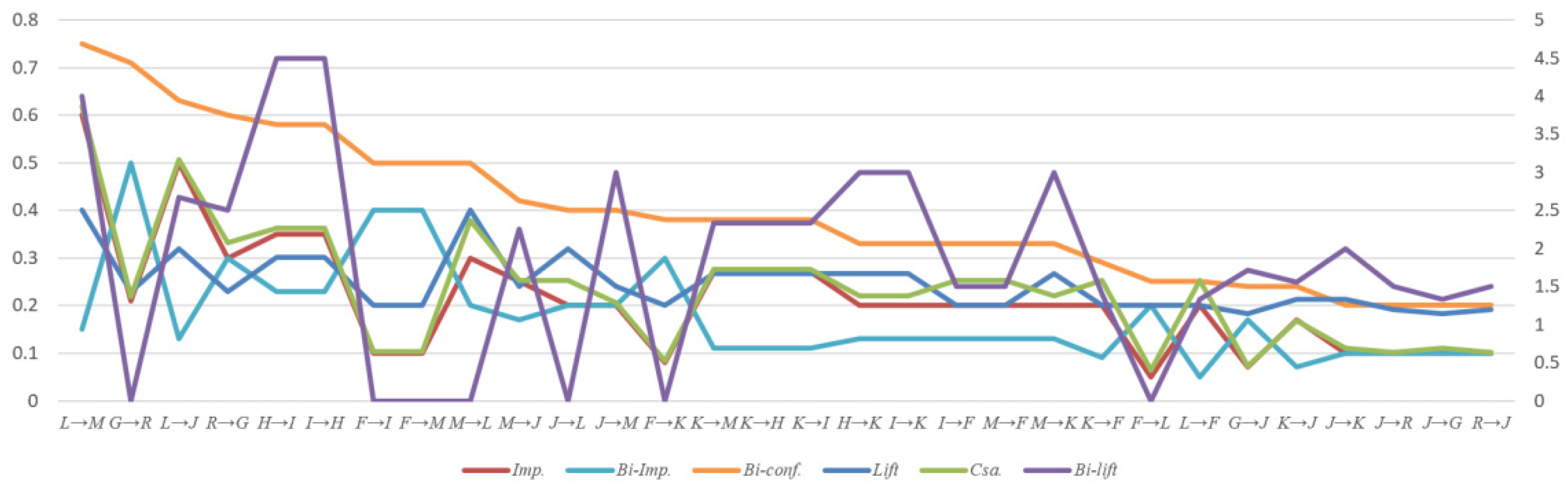
- The evaluation results of the author’s “Bi-confidence”, which is adjusted by the nonoccurrence probability of the antecedent, will increase the differentiation and accuracy. The novel Bi-support and Bi-confidence framework is more efficient than the traditional Support-confidence framework. The comparative results of the two different frameworks are shown in Table 7. There are nine rules that are useless (five rules have a negative correlation, and four rules have no correlation) in the Support-confidence framework. The new framework retains 12 high-value association rules of the old framework and reduces 32 non-value association rules. The high-value association rules are shown in Table 8 and Table 9. Evaluation results and comparisons of Improvement (Imp.), Bi-improvement (Bi-Imp.), Bi-confidence (Bi-conf.), Lift, Chi-square analysis (Csa.), and Bi-lift are shown in Figure 1.
According to the evaluation results and the performance analysis for the measurement method, the Validity (Val.) is not effective, and it can even lead to some essential mistakes under some circumstances. For instance, sometimes, when the evaluation shows negative, but the actual result shows to be positive.
Though essential mistakes would not occur in the Improvement (Imp.) and Chi-square analysis (Csa.), the stability of their evaluation still needs further improvement since they are likely to produce errors in calculation. Bi-lift has a small problem, as its premise is , and A and B are not certain events or impossible events. The evaluation results of the “Bi-confidence” could help improve the differentiation and accuracy, and the results show its high stability of evaluations. In conclusion, we can leave out indicators, such as Validity (Val.), Improvement (Imp.), Chi-square analysis (Csa.), Lift, and Bi-lift while we try to build up a reasonable measurement framework based on the indicators of Support, Confidence, and Bi-confidence. Procedures are as follows: firstly, use the Support threshold and Confidence threshold to filter out the frequent set, Supp() min supp, Supp() min supp, and conf () min conf; secondly, calculate the Bi-confidence value, and select rules by Bi-conf () min Bi-conf.
To sum up, in this paper, we propose an improved evaluation methodology for mining association rules. However, given that only a small number of data are used in verification, the new method and the new framework need to be further tested through the analysis of practical cases in the following studies.
5.2. Verification Analysis of Public Data Sets
In order to test the rationality and stability of the Bi-directional measure framework of association rules, this paper uses the public built-in data set of IBM SPSS Modeler for verification. The data set consists of more than 1000 shopping records with 11 items, including fruits, fresh meat, dairy products, and so on. Each shopping record contains 1 to 11 items. This paper uses traditional methods and Bi-support and Bi-confidence framework to generate association rules and verifies the stability of the Bi-support and Bi-confidence framework in removing low-value and valueless association rules. When the amount of data becomes larger, it is necessary to reduce the Confidence threshold or Support threshold to generate sufficient association rules, or the valuable association rules will be lost. If the Support threshold is maintained at 0.2, as mentioned above, less than 10 association rules are mined, failing to validate the ability of the Bi-support and Bi-confidence framework to remove low-value and valueless association rules. Therefore, this paper adjusts the Support threshold to 0.05, generating 72 association rules.
The comparative results of two different frameworks are shown in Table 10. Of the 72 association rules mined in the Support-Confidence framework, only 10 are of high value, but 48 are invalid. In the Bi-support and Bi-confidence framework, 48 invalid association rules are successfully filtered out, and 10 high-value association rules are retained. High-value association rules are shown in Table 11.
The bi-directional measure framework of association rules can stably remove low-value association rules and retain high-value rules in the verification of a small volume of data (11 instances, 10 pieces of data) and medium volume of data (11 instances, 1000 pieces of data). In order to test whether the bi-directional measure framework of association rules can perform well in the case of a large number of data, we use a groceries data set (https://github.com/stedy/Machine-Learning-with-R-datasets/blob/master/groceries.csv accessed in February 2021), which is a real transaction record of a grocery store for one month, with a total of 9835 consumption records and 169 items. The comparative results of the two different frameworks are shown in Table 12. There are 55 association rules with no value or low value among the 114 association rules mined in the Support-Confidence framework, while in the Bi-support and Bi-confidence framework, there are only 7 association rules with no value or low value, and 50 high-value association rules are retained.
6. Conclusions
This paper presents several key indicators for analyzing and comparing the various measures developed in the statistics and data mining literature. Given differences in some of their indicators, a significant number of these measures may provide conflicting information about the interestingness of rules. Therefore, how to estimate the reliability of the obtained association rules has become a research hotspot. We demonstrate the benefits of using Support in eliminating irrelevant and poorly correlated patterns. Studying the traditional association rules mining relies on the Support-confidence framework, and only rules that meet both the Support-Confidence threshold can be called strong association rules. However, sometimes strong association rules are of no interest to users, and even worse, these association rules can be misleading to some extent. Thus, in order to find the most valuable association rules, it is necessary to further analyze and evaluate the mined rules. Finally, we build up a reasonable measure framework (Bi-support and Bi-confidence framework) for mining appropriate association rules.
After mining association rules, how to judge the value of the mined rules is another hot topic. Generally, since most rules with high Support are either obvious or known to users, rules with low Support, bringing users something new, may outperform the former in terms of novelty. However, a relatively low Support threshold can also give rise to the combination explosion. Thus, the best way to resolve this dilemma is to set a low Support threshold first or use the dynamic Support threshold to complete a series of mining and then employ the new association rules measure framework to screen the mining results and extract the most valuable and interesting association rules at the same time. The new association rule measurement framework has high accuracy and stability for the screening and selecting of association rules. Moreover, it can be widely used for mixed or combined recommendations in commercial areas.
Although our proposed method improves the accuracy of the traditional interestingness measure methods and framework, it suffers from two limitations. The first limitation is that the experiment did not test for massive data. The second limitation is that the limited experimental results in various related fields. In the future, we will design parallel methods to deal with massive data and apply our findings to various related fields to observe their robustness [34,35,36,37,38,39,40,41].
Author Contributions
F.B. and C.X. (Chonghuan Xu). designed the study and conceived the manuscript. L.M. carried out the simulation experiments. F.B. and L.M. drafted the manuscript. F.B., C.X. (Chonghuan Xu), Y.Z. and C.X. (Cancan Xiao) were involved in revising the manuscript. All authors have read and agreed to the published version of the manuscript.
Funding
This research was supported by the Natural Science Foundation of Zhejiang Province (No. LQ20G010002), the National Natural Science Foundation of China (No. 71571162), the project of China (Hangzhou) cross-border electricity business school (No. 2021KXYJ06), and the Contemporary Business and Trade Research Center of Zhejiang Gongshang University (No. 2021SM05YB).
Institutional Review Board Statement
Not applicable.
Informed Consent Statement
Not applicable.
Data Availability Statement
The data used to support the findings of this study are available from the corresponding author upon request.
Conflicts of Interest
The authors declare that there is no conflict of interest.
References
- Herawan, T.; Dens, M. A Soft Set Approach for Association Rules Mining. Knowl.-Based Syst. 2011, 24, 186–195. [Google Scholar] [CrossRef]
- Kaushik, M.; Sharma, R.; Peious, S.; Shahin, M.; Yahia, S.; Draheim, D. A Systematic Assessment of Numerical Association Rule Mining Methods. SN Comput. Sci. 2021, 2, 348. [Google Scholar] [CrossRef]
- Zhao, Z.; Jian, Z.; Gaba, G.; Alroobaea, R.; Masud, M.; Rubaiee, S. An improved association rule mining algorithm for large data. J. Intell. Syst. 2021, 30, 750–762. [Google Scholar] [CrossRef]
- Wang, H.; Gao, Y. Research on parallelization of Apriori algorithm in association rule mining. Procedia Comput. Sci. 2021, 183, 641–647. [Google Scholar] [CrossRef]
- Telikani, A.; Gandomi, A.; Shahbahrami, A. A survey of evolutionary computation for association rule mining. Inf. Sci. 2020, 524, 318–352. [Google Scholar] [CrossRef]
- Fowler, J.H.; Laver, M. A Tournament of Party Decision Rules. J. Confl. Resolut. 1998, 52, 68–92. [Google Scholar] [CrossRef]
- Varija, B.; Hegde, N.P. An Association Mining Rules Implemented in Data Mining. Smart Innov. Syst. Technol. 2021, 225, 297–303. [Google Scholar]
- Srikand, B.R. Mining generalized association rules. Future Gener. Comput. Syst. 1997, 13, 161–180. [Google Scholar] [CrossRef]
- Arour, K.; Belkahla, A. Frequent Pattern-growth Algorithm on Multi-core CPU and GPU Processors. J. Comput. Inf. Technol. 2014, 22, 159–169. [Google Scholar] [CrossRef] [Green Version]
- Tseng, M.C.; Lin, W.Y.; Jeng, R. Incremental Maintenance of Generalized Association Rules under Taxonomy Evolution. J. Inf. Sci. 2008, 34, 174–195. [Google Scholar] [CrossRef]
- Marijana, Z.S.; Adela, H. Data Mining as Support to Knowledge Management in Marketing. Bus. Syst. Res. 2015, 6, 18–30. [Google Scholar]
- Chen, M.C. Ranking Discovered Rules from Data Mining with Multiple Criteria by Data Envelopment Analysis. Expert Syst. Appl. 2007, 33, 1100–1106. [Google Scholar] [CrossRef]
- Toloo, M.; Sohrabi, B.; Nalchigar, S. A New Method for Ranking Discovered Rules from Data Mining by DEA. Expert Syst. Appl. 2009, 36, 8503–8508. [Google Scholar] [CrossRef]
- Geng, L.; Hamilton, H.J. Interestingness Measures for Data Ming: A Survey. ACM Comput. Surv. 2006, 38, 9–es. [Google Scholar] [CrossRef]
- Hoque, N.; Nath, B.; Bhattacharyya, D.K. A New Approach on Rare Association Rule Mining. Int. J. Comput. Appl. 2012, 53, 297–303. [Google Scholar] [CrossRef] [Green Version]
- Zhang, J.; Wang, Y.; Feng, J. Attribute Index and Uniform Design Based Multiobjective Association Rule Mining with Evolutionary Algorithm. Sci. World J. 2013, 1, 1–16. [Google Scholar] [CrossRef]
- Pal, A.; Kumar, M. Distributed synthesized association mining for big transactional data. Sadhana 2020, 45, 169. [Google Scholar] [CrossRef]
- Huo, W.; Fang, X.; Zhang, Z. An Efficient Approach for Incremental Mining Fuzzy Frequent Itemsets with FP-Tree. Int. J. Uncertain. Fuzziness Knowl.-Based Syst. 2016, 24, 367–386. [Google Scholar] [CrossRef]
- Liu, L.; Wen, J.; Zheng, Z.; Su, H. An improved approach for mining association rules in parallel using Spark Streaming. Int. J. Circuit Theory Appl. 2021, 49, 1028–1039. [Google Scholar] [CrossRef]
- Islam, M.R.; Liu, S.; Biddle, R.; Razzak, I.; Wang, X.; Tilocca, P.; Xu, G. Discovering dynamic adverse behavior of policyholders in the life insurance industry. Technol. Forecast. Soc. Change 2021, 163, 120486. [Google Scholar] [CrossRef]
- Yang, D.; Nie, Z.T.; Yang, F. Time-Aware CF and Temporal Association Rule-Based Personalized Hybrid Recommender System. J. Organ. End User Comput. 2021, 33, 19–36. [Google Scholar] [CrossRef]
- Sanmiquel, L.; Bascompta, M.; Rossell, J.M.; Anticoi, H.F.; Guash, E. Analysis of Occupational Accidents in Underground and Surface Mining in Spain Using Data-Mining Techniques. Int. J. Environ. Res. Public Health 2018, 15, 462. [Google Scholar] [CrossRef] [Green Version]
- Zhang, Y.; Yu, W.; Ma, X.; Ogura, H.; Ye, D. Multi-Objective Optimization for High-Dimensional Maximal Frequent Itemset Mining. Appl. Sci. 2021, 11, 8971. [Google Scholar] [CrossRef]
- Song, K.; Lee, K. Predictability-based collective class association rule mining. Expert Syst. Appl. 2017, 79, 1–7. [Google Scholar] [CrossRef]
- Heechang, P. A Proposal of Symmetrically Balanced Cross Entropy for Association Rule Evaluation. J. Korean Data Anal. Soc. 2018, 20, 681–691. [Google Scholar]
- Shaharanee, I.; Hadzic, F. Evaluation and optimization of frequent, closed and maximal association rule based classification. Stat. Comput. 2014, 24, 821–843. [Google Scholar] [CrossRef]
- Silverstein, C.; Brin, S.; Motwani, R. Beyond Market Baskets: Generalizing Association Rules to Dependence Rules. Data Min. Knowl. Discov. 1998, 2, 39–68. [Google Scholar] [CrossRef]
- Ma, L.; Jie, W. Research on Judgment Criterion of Association Rules. Control. Decis. 2003, 18, 277–280. [Google Scholar]
- Brin, S.; Motwani, R.; Ullman, J.D.; Tsur, S. Dynamic Itemset Counting and Implication Rules for Market Basket Data. In Proceedings of the 1997 ACM SIGMOD International Conference on Management of Data, Tucson, AZ, USA, 11–15 May 1997; pp. 255–264. [Google Scholar]
- Li, Y.; Wu, C.; Wang, K. A New Interestingness Measures for Ming Association Rules. J. China Soc. Sci. Tech. Inf. 2011, 30, 503–507. [Google Scholar]
- Bao, F.; Wu, Y.; Li, Z.; Li, Y.; Liu, L.; Chen, G. Effect Improved for High-Dimensional and Unbalanced Data Anomaly Detection Model Based on KNN-SMOTE-LSTM. Complexity 2020. [Google Scholar] [CrossRef]
- Lenca, P.; Meyer, P.; Vaillant, B. On Selecting Interestingness Measures for Association Rules: User Oriented Description and Multiple Criteria Decision Aid. Eur. J. Oper. Res. 2008, 184, 610–626. [Google Scholar] [CrossRef] [Green Version]
- Ju, C.; Bao, F.; Xu, C.; Fu, X. A Novel Method of Interestingness Measures for Association Rules Mining Based on Profit. Discret. Dyn. Nat. Soc. 2015, 1, 1–10. [Google Scholar] [CrossRef] [Green Version]
- Adomavicius, G.; Tuzhilin, A. Toward the next generation of recommender systems: A survey of the state-of-the-art and possible extensions. IEEE Trans. Knowl. Data Eng. 2005, 17, 734–749. [Google Scholar] [CrossRef]
- Xiang, K.; Xu, C.; Wang, J. Understanding the Relationship Between Tourists’ Consumption Behavior and Their Consumption Substitution Willingness Under Unusual Environment. Psychol. Res. Behav. Manag. 2021, 14, 483–500. [Google Scholar] [CrossRef]
- Wang, J.; Xu, C.; Liu, W. Understanding the adoption of mobile social payment? From the cognitive behavioral perspective. Int. J. Mob. Commun. 2022; in press. [Google Scholar] [CrossRef]
- Xu, C.; Ding, A.S.; Zhao, K. A novel POI recommendation method based on trust relationship and spatial-temporal factors. Electron. Commer. Res. Appl. 2021, 48, 101060. [Google Scholar] [CrossRef]
- Xu, C.; Liu, D.; Mei, X. Exploring an Efficient POI Recommendation Model Based on User Characteristics and Spatial-Temporal Factors. Mathematics 2021, 9, 2673. [Google Scholar] [CrossRef]
- Tang, Z.; Hu, H.; Xu, C. A federated learning method for network intrusion detection. Concurr. Comput. Pract. Exp. 2022, e6812. [Google Scholar] [CrossRef]
- Xu, C.; Ding, A.S.; Liao, S.S. A privacy-preserving recommendation method based on multi-objective optimisation for mobile users. Int. J. Bio-Inspired Comput. 2020, 16, 23–32. [Google Scholar] [CrossRef]
- Chen, Y.; Thaipisutikul, T.; Shih, T.K. A Learning-Based POI Recommendation with Spatiotemporal Context Awareness. IEEE Trans. Cybern 2020, 99, 1–14. [Google Scholar] [CrossRef] [PubMed]
Figure 1.
Evaluation results and comparisons of Improvement (Imp.), Bi-improvement (Bi-Imp.), Bi-confidence (Bi-conf.), Lift, Chi-square analysis (Csa.), and Bi-lift.
Figure 1.
Evaluation results and comparisons of Improvement (Imp.), Bi-improvement (Bi-Imp.), Bi-confidence (Bi-conf.), Lift, Chi-square analysis (Csa.), and Bi-lift.


Table 1.
A data set of transaction.
| Tid | E | F | G | H | I | J | K | L | M | N | R | Total |
|---|---|---|---|---|---|---|---|---|---|---|---|---|
| 1 | 1 | 1 | 1 | 1 | 1 | 1 | 1 | 0 | 1 | 0 | 0 | 8 |
| 2 | 1 | 1 | 0 | 1 | 1 | 1 | 1 | 1 | 1 | 0 | 0 | 8 |
| 3 | 1 | 1 | 0 | 1 | 1 | 0 | 0 | 0 | 0 | 1 | 0 | 5 |
| 4 | 1 | 1 | 1 | 0 | 0 | 1 | 0 | 1 | 1 | 1 | 1 | 8 |
| 5 | 1 | 1 | 1 | 0 | 0 | 1 | 0 | 0 | 0 | 1 | 1 | 6 |
| 6 | 1 | 1 | 1 | 0 | 0 | 0 | 0 | 0 | 1 | 1 | 1 | 6 |
| 7 | 1 | 1 | 0 | 0 | 0 | 0 | 1 | 0 | 0 | 1 | 0 | 4 |
| 8 | 1 | 1 | 1 | 0 | 1 | 0 | 0 | 0 | 0 | 0 | 1 | 5 |
| 9 | 1 | 0 | 1 | 1 | 0 | 0 | 0 | 0 | 0 | 1 | 0 | 4 |
| 10 | 1 | 0 | 1 | 0 | 0 | 1 | 0 | 0 | 0 | 0 | 1 | 4 |
| Total | 10 | 8 | 7 | 4 | 4 | 5 | 3 | 2 | 4 | 6 | 5 | 58 |
Table 2.
The occurrence of “A” and “B”.
| Occur | Not Occur | Total | |
|---|---|---|---|
| occur | 50 | 30 | 80 |
| not occur | 20 | 0 | 20 |
| Total | 70 | 30 | 100 |
Table 3.
The occurrence of “A” and “B”.
| Total | |||
|---|---|---|---|
| occur | 825 | 75 | 900 |
| not occur | 50 | 50 | 100 |
| Total | 875 | 125 | 1000 |
Table 4.
The occurrence of “C” and “D”.
| D Occur | D Not Occur | Total | |
|---|---|---|---|
| C occur | 345 | 55 | 400 |
| C not occur | 385 | 215 | 600 |
| Total | 730 | 270 | 1000 |
Table 5.
Rules list with the Support-confidence framework (min supp. = 0.2, min conf. = 0.5).
| Rules | Supp. | Conf. | Lift | Val. | Conv. | Imp. | Csa. | Bi-lift | Bi-imp. | Bi-conf. |
|---|---|---|---|---|---|---|---|---|---|---|
| M→J | 0.3 | 0.75 | 1.5 | 0.1 | 2 | 0.25 | 1.58 | 2.25 | 0.16 | 0.42 |
| M→G | 0.3 | 0.75 | 1.08 | 0.1 | 1.2 | 0.05 | 0.35 | 1.13 | 0.03 | 0.08 |
| J→G | 0.4 | 0.8 | 1.14 | 0.1 | 0.75 | 0.1 | 0.69 | 1.33 | 0.1 | 0.2 |
| I→H | 0.3 | 0.75 | 1.88 | 0.2 | 2.4 | 0.35 | 2.26 | 4.5 | 0.23 | 0.58 |
| I→F | 0.4 | 1 | 1.25 | 0 | / | 0.2 | 1.58 | 1.5 | 0.13 | 0.33 |
| H→F | 0.3 | 0.75 | 0.95 | −0.2 | 0.8 | −0.05 | −0.4 | 0.9 | −0.03 | −0.08 |
| R→G | 0.5 | 1 | 1.42 | 0.3 | / | 0.3 | 2.1 | 2.5 | 0.3 | 0.6 |
| N→G | 0.4 | 0.67 | 0.95 | 0.1 | 0.9 | −0.03 | −0.21 | 0.89 | −0.05 | −0.08 |
| R→F | 0.4 | 0.8 | 1 | 0 | 1 | 0 | 0 | 1 | 0 | 0 |
| N→F | 0.5 | 0.83 | 1.04 | 0.2 | 1.2 | 0.03 | 0.24 | 1.11 | 0.05 | 0.08 |
| M→F | 0.4 | 1 | 1.25 | 0 | / | 0.2 | 1.58 | 1.5 | 0.13 | 0.33 |
| J→F | 0.4 | 0.8 | 1 | 0 | 1 | 0 | 0 | 1 | 0 | 0 |
| G→F | 0.5 | 0.71 | 0.89 | 0.2 | 0.7 | −0.09 | −0.71 | 0.71 | −0.21 | −0.28 |
| J→M | 0.3 | 0.6 | 1.5 | 0.2 | 1.5 | 0.2 | 1.29 | 3 | 0.2 | 0.4 |
| G→J | 0.4 | 0.57 | 1.14 | 0.3 | 1.17 | 0.07 | 0.44 | 1.71 | 0.18 | 0.24 |
| H→I | 0.3 | 0.75 | 1.88 | 0.2 | 2.4 | 0.35 | 2.26 | 4.5 | 0.23 | 0.58 |
| F→I | 0.4 | 0.5 | 1.25 | 0.4 | 1.2 | 0.1 | 0.65 | / | 0.4 | 0.5 |
| G→R | 0.5 | 0.71 | 1.42 | 0.5 | 1.75 | 0.21 | 1.33 | / | 0.49 | 0.71 |
| G→N | 0.4 | 0.57 | 0.95 | 0.2 | 0.93 | −0.03 | −0.19 | 0.86 | −0.07 | −0.1 |
| F→R | 0.4 | 0.5 | 1 | 0.3 | 1 | 0 | 0 | 1 | 0 | 0 |
| F→N | 0.5 | 0.63 | 1.04 | 0.4 | 1.07 | 0.03 | 0.19 | 1.25 | 0.12 | 0.13 |
| F→M | 0.4 | 0.5 | 1.25 | 0.4 | 1.2 | 0.1 | 0.65 | / | 0.4 | 0.5 |
| F→J | 0.4 | 0.5 | 1 | 0.3 | 1 | 0 | 0 | 1 | 0 | 0 |
| F→G | 0.5 | 0.63 | 0.89 | 0.3 | 0.8 | −0.07 | −0.48 | 0.63 | −0.28 | −0.38 |
| M→L | 0.2 | 0.5 | 2.5 | 0.2 | 0.64 | 0.3 | 2.37 | / | 0.2 | 0.5 |
Table 6.
Rules list with the new framework (min supp.(AB) = 0.2, min supp.() = 0.2, min conf. = 0.2, and Bi-conf. = 0.2).
Table 6.
Rules list with the new framework (min supp.(AB) = 0.2, min supp.() = 0.2, min conf. = 0.2, and Bi-conf. = 0.2).
| Rules | Supp. AB | Supp. | Conf. | Lift | Imp. | Csa. | Bi-lift | Bi-Imp. | Bi-conf. |
|---|---|---|---|---|---|---|---|---|---|
| F→I | 0.4 | 0.2 | 0.50 | 1.25 | 0.10 | 0.65 | / | 0.40 | 0.50 |
| F→K | 0.3 | 0.2 | 0.38 | 1.25 | 0.08 | 0.52 | / | 0.30 | 0.38 |
| F→L | 0.2 | 0.2 | 0.25 | 1.25 | 0.05 | 0.40 | / | 0.20 | 0.25 |
| F→M | 0.4 | 0.2 | 0.50 | 1.25 | 0.10 | 0.65 | / | 0.40 | 0.50 |
| G→J | 0.4 | 0.2 | 0.57 | 1.14 | 0.07 | 0.45 | 1.71 | 0.17 | 0.24 |
| G→R | 0.5 | 0.3 | 0.71 | 1.43 | 0.21 | 1.36 | / | 0.50 | 0.71 |
| H→I | 0.3 | 0.5 | 0.75 | 1.88 | 0.35 | 2.26 | 4.50 | 0.23 | 0.58 |
| H→K | 0.2 | 0.5 | 0.50 | 1.67 | 0.20 | 1.38 | 3.00 | 0.13 | 0.33 |
| I→K | 0.2 | 0.5 | 0.50 | 1.67 | 0.20 | 1.38 | 3.00 | 0.13 | 0.33 |
| J→K | 0.2 | 0.4 | 0.40 | 1.33 | 0.10 | 0.69 | 2.00 | 0.10 | 0.20 |
| J→L | 0.2 | 0.5 | 0.40 | 2.00 | 0.20 | 1.58 | / | 0.20 | 0.40 |
| J→M | 0.3 | 0.4 | 0.60 | 1.50 | 0.20 | 1.29 | 3.00 | 0.20 | 0.40 |
| J→R | 0.3 | 0.3 | 0.60 | 1.20 | 0.10 | 0.63 | 1.50 | 0.10 | 0.20 |
| K→M | 0.2 | 0.5 | 0.67 | 1.67 | 0.27 | 1.72 | 2.33 | 0.11 | 0.38 |
| L→M | 0.2 | 0.6 | 1.00 | 2.50 | 0.60 | 3.87 | 4.00 | 0.15 | 0.75 |
| I→F | 0.4 | 0.2 | 1.00 | 1.25 | 0.20 | 1.58 | 1.50 | 0.13 | 0.33 |
| K→F | 0.3 | 0.2 | 1.00 | 1.25 | 0.20 | 1.58 | 1.40 | 0.09 | 0.29 |
| L→F | 0.2 | 0.2 | 1.00 | 1.25 | 0.20 | 1.58 | 1.33 | 0.05 | 0.25 |
| M→F | 0.4 | 0.2 | 1.00 | 1.25 | 0.20 | 1.58 | 1.50 | 0.13 | 0.33 |
| J→G | 0.4 | 0.2 | 0.80 | 1.14 | 0.10 | 0.69 | 1.33 | 0.10 | 0.20 |
| R→G | 0.5 | 0.3 | 1.00 | 1.43 | 0.30 | 2.07 | 2.50 | 0.30 | 0.60 |
| I→H | 0.3 | 0.5 | 0.75 | 1.88 | 0.35 | 2.26 | 4.50 | 0.23 | 0.58 |
| K→H | 0.2 | 0.5 | 0.67 | 1.67 | 0.27 | 1.72 | 2.33 | 0.11 | 0.38 |
| K→I | 0.2 | 0.5 | 0.67 | 1.67 | 0.27 | 1.72 | 2.33 | 0.11 | 0.38 |
| K→J | 0.2 | 0.4 | 0.67 | 1.33 | 0.17 | 1.05 | 1.56 | 0.07 | 0.24 |
| L→J | 0.2 | 0.5 | 1.00 | 2.00 | 0.50 | 3.16 | 2.67 | 0.13 | 0.63 |
| M→J | 0.3 | 0.4 | 0.75 | 1.50 | 0.25 | 1.58 | 2.25 | 0.17 | 0.42 |
| R→J | 0.3 | 0.3 | 0.60 | 1.20 | 0.10 | 0.63 | 1.50 | 0.10 | 0.20 |
| M→K | 0.2 | 0.5 | 0.50 | 1.67 | 0.20 | 1.38 | 3.00 | 0.13 | 0.33 |
| M→L | 0.2 | 0.6 | 0.50 | 2.50 | 0.30 | 2.37 | / | 0.20 | 0.50 |
Table 7.
Comparisons of the different frameworks.
| Framework | Conditions | High Value | Low Value | No Value | Total |
|---|---|---|---|---|---|
| support-confidence | min supp. (AB) = 0.2, and min conf. (AB) = 0.5 | 9 | 7 | 9 | 25 |
| support-confidence | min supp. (AB) = 0.2, and min conf. (AB) = 0.2 | 12 | 22 | 32 | 66 |
| Bi-support and Bi-confidence | min supp. (AB) = 0.2, min supp. ) = 0.2, min conf. (AB) = 0.2, and Bi-conf. (AB) = 0.2 | 12 | 18 | 0 | 30 |
Table 8.
Top 12 rules with the new framework (min supp.(AB) = 0.2, min supp.( ) = 0.2, min conf. = 0.2, and Bi-conf. = 0.2).
Table 8.
Top 12 rules with the new framework (min supp.(AB) = 0.2, min supp.( ) = 0.2, min conf. = 0.2, and Bi-conf. = 0.2).
| Rules | Supp. AB | Supp. | Conf. | Lift | Imp. | Csa. | Bi-lift | Bi-Imp. | Bi-conf. |
|---|---|---|---|---|---|---|---|---|---|
| L→M | 0.2 | 0.6 | 1.00 | 2.50 | 0.60 | 3.87 | 4.00 | 0.15 | 0.75 |
| G→R | 0.5 | 0.3 | 0.71 | 1.43 | 0.21 | 1.36 | 0.50 | 0.71 | |
| L→J | 0.2 | 0.5 | 1.00 | 2.00 | 0.50 | 3.16 | 2.67 | 0.13 | 0.63 |
| R→G | 0.5 | 0.3 | 1.00 | 1.43 | 0.30 | 2.07 | 2.50 | 0.30 | 0.60 |
| H→I | 0.3 | 0.5 | 0.75 | 1.88 | 0.35 | 2.26 | 4.50 | 0.23 | 0.58 |
| I→H | 0.3 | 0.5 | 0.75 | 1.88 | 0.35 | 2.26 | 4.50 | 0.23 | 0.58 |
| M→L | 0.2 | 0.6 | 0.50 | 2.50 | 0.30 | 2.37 | 0.20 | 0.50 | |
| F→I | 0.4 | 0.2 | 0.50 | 1.25 | 0.10 | 0.65 | 0.40 | 0.50 | |
| F→M | 0.4 | 0.2 | 0.50 | 1.25 | 0.10 | 0.65 | 0.40 | 0.50 | |
| M→J | 0.3 | 0.4 | 0.75 | 1.50 | 0.25 | 1.58 | 2.25 | 0.17 | 0.42 |
| J→L | 0.2 | 0.5 | 0.40 | 2.00 | 0.20 | 1.58 | 0.20 | 0.40 | |
| J→M | 0.3 | 0.4 | 0.60 | 1.50 | 0.20 | 1.29 | 3.00 | 0.40 |
Table 9.
Top 9 Rules with the Support-Confidence framework (min supp. = 0.2, min conf. = 0.5).
| Rules | Supp. | Conf. | Lift | Imp. | Csa. | Bi-lift | Bi-imp. | Bi-conf. |
|---|---|---|---|---|---|---|---|---|
| G→R | 0.5 | 0.71 | 1.42 | 0.21 | 1.33 | / | 0.49 | 0.71 |
| R→G | 0.5 | 1 | 1.42 | 0.3 | 2.1 | 2.5 | 0.3 | 0.6 |
| I→H | 0.3 | 0.75 | 1.88 | 0.35 | 2.26 | 4.5 | 0.23 | 0.58 |
| H→I | 0.3 | 0.75 | 1.88 | 0.35 | 2.26 | 4.5 | 0.23 | 0.58 |
| F→I | 0.4 | 0.5 | 1.25 | 0.1 | 0.65 | / | 0.4 | 0.5 |
| F→M | 0.4 | 0.5 | 1.25 | 0.1 | 0.65 | / | 0.4 | 0.5 |
| M→L | 0.2 | 0.5 | 2.5 | 0.3 | 2.37 | / | 0.2 | 0.5 |
| M→J | 0.3 | 0.75 | 1.5 | 0.25 | 1.58 | 2.25 | 0.16 | 0.42 |
| J→M | 0.3 | 0.6 | 1.5 | 0.2 | 1.29 | 3 | 0.2 | 0.4 |
Table 10.
Comparisons of the different frameworks with data from the IBM SPSS Modeler.
| Framework | Conditions | High Value | Low Value | No Value | Total |
|---|---|---|---|---|---|
| support-confidence | min supp. (AB) = 0.05, and min conf. (AB) = 0.2 | 10 | 14 | 48 | 72 |
| Bi-support and Bi-confidence | 10 | 5 | 0 | 15 |
Table 11.
Top 10 rules with the new framework (min supp.(AB) = 0.05, min supp.( ) = 0.05, min conf. = 0.2, and Bi-conf. = 0.2).
Table 11.
Top 10 rules with the new framework (min supp.(AB) = 0.05, min supp.( ) = 0.05, min conf. = 0.2, and Bi-conf. = 0.2).
| Rules | Supp. AB | Conf. | Bi-conf. | |
|---|---|---|---|---|
| Beer→Frozen meat | 0.29 | 0.57 | 0.58 | 0.39 |
| Frozen meat→beer | 0.30 | 0.57 | 0.56 | 0.39 |
| Frozen meat→Canned vegetables | 0.30 | 0.56 | 0.57 | 0.39 |
| Canned vegetables→Frozen meat | 0.30 | 0.56 | 0.57 | 0.39 |
| Beer→Canned vegetables | 0.29 | 0.57 | 0.57 | 0.38 |
| Canned vegetables→beer | 0.30 | 0.57 | 0.55 | 0.37 |
| Candy→wine | 0.27 | 0.58 | 0.52 | 0.32 |
| Wine→candy | 0.28 | 0.58 | 0.50 | 0.32 |
| Fish→Fruits and vegetables | 0.29 | 0.55 | 0.50 | 0.28 |
| Fruits and vegetables→fish | 0.29 | 0.55 | 0.48 | 0.28 |
| Beer→Frozen meat | 0.29 | 0.57 | 0.58 | 0.39 |
| Frozen meat→beer | 0.30 | 0.57 | 0.56 | 0.39 |
Table 12.
Comparisons of different Framework with Groceries data set.
| Framework | Conditions | High Value | Low Value | No Value | Total |
|---|---|---|---|---|---|
| support-confidence | min supp. (AB) = 0.02, and min conf. (AB) = 0.1 | 59 | 37 | 18 | 114 |
| Bi-support and Bi-confidence | min supp. (AB) = 0.02 min supp. ) = 0.02, min conf. (AB) = 0.1 and Bi-conf. (AB) = 0.1 | 50 | 7 | 0 | 57 |
Publisher’s Note: MDPI stays neutral with regard to jurisdictional claims in published maps and institutional affiliations. |
© 2021 by the authors. Licensee MDPI, Basel, Switzerland. This article is an open access article distributed under the terms and conditions of the Creative Commons Attribution (CC BY) license (https://creativecommons.org/licenses/by/4.0/).
Share and Cite
MDPI and ACS Style
Bao, F.; Mao, L.; Zhu, Y.; Xiao, C.; Xu, C. An Improved Evaluation Methodology for Mining Association Rules. Axioms 2022, 11, 17. https://doi.org/10.3390/axioms11010017
AMA Style
Bao F, Mao L, Zhu Y, Xiao C, Xu C. An Improved Evaluation Methodology for Mining Association Rules. Axioms. 2022; 11(1):17. https://doi.org/10.3390/axioms11010017
Chicago/Turabian StyleBao, Fuguang, Linghao Mao, Yiling Zhu, Cancan Xiao, and Chonghuan Xu. 2022. "An Improved Evaluation Methodology for Mining Association Rules" Axioms 11, no. 1: 17. https://doi.org/10.3390/axioms11010017
Note that from the first issue of 2016, this journal uses article numbers instead of page numbers. See further details here.