Theory of the Anomalous Magnetic Moment of the Electron

Abstract

The anomalous magnetic moment of the electron $a_e$ measured in a Penning trap occupies a unique position among high precision measurements of physical constants in the sense that it can be compared directly with the theoretical calculation based on the renormalized quantum electrodynamics (QED) to high orders of perturbation expansion in the fine structure constant $\alpha$, with an effective parameter $\alpha /\pi$. Both numerical and analytic evaluations of $a_e$ up to ${(\alpha /\pi )}^4$ are firmly established. The coefficient of ${(\alpha /\pi )}^5$ has been obtained recently by an extensive numerical integration. The contributions of hadronic and weak interactions have also been estimated. The sum of all these terms leads to $a_e\left(\mathrm{theory}\right)$ = $1159652181.606\left(11\right)\left(12\right)\left(229\right)\times {10}^{-12}$, where the first two uncertainties are from the tenth-order QED term and the hadronic term, respectively. The third and largest uncertainty comes from the current best value of the fine-structure constant derived from the cesium recoil measurement: ${\alpha }^{-1}\left(\mathrm{Cs}\right)=137.035999046\left(27\right)$. The discrepancy between $a_e\left(\mathrm{theory}\right)$ and $a_e\left(\left(\mathrm{experiment}\right)\right)$ is 2.4$\sigma$. Assuming that the standard model is valid so that $a_e$(theory) = $a_e$(experiment) holds, we obtain ${\alpha }^{-1}\left(a_e\right)=137.0359991496\left(13\right)\left(14\right)\left(330\right)$, which is nearly as accurate as ${\alpha }^{-1}\left(\mathrm{Cs}\right)$. The uncertainties are from the tenth-order QED term, hadronic term, and the best measurement of $a_e$, in this order.

1. Introduction

The anomalous magnetic moment of the electron was discovered in 1947 by P. Kusch and H. M. Foley [1]. The Zeeman spectra of the gallium atom in a constant magnetic field were measured, and the gyromagnetic ratio (g value) of the electron was determined. If the orbital g value is assumed to be one as Dirac theory predicts, the spin g value of the electron is determined to be

$$g=2\times (1.00119\pm 0.00005).$$

(1)

The g value of the electron derived from the Dirac theory is exactly an integer two, and the difference between the measured g value and Dirac’s two is called the anomalous magnetic moment of the electron:

$$a_e\equiv (g-2)/2=0.00119\left(5\right).$$

(2)

This tiny 0.1% deviation of the electron g, as well as the Lamb shift of the hydrogen atom discovered one year earlier [2] were the achievements of the state-of-the-art improvements in the frequency measurements at that time.

Theory of charged particles and photons, named as quantum electrodynamics (QED), was also developed in the same era. It must be distinguished from its old version from the 1920s, which suffered from the divergence problem associated with perturbative calculation [3,4]. The new idea, renormalization, enables us to compute finite physical quantities from the perturbation theory of QED with high precision. J. Schwinger showed that the value of the anomalous magnetic moment of the electron $a_e$ can be attributed to the one-loop effect of QED [5]. Precision comparison between measurement and theory in 1947–1948 was the starting point of stringent tests of QED and the standard model of elementary particles. The very high precision achieved in testing $a_e$ is a consequence of small values of the fine structure constant $\alpha$ and the small electron mass. The Lamb shift could not serve as the high precision test of QED since it depends on other quantities such as hadronic interactions and hadronic masses.

In this article, we review the current status of the theory of the electron anomalous magnetic moment, including the contribution of Feynman diagrams of QED up to the tenth-order perturbation theory. Of course, our starting points are Feynman diagrams and corresponding integrals. However, these integrals, usually defined in the momentum space, are not convenient for numerical integration. Thus, we transform them to forms accessible to numerical integration. Currently, the numerical integration method is the only way to approach the tenth-order QED Feynman diagrams. The numerical computation methods of QED have been given in several references: our approach is given in [6,7,8,9,10,11,12], and alternatives are found in [13,14,15]. In Section 2, the contributions to $a_e$ from all known sources are listed. In the subsequent sections, step-by-step instructions are given for the conversion of Feynman integrals to one accessible to numerical integration, working on the fourth-order diagrams as an example.

2. Summary of Contributions to ${\mathit{a}}_{\mathit{e}}$

Before digging into the calculation method of a Feynman diagram, let us summarize the theoretical value of the electron anomalous magnetic moment $a_e$. The standard model contribution to $a_e$ can be divided into three terms:

$$a_e=a_e\left(\mathrm{QED}\right)+a_e\left(\mathrm{weak}\right)+a_e\left(\mathrm{hadron}\right).$$

(3)

The QED contribution $a_e\left(\mathrm{QED}\right)$ involves the leptons, which are electron (e), muon ($\mu$), and tau ($\tau$), and photons. The contribution involving the weak bosons ($W^{\pm },Z^0$) is categorized into $a_e\left(\mathrm{weak}\right)$. The contribution from quarks or hadrons without a weak boson is denoted by $a_e\left(\mathrm{hadron}\right)$. Since the electron is much lighter than the weak bosons and hadrons, the QED contribution dominates over others: $a_e\left(\mathrm{weak}\right)$ and $a_e\left(\mathrm{hadron}\right)$ amount to only 0.026 ppb [16,17,18,19] and 1.47 ppb [20,21,22], respectively, of the whole contribution.

The QED contribution is further divided according to its lepton-mass dependence. Since the anomaly $a_e$ is dimensionless, lepton-mass dependence appears in the form of the ratio between lepton masses. Thus, we may rewrite

$$a_e\left(\mathrm{QED}\right)=A_1+A_2(m_e/m_{\mu })+A_2(m_e/m_{\tau })+A_3(m_e/m_{\mu },m_e/m_{\tau }),$$

(4)

where $m_e$, $m_{\mu }$, and $m_{\tau }$ are masses of the electron, muon, and tau-lepton, respectively. The term $A_1$ is independent of the lepton-mass ratios and universal for all lepton species.

Both mass-independent and mass-dependent terms can be calculated in a framework of the perturbation series expressed by Feynman diagrams. The expansion parameter of the perturbation series is the coupling constant of QED, namely the elementary charge e of leptons. Since it involves only even powers of e, the perturbation expansion is expressed in terms of the fine-structure constant $\alpha$, which is proportional to $e^2$. Thus, a Feynman diagram with n-loops appears in the $2n\mathrm{th}$-order of the perturbation series of QED.

In SI units, the fine-structure constant $\alpha$ is defined as

$$\alpha =\frac{e^2}{4\pi {ϵ}_0\hslash c},$$

(5)

where ℏ is the Dirac constant, which is the Planck constant h divided by $2\pi$, c is the speed of light, and ${ϵ}_0$ is the electric constant. As is well known, in the current SI system, c and ${ϵ}_0$ are the defined constants. The new SI will be launched in May 2019, and the Planck constant h and the elementary charge e will become the defined constants, while the electric constant ${ϵ}_0$ will no longer be a defined constant.

In the natural units $c=\hslash ={ϵ}_0=1$, the fine-structure constant has a much simpler expression:

$$\alpha =\frac{e^2}{4\pi }.$$

(6)

Hereafter, we shall use the natural units. Since the fine-structure constant $\alpha$ is a dimensionless constant, it has the same value regardless of the chosen units.

Since measurements find that $\alpha =1/137.035\dots$, we are lucky enough to have an effective perturbation series for QED calculation:

$$A_i=\left(\frac{\alpha }{\pi }\right)A_i^{\left(2\right)}+{\left(\frac{\alpha }{\pi }\right)}^2{A}_i^{\left(4\right)}+{\left(\frac{\alpha }{\pi }\right)}^3{A}_i^{\left(6\right)}+\cdots ,\mathrm{for}i=1,2,3.$$

(7)

Because of the renormalizability of QED, every $A_i^{\left(2n\right)}$ is finite and calculable by using the Feynman-diagram techniques. The results of QED calculation are summarized in

Table 1. QED contributions to the electron anomalous magnetic moment $a_e$. The coefficients of ${(\alpha /\pi )}^n$, $A_i^{\left(2n\right)}$, where n denotes the $2n\mathrm{th}$-order of the perturbation theory of QED, are listed. No input parameter is used to compute $A_1^{\left(2n\right)}$, while the electron-to-muon mass ratio $m_e/m_{\mu }=$ 0.483 633 170 (11) $\times {10}^{-2}$ [41] and the electron-to-tau mass ratio $m_e/m_{\tau }=0.287585\left(19\right)\times {10}^{-3}$ [42] are used for $A_2^{\left(2n\right)}$ and $A_3^{\left(2n\right)}$. The assigned uncertainties for the fourth-, sixth-, and eighth-order mass-dependent terms come from the lepton-mass ratios. The uncertainties of the tenth-order terms are due to numerical integration. The tau-lepton contributions to the tenth-order term have not yet been calculated, but they are suppressed by the factor ${(m_{\mu }/m_{\tau })}^2$ compared with the muon contributions.

Coefficient ${\mathit{A}}_{\mathit{i}}^{\left(2\mathit{n}\right)}$	Value (Error)	References
$A_1^{\left(2\right)}$	0.5	[5]
$A_2^{\left(2\right)}(m_e/m_{\mu })$	0
$A_2^{\left(2\right)}(m_e/m_{\tau })$	0
$A_3^{\left(2\right)}(m_e/m_{\mu },m_e/m_{\tau })$	0
$A_1^{\left(4\right)}$	−0.328 478 965 579 193⋯	[23,24]
$A_2^{\left(4\right)}(m_e/m_{\mu })$	0.519 738 676 (24) × 10−6	[27]
$A_2^{\left(4\right)}(m_e/m_{\tau })$	0.183 790 (25) × 10−8	[27]
$A_3^{\left(4\right)}(m_e/m_{\mu },m_e/m_{\tau })$	0
$A_1^{\left(6\right)}$	1.181 241 456 587⋯	[25,33]
$A_2^{\left(6\right)}(m_e/m_{\mu })$	−0.737 394 164 (24) × 10−5	[28,29,30,31]
$A_2^{\left(6\right)}(m_e/m_{\tau })$	−0.658 273 (79) × 10−7	[28,29,30,31]
$A_3^{\left(6\right)}(m_e/m_{\mu },m_e/m_{\tau })$	0.1909 (1) × 10−12	[43]
$A_1^{\left(8\right)}$	−1.912 245 764⋯	[26,39]
$A_2^{\left(8\right)}(m_e/m_{\mu })$	0.916 197 070 (37) × 10−3	[32,35]
$A_2^{\left(8\right)}(m_e/m_{\tau })$	0.742 92 (12) × 10−5	[32,35]
$A_3^{\left(8\right)}(m_e/m_{\mu },m_e/m_{\tau })$	0.746 87 (28) × 10−6	[32,35]
$A_1^{\left(10\right)}$	6.737 (159)	new, [40]
$A_2^{\left(10\right)}(m_e/m_{\mu })$	−0.003 82 (39)	[35,39]
$A_2^{\left(10\right)}(m_e/m_{\tau })$	$\mathcal{O}\left({10}^{-5}\right)$
$A_3^{\left(10\right)}(m_e/m_{\mu },m_e/m_{\tau })$	$\mathcal{O}\left({10}^{-5}\right)$

. By now, all coefficients $A_i^{\left(2n\right)}$ up to the eighth-order have been found analytically [5,23,24,25,26,27,28,29,30,31,32]. They are consistent with numerical evaluations [33,34,35]. The references quoted here are responsible only for the final stages of the calculation of each term, which were built upon much effort of many scientists over seventy years. Note that the mass-dependent terms of the sixth- and eighth-order terms, $A_2^{\left(6\right)}$, $A_2^{\left(8\right)}$, are not given in the closed forms. However, sufficiently higher order terms of the series expansion in a mass ratio were analytically obtained [30,31,32]. Furthermore, the mass-independent eighth-order term $A_1^{\left(8\right)}$ in [26] is not fully analytic.

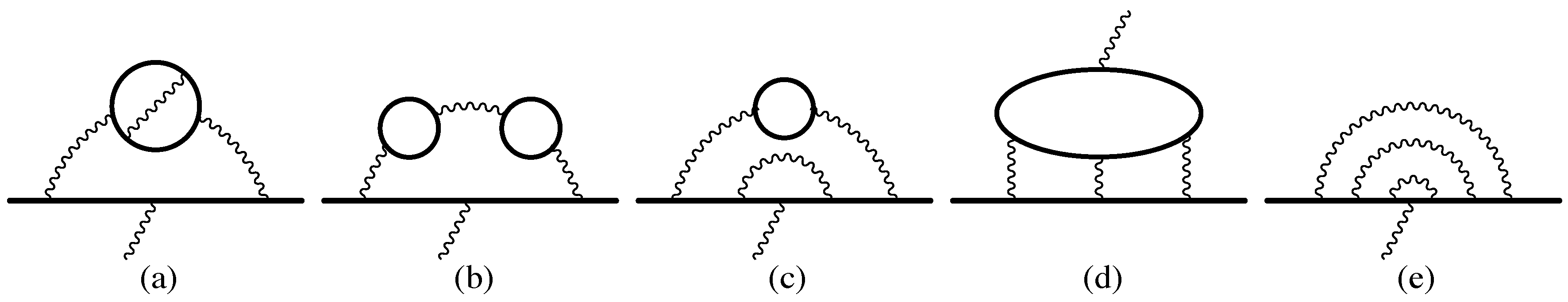
One of the recent achievements in the QED calculation is the near-analytic result of the eighth-order mass-independent term $A_1^{\left(8\right)}$ obtained by S. Laporta [26]. The Feynman integrals of the 891 eighth-order vertex diagrams are expressed in momentum space representation. They are decomposed into 334 master integrals (MI) according to the Laporta algorithm [36]. These MIs are numerically evaluated with high precision, up to 9600 digits, using the difference equation and/or the differential equation methods. The numerical values are then fitted by using the PSLQ algorithm [37,38], which is a finder of integer relations, and the analytic expressions of the MIs are determined. The MIs for the eighth-order cannot be expressed only by the elementary functions. They contain harmonic polylogarithms and one-dimensional integrals of the products of elliptic integrals. The analytic expressions of several MIs related to the internal light-by-light scattering diagrams, shown as IV(d) of Figure 4, have not been determined yet. Thus, the result obtained by S. Laporta is near-analytic, but known up to 1100 digits.

The tenth-order terms have been calculated only numerically thus far [35,39,40], though some small sets of diagrams are known analytically. An independent numerical double check has not been carried out yet. The mass-dependent term of the tenth-order was reported in [39]. The mass-independent term, $A_1^{\left(10\right)}$, has been calculated continuously on supercomputers even after some results were published in [40]. The latest numerical result

$$A_1^{\left(10\right)}=6.737\left(159\right)$$

(8)

is consistent with $6.675\left(192\right)$ given in Equation (16) of [40] and supersedes it.

Obviously, the mass-dependent terms $A_2$ and $A_3$ depend on the lepton-mass ratios provided by [41,42], and they are used as input parameters. However, they are the only input parameters of QED calculation. Notably, the mass-independent contribution $A_1$ is calculated without any input parameters. Principles, such as $U\left(1\right)$ gauge theory, Lorentz and CPT symmetries, and renormalizability determine $A_1$ completely.

In order to obtain the theoretical prediction of $a_e$, however, we need the input parameter determined from measurements of the nature. QED itself cannot determine what the fine-structure constant $\alpha$ is. Its value can only be derived from measurements. The quantum Hall resistance, which is named as the von Klitzing constant $R_K=h/e^2$, used to be the best method to determine the value of $\alpha$. However, the current best is to use atomic recoil measurements. A quotient of the Planck constant and the mass of an atom X, $h/m_X$, can be precisely determined by using atom interferometry [44]. Two quantum states of an atom are spatially separated by transferring momenta through Bloch oscillation of the optical lattice made of laser beams [45]. The obtained quotient is converted to $\alpha$ through

$$\alpha \left(X\right)={\left[\frac{2R_{\infty }}{c}\frac{A_r\left(X\right)}{A_r\left(e\right)}\frac{h}{m_X}\right]}^{1/2},$$

(9)

where $R_{\infty }$ is the Rydberg constant and $A_r\left(X\right)$ and $A_r\left(e\right)$ are the relative atomic masses of an atom X and an electron, respectively, which is defined by $m_X/u$ ($m_e/u$), u being the unified atomic mass unit. All three are precisely known and found in the CODATA 2014 adjustment [41]. $A_r\left(X\right)$ is determined from the cyclotron frequency of an ion in the constant magnetic field. $A_r\left(e\right)$ is from the bound g factor of the electron, and $R_{\infty }$ is from hydrogen spectroscopy. To determine the values $A_r\left(e\right)$ and $R_{\infty }$ from the measured quantities, one needs the QED corrections that have been obtained from many theoretical calculations [41]. In this sense, the value of $\alpha \left(X\right)$ determined from the quotient $h/m_X$ is not perfectly independent of QED. However, the uncertainties due to QED corrections are sufficiently small, and the uncertainty from the quotient $h/m_X$ dominates over others. Therefore, $\alpha \left(X\right)$ can be regarded as an independent determination of QED.

Recently, two new measurements on the hydrogen spectra have been carried out, and new values of $R_{\infty }$ have been reported. One is the 2S–4P transition by A. Beyer et al. [46]. Their $R_{\infty }$ is different from the CODATA adjusted value by 3.3$\sigma$. Another is the 1S–3S transition by H. Fleurbaey et al., which reports a value of $R_{\infty }$ consistent with CODATA [47]. If we use the value of $R_{\infty }$ from [46], it increases the value of ${\alpha }^{-1}$ by only $0.3\times {10}^{-8}$, which is within the uncertainty of $\alpha$ due to the $h/m_X$ measurements. Thus, we use the CODATA2014 adjustment value for $R_{\infty }$. The values of $\alpha$ currently available are from the Rb atom [48] and Cs atom [49] measurements of $h/m_X$ and are obtained as

$$\begin{array}{cc}\hfill {\alpha }^{-1}\left(\mathrm{Rb}\right)=& 137.035998995\left(85\right),\hfill \end{array}$$

(10)

$$\begin{array}{cc}\hfill {\alpha }^{-1}\left(\mathrm{Cs}\right)=& 137.035999046\left(27\right).\hfill \end{array}$$

(11)

Using them and hadronic and weak contributions to $a_e$ as listed in

Table 2. Standard model contributions to the electron anomalous magnetic moment $a_e$ in units of ${10}^{-12}$. The second-, fourth-, sixth-, and eighth-order mass-independent contributions of QED are evaluated with two values of the fine-structure constant: the upper and lower numbers are determined with $\alpha \left(\mathrm{Rb}\right)$ of the Rb atom recoil and $\alpha \left(\mathrm{Cs}\right)$ of the Cs atom recoil measurements, respectively. The difference of two values of $\alpha$ does not affect other QED contributions, weak or hadronic contributions. The weak and hadronic contributions are quoted from [22]. The hadronic contribution is further divided into the leading-order (LO) vacuum-polarization (VP) contribution, the next-to-leading-order (NLO) VP contiribution, the next-to-next-to-leading-order (NNLO) VP contribution, and the light-by-light scattering (LbyL) contribution.

QED	Mass-Independent	Mass-Dependent	Sum
2nd	1 161 409 733.64 (72)	0	1 161 409 733.63 (72)
	1 161 409 733.21 (23)		1 161 409 733.21 (23)
4th	−1 772 305.0652 (22)	2.814 1613 (13)	−1 772 302.2510 (22)
	−1 772 305.063 85 (70)		−1 772 302.249 69 (70)
6th	14 804.203 691 (28)	−0.093 240 76 (10)	14 804.110 450 (28)
	14 804.203 6740 (88)		14 804.110 4333 (88)
8th	−55.667 989 46 (14)	0.026 909 719 (35)	−55.641 079 74 (14)
	−55.667 989 379 (44)		−55.641 079 660 (56)
10th	0.456 (11)	−0.000 258 (26)	0.455 (11)
$a_e\left(\mathrm{QED}\right)$	1 159 652 177.57 (72)	2.747 5720 (14)	1 159 652 180.31 (72)
	1 159 652 177.14 (23)		1 159 652 179.88 (23)
$a_e\left(\mathrm{weak}\right)$			0.030 53 (23)
hadron LO VP			1.849 (10)
NLO VP			−0.2213 (11)
NNLO VP			0.027 99 (17)
LbyL			0.037 (5)
$a_e\left(\mathrm{hadron}\right)$			1.693 (12)
$a_e$			1 159 652 182.04 (72)
			1 159 652 181.61 (23)

, we obtain the theoretical prediction of $a_e$ as

$$\begin{array}{cc}\hfill a_e(\mathrm{theory}:\alpha \left(\mathrm{Rb}\right))=& 1159652182.037\left(720\right)\left(11\right)\left(12\right)\times {10}^{-12},\hfill \end{array}$$

(12)

$$\begin{array}{cc}\hfill a_e(\mathrm{theory}:\alpha \left(\mathrm{Cs}\right))=& 1159652181.606\left(229\right)\left(11\right)\left(12\right)\times {10}^{-12},\hfill \end{array}$$

(13)

where the uncertainties are due to the fine-structure constant $\alpha$, numerical evaluation of the tenth-order QED, and the hadronic contribution in this order. Note that the uncertainty of QED is now smaller than that of hadrons.

The best measurement of $a_e$ was performed at Harvard. Their result was [50]

$$a_e\left(\mathrm{expt}.\right)=1159652180.73\left(28\right)\times {10}^{-12}.$$

(14)

The differences between theory and measurement are

$$\begin{array}{cc}\hfill a_e(\mathrm{theory}:\alpha \left(\mathrm{Rb}\right))-a_e\left(\mathrm{expt}.\right)=& 1.31\left(77\right)\times {10}^{-12},\hfill \end{array}$$

(15)

$$\begin{array}{cc}\hfill a_e(\mathrm{theory}:\alpha \left(\mathrm{Cs}\right))-a_e\left(\mathrm{expt}.\right)=& 0.88\left(36\right)\times {10}^{-12},\hfill \end{array}$$

(16)

where the discrepancies are about 1.7$\sigma$ and 2.4$\sigma$ for $\alpha \left(\mathrm{Rb}\right)$ and $\alpha \left(\mathrm{Cs}\right)$, respectively.

We can obtain one more value of $\alpha$ recalling that the theory of $a_e$ depends almost exclusively on $\alpha$. Equating the theoretical formula of $a_e$ (3) with the measurement (14), we obtain

$${\alpha }^{-1}\left(a_e\right)=137.0359991496\left(13\right)\left(14\right)\left(330\right),$$

(17)

where the uncertainties are from the numerical evaluation of the tenth-order QED term, the hadronic contribution, and the measurement (14). The differences in $\alpha$ from the atomic recoil determinations are

$$\begin{array}{c}\hfill {\alpha }^{-1}\left(a_e\right)-{\alpha }^{-1}\left(\mathrm{Rb}\right)=0.155\left(91\right)\times {10}^{-6},\end{array}$$

(18)

$$\begin{array}{c}\hfill {\alpha }^{-1}\left(a_e\right)-{\alpha }^{-1}\left(\mathrm{Cs}\right)=0.104\left(43\right)\times {10}^{-6},\end{array}$$

(19)

where the discrepancies are about 1.7$\sigma$ and 2.4$\sigma$ for $\alpha \left(\mathrm{Rb}\right)$ and $\alpha \left(\mathrm{Cs}\right)$, respectively.

3. Preliminary Steps to QED Loop Calculation

3.1. QED Scattering Amplitude

In order to investigate the magnetic property of a single electron, let us consider the scattering of an electron by an external magnetic field. QED respects symmetries such as Lorentz, charge, parity, and time-reversal symmetries. Therefore, the scattering amplitude of an electron by an external photon field should be expressed only by two form factors $F_1$ and $F_2$:

$$e\overline{u}\left(p_{\mathrm{out}}\right)\left[{\gamma }^{\mu }{F}_1\left(q^2\right)+\frac{i}{2m}{\sigma }^{\mu \nu }{q}_{\nu }{F}_2\left(q^2\right)\right]u\left(p_{\mathrm{in}}\right)A_{\mu }^{\mathrm{ext}}\left(q^2\right),$$

(20)

where ${\sigma }^{\mu \nu }=\frac{i}{2}({\gamma }^{\mu }{\gamma }^{\nu }-{\gamma }^{\nu }{\gamma }^{\mu })$ and the external electron momenta are on-the-mass-shell:

$$p_{\mathrm{in}}^2={\left(p-\frac{q}{2}\right)}^2=m^2,p_{\mathrm{out}}^2={\left(p+\frac{q}{2}\right)}^2=m^2,q^2<0.$$

(21)

$F_1\left(q^2\right)$ and $F_2\left(q^2\right)$ are called charge (or Dirac) and magnetic (or Pauli) form factors, respectively.

If we follow the on-shell renormalization scheme so that the electron charge e is the very elementary charge observed in any non-relativistic systems, the charge form factor should be renormalized as

$$F_1\left(0\right)=1.$$

(22)

On the other hand, there is no reason that $F_2\left(0\right)$ should disappear. In fact, a non-vanishing value $F_2\left(0\right)$ gives rise to an anomalous magnetic moment of the electron.

Substituting the Gordon identity

$$\overline{u}\left(p_{\mathrm{out}}\right){\gamma }^{\mu }u\left(p_{\mathrm{in}}\right)=\frac{1}{2m}\overline{u}\left(p_{\mathrm{out}}\right)\{p^{\mu }+i{\sigma }^{\mu \nu }{q}_{\nu }\}u\left(p_{\mathrm{in}}\right)$$

(23)

into (20), we can rewrite the scattering amplitude as

$$e\overline{u}\left(p_{\mathrm{out}}\right)\left[\frac{p^{\mu }}{2m}{F}_1\left(q^2\right)+\frac{i}{2m}{\sigma }^{\mu \nu }{q}_{\nu }\{F_1\left(q^2\right)+F_2\left(q^2\right)\}\right]u\left(p_{\mathrm{in}}\right)A_{\mu }^{\mathrm{ext}}\left(q^2\right).$$

(24)

In the non-relativistic limit and static limit of $q\to 0$, only ${\sigma }^{ij},i,j=1,2,3$ contributes, and the second term of (24) is reduced to

$$-\frac{e}{2m}(1+F_2\left(0\right)){\psi }^{†}\overrightarrow{\sigma }·\overrightarrow{B}\psi ,$$

(25)

where $\psi$ is a two-component spinor and ${\sigma }^i$ is the Pauli matrix. The effective Hamiltonian of the interaction between a magnetic moment $\overrightarrow{\mu }$ and an external static magnetic field $\overrightarrow{B}$ is

$$\widehat{H}=-\overrightarrow{\mu }·\overrightarrow{B},\overrightarrow{\mu }\equiv g\frac{e}{2m}\overrightarrow{s},$$

(26)

where $\overrightarrow{s}=\overrightarrow{\sigma }/2$ is the spin of the electron. We can therefore identify the spin g-factor of the electron as

$$g=2(1+F_2\left(0\right)),\mathrm{or}{a}_e\equiv \frac{g-2}{2}=F_2\left(0\right).$$

(27)

Thus far, no successful explanation has been given for why the anomalous magnetic moment $a_e=F_2\left(0\right)$ should be positive. We know that $a_e$ is positive because Schwinger’s calculation of the one-loop Feynman diagram of QED turns out to be $+1/2$ as a coefficient of $\alpha /\pi$.

3.2. Feynman Diagrams

In order to compute $a_e$, we need to evaluate the scattering amplitude of the electron within the framework of QED perturbation theory. It is the scattering amplitude that we want to compute, so quantum corrections on external electron legs must be taken into account. However, if covariant gauge fixing for the photon field is chosen, self-energy corrections on external electron legs provide no effect after renormalization with the on-shell condition. Since we use the Feynman gauge for the photon field with the on-shell renormalization condition, it is sufficient for us to deal with one-particle irreducible (1PI) vertex diagrams. If a non-covariant gauge, such as the Coulomb gauge, is chosen, quantum corrections on external legs must be taken into account to compute $a_e$ [51].

The number of 1PI-vertex-Feynman diagrams of a given order of perturbation theory can be counted by using QED in zero-dimensional space and time [52,53]. In zero dimensions, the photon and electron fields are just bosonic and fermionic numbers, respectively, and the path-integral over field variables can be exactly performed. Assume that QED consists of electrons and photons only. The generating function $\mathsf{\Gamma }$ for the 1PI-vertex Green function is analytically calculable, and its closed form expressed by a modified Bessel function is given in [53]. Its series expansion in the coupling constant e is found as

$$\mathsf{\Gamma }=1+e^2+7e^4+72e^6+891e^8+12672e^{10}+202770e^{12}+3602880e^{14}+\cdots .$$

(28)

The coefficient of the $2n\mathrm{th}$ power of e is the number of 1PI-vertex diagrams of the $2n\mathrm{th}$-order perturbation theory of QED. Typical vertex Feynman diagrams of the second-, fourth-, sixth-, eighth-, and tenth-orders of the perturbation theory are shown in Figure 1, Figure 2, Figure 3, Figure 4 and Figure 5, respectively.

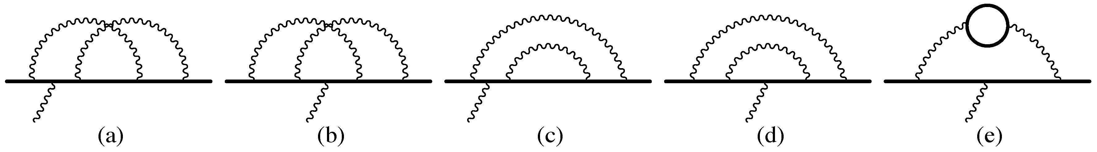
There are three main structures of these Feynman diagrams. One type is a diagram without an electron loop such as (e) in Figure 3, Group V in Figure 4, and Set V in Figure 5. The second type is a diagram with electron loops, but only of the vacuum-polarization (VP) type, such as (a)–(c) in Figure 3, Group I(a–d), II(a–c), III in Figure 4. The third type is a diagram including an electron loop to which four or more photons are externally attached. They, light-by-light scattering (LbyL) diagrams, appear for the first time in the sixth-order perturbation theory, as shown in (d) in Figure 3. The tenth-order diagram I(j) shown in Figure 5 contains a VP function consisting of two LbyL loops. This is classified as belonging to the VP type.

The computational difficulty of diagrams (of the same order) depends very much on their structures. Once the integral of a diagram without a fermion loop is constructed, insertion of VP functions is almost trivial, particularly when a VP is the second- or fourth-order VP function, which are known as compact and analytic forms. For the sixth-order and higher order VP functions, their construction based on Feynman diagrams is relatively easy. Since VP functions consist of closed loop diagrams, they are free from infrared (IR) divergence and suffer only from ultraviolet (UV) divergence. This is because IR divergence of a QED Feynman diagram occurs only when a massless photon is attached to on-shell electron lines. This never happens in a VP Feynman diagram. Numerical handling of UV divergences is much easier, especially for our recipe called the $\mathbb{K}$-operation, than those of IR divergences. Furthermore, the Padé approximants for the sixth- and eighth-order vacuum-polarization functions consisting of a single fermion loop are available [54,55]. They allow us to do an independent and rigorous check of the contributions involving the higher order VP functions.

Vertex diagrams including an LbyL loop start to appear in the sixth-order. This means that diagrams involving an LbyL loop have a simple structure of UV divergence. It is known that the Feynman integral of an LbyL diagram is particularly lengthy and complicated, and its analytic evaluation is very tough [6,26,56]. Numerical calculation of them, however, does not face such problems at all. The simple divergence structure makes construction of the integral comparatively easy and convergence of numerical integration fast.

The most challenging is thus the computation of higher order diagrams without a fermion loop. In the remaining sections, we will discuss how to numerically calculate them. Other diagrams with fermion loops will be discussed elsewhere.

4. QED Diagrams without a Fermion Loop

4.1. Ward–Takahashi Sum

Let us focus on QED vertex diagrams without a fermion loop. For the higher order terms of the perturbation theory, the number of Feynman diagrams grows factorially with the loop order [52]. Furthermore, as the order increases, the complexity of the integral derived from a Feynman diagram drastically increases. Reduction of the number of diagrams, if possible, is thus highly desirable. To achieve this goal, we combine vertex diagrams sharing the same quantum corrections and relate them to a self-energy diagram through the Ward–Takahashi identity:

$$q_{\mu }{\mathsf{\Lambda }}^{\mu }(p,q)=-\Sigma (p+\frac{q}{2})+\Sigma (p-\frac{q}{2}),$$

(29)

where ${\mathsf{\Lambda }}^{\mu }(p,q)$ is the “sum” of vertex diagrams that are obtained by inserting an external photon vertex in a fermion line of the self-energy diagram $\Sigma$ in every possible way. Differentiating both sides with respect to $q^{\nu }$ and taking a vanishing momentum transfer limit $q\to 0$, we obtain

$${\mathsf{\Lambda }}^{\nu }(p,q)=-q^{\mu }{\left[\frac{\partial {\mathsf{\Lambda }}_{\mu }(p,q)}{\partial q_{\nu }}\right]}_{q=0}-\frac{\partial \Sigma \left(p\right)}{\partial p_{\nu }}+\mathcal{O}\left(q^2\right).$$

(30)

This equation enables us to obtain the magnetic moment amplitude of the $2n\mathrm{th}$-order diagram by projecting it out from the right-hand side of (30). Although they are not explicitly written, photon momenta are imposed on a cut-off $\mathsf{\Lambda }$, and a small mass $\lambda$ is given to a photon. These regularization parameters are safely removed after the finite amplitude is constructed.

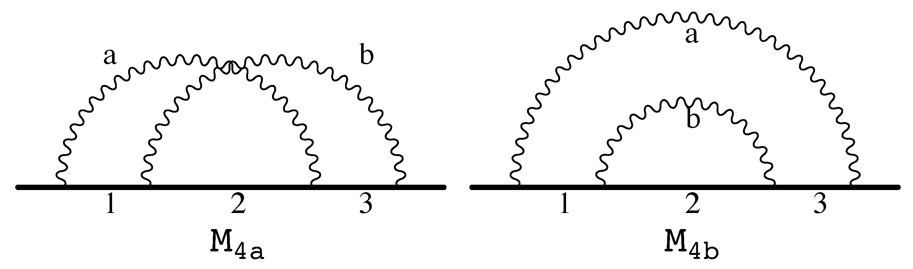
The QED Feynman–Dyson rules introduced in many QED textbooks lead to a Feynman integral expressed in momentum space. Instead, we use the parametric Feynman–Dyson rules [7,9,10] that enable us to write down the Feynman integral in terms of Feynman parameters without referring to the momentum representation at all. The Feynman integral derived from a $2n\mathrm{th}$-order self-energy diagram can be expressed using Feynman parameters: $z_1,z_2\cdots$ and $z_a,z_b,\cdots$ are assigned from the left to the right to $2n-1$ electron and n photon propagators, respectively. All Feynman parameters are non-negative, and the sum of all is restricted to one. As an example, two self-energy-like diagrams of the fourth-order are shown in Figure 6.

To illustrate the parametric Feynman–Dyson rules, we start with the Feynman–Dyson integral of the self-energy diagram $M_{4a}$ of the left pane of Figure 6:

$$\begin{array}{c}-i{\Sigma }_{4a}\left(p\right)={(-ie)}^4\int \frac{d^4{q}_1}{{\left(2\pi \right)}^4}\frac{d^4{q}_2}{{\left(2\pi \right)}^4}\frac{-i}{q_1^2-{\lambda }^2+iϵ}\frac{-i}{q_2^2-{\lambda }^2+iϵ}\hfill \\ \hfill {\gamma }^{\alpha }\frac{i({𝓅}_1+m)}{p_1^2-m^2+iϵ}{\gamma }^{\beta }\frac{i({𝓅}_2+m)}{p_2^2-m^2+iϵ}{\gamma }_{\alpha }\frac{i({𝓅}_3+m)}{p_3^2-m^2+iϵ}{\gamma }_{\beta },\end{array}$$

(31)

where $q_1$ and $q_2$ are the momenta of photon propagators a and b, respectively, and $p_1=p+q_1,p_2=p+q_1+q_2,p_3=p+q_2$ are the momenta flowing on the electron propagators 1, 2, and 3. By introducing the Feynman parameters $z_1,z_2,\cdots$ and using the trick

$$\frac{1}{X_1{X}_2\dots X_k}=(k-1)!{\int }_0^{1}d{z}_1{\int }_0^{1}d{z}_2\cdots {\int }_0^{1}d{z}_k\frac{\delta (1-z_1-z_2-\cdots -z_k)}{{(z_1{X}_1+z_2{X}_2+\cdots +z_k{X}_k)}^k},$$

(32)

the denominators of all propagators are combined as

$$z_a(q_1^2-{\lambda }^2)+z_b(q_2^2-{\lambda }^2)+z_1(p_1^2-m^2)+z_2(p_2^2-m^2)+z_3(p_3^2-m^2).$$

(33)

The loop momenta $q_1$ and $q_2$ can be “diagonalized”, and Equation (33) is rewritten as

$$z_{12a}{\left(q_1^d\right)}^2+\frac{U}{z_{12a}}{\left(q_2^d\right)}^2-V,V\equiv z_{ab}{\lambda }^2+z_{123}{m}^2-G{p}^2,$$

(34)

where $z_{ij\cdots }=z_i+z_j+\cdots$ and

$$\begin{array}{c}{q}_1^d=q_1+(z_{12}p+z_2{q}_2)/z_{12a},q_2^d=q_2+(z_{23}{z}_{12a}-z_{12}{z}_2)p/U,\hfill \\ U=z_{12a}{z}_{23b}-{\left(z_2\right)}^2,G=z_{123}-(z_{12a}{z}_{23}^2-2z_{12}{z}_2{z}_{23}+z_{23b}{z}_{12}^2)/U.\hfill \end{array}$$

(35)

The U function is a “Jacobian” from the momentum space to the Feynman parameter space. After the shift of the loop momenta, the numerator of the integrand of (31), $\mathbf{F}$, is expressed as

$$\mathbf{F}={\gamma }^{\alpha }({𝓀}_1+A_1𝓅+m){\gamma }^{\beta }({𝓀}_2+A_2𝓅+m){\gamma }_{\alpha }({𝓀}_3+A_3𝓅+m){\gamma }_{\beta },$$

(36)

where $k_i$’s are the linear combinations of the diagonalized loop momenta $q_1^d$ and $q_2^d$ and $A_i$’s are functions of Feynman parameters. Because of its definition in (34), G is obviously related to $A_i$ as

$$G=z_1{A}_1+z_2{A}_2+z_3{A}_3.$$

(37)

More systematic derivation of U and other functions of the Feynman parameters will be given in Section 4.3, which is based on graph theory and is easily applicable to any higher order diagrams.

The right-hand side of (30) for any order of the perturbation theory can be obtained by performing several manipulations on the Feynman parametric representation of a self-energy diagram $\mathcal{G}$. They are expressed as

$$\begin{array}{c}-q_{\mu }{\left[\frac{\partial {\mathsf{\Lambda }}^{\mu }(p,q)}{\partial q_{\nu }}\right]}_{q=0}={\left(\frac{-\alpha }{4\pi }\right)}^n(n-1)!q_{\mu }\int {\left(dz\right)}_{\mathcal{G}}\left({\mathbf{Z}}^{\mu \nu }\frac{1}{U^2{V}^n}+{\mathbf{C}}^{\mu \nu }\frac{1}{(n-1)U^2{V}^{n-1}}\right),\end{array}$$

(38)

$$\begin{array}{c}-\frac{\partial \Sigma \left(p\right)}{\partial p_{\nu }}={\left(\frac{-\alpha }{4\pi }\right)}^n(n-1)!\int {\left(dz\right)}_{\mathcal{G}}\left({\mathbf{N}}^{\nu }\frac{1}{U^2{V}^n}+{\mathbf{E}}^{\nu }\frac{1}{(n-1)U^2{V}^{n-1}}\right),\end{array}$$

(39)

where ${\left(dz\right)}_{\mathcal{G}}$ stands for integration variables over Feynman parameters subject to the constraint ${\sum }_i{z}_i=1$. The function U is a “Jacobian” for transformation from the momentum space to Feynman parametric space and V is the combined denominators of all propagators of the diagram $\mathcal{G}$. Explicit expressions of U and V will be determined later. The exact manipulations are given in [7,9,10]. Briefly speaking, the procedure corresponding to the operator ${\mathbf{Z}}^{\mu \nu }$ is to insert an external photon vertex to one of the electron propagators of a self-energy diagram and to differentiate this electron propagator with respect to the momentum q flowing in through the external photon vertex. The procedure corresponding to the operator ${\mathbf{C}}^{\mu \nu }$ is to insert an external photon vertex to one of the electron propagators and to differentiate with respect to q all other electron propagators to which an external photon vertex is not attached. The procedure corresponding to the operator ${\mathbf{N}}^{\nu }$ comes from the differentiation of the denominator function V with respect to $p_{\nu }$. The operator ${\mathbf{E}}^{\nu }$ is defined by ${\mathbf{E}}^{\nu }=\partial \mathbf{F}/\partial p_{\nu }$, where $\mathbf{F}$ is the product of all numerators of the electron propagators of a self-energy diagram.

The procedures and their corresponding operators of $\gamma$-matrices are explicitly constructed for the self-energy diagram $M_{4a}$. There are three electron propagators in which an external photon vertex can be inserted. Thus, the ${\mathbf{Z}}^{\mu \nu }$-operator consists of three terms:

$${\mathbf{Z}}^{\mu \nu }=z_1{\mathbf{Z}}_1^{\mu \nu }+z_2{\mathbf{Z}}_2^{\mu \nu }+z_3{\mathbf{Z}}_3^{\mu \nu },$$

(40)

where ${\mathbf{Z}}_i^{\mu \nu }$ is obtained by replacing the electron line factor ${\mathbf{l}}_i\equiv {𝓀}_i+A_i𝓅+m$ of $\mathbf{F}$ in (36) by ${\mathbf{S}}_i^{\mu \nu }$:

$${\mathbf{l}}_i⟶{\mathbf{S}}_i^{\mu \nu }\equiv \frac{1}{2}({\gamma }^{\mu }{\gamma }^{\nu }{\mathbf{l}}_i-{\mathbf{l}}_i{\gamma }^{\nu }{\gamma }^{\mu }).$$

(41)

${\mathbf{C}}^{\mu \nu }$ is constructed by picking up two electron line factors:

$${\mathbf{C}}^{\mu \nu }=C_{12}{\mathbf{F}}_{12}^{\mu \nu }+C_{13}{\mathbf{F}}_{13}^{\mu \nu }+C_{23}{\mathbf{F}}_{23}^{\mu \nu },$$

(42)

where ${\mathbf{F}}_{ij}^{\mu \nu }\mathrm{for}i<j$ can be obtained by replacing ${\mathbf{l}}_i$ and ${\mathbf{l}}_j$ of $\mathbf{F}$ by ${\gamma }^{\mu }$ and ${\gamma }^{\nu }$, respectively. The coefficient $C_{ij}\mathrm{for}i<j$ is defined in terms of $B_{ij}$, which will be defined later in Section 4.3, as

$$C_{ij}=\frac{1}{U^2}\sum _{k=1}^2\sum _{l=k+1}^3{z}_k{z}_l(B_{ik}^{\prime }{B}_{jl}^{\prime }-B_{il}^{\prime }{B}_{jk}^{\prime }),$$

(43)

where

$$B_{ij}^{\prime }=B_{ij}-{\delta }_{ij}\frac{U}{z_i}.$$

(44)

Since the denominator function V contains the external momentum p as given in (34), the ${\mathbf{N}}^{\nu }$-operator is trivially determined as

$${\mathbf{N}}^{\nu }=2p^{\nu }G\mathbf{F},$$

(45)

where G is defined in (34), and its explicit form is given in (37). The explicit form of ${\mathbf{E}}^{\nu }$-operator for $M_{4a}$ is given by

$${\mathbf{E}}^{\nu }=A_1{\mathbf{F}}_1^{\nu }+A_2{\mathbf{F}}_2^{\nu }+A_3{\mathbf{F}}_3^{\nu },$$

(46)

where ${\mathbf{F}}_i$ is obtained by replacing ${\mathbf{l}}_i$ of $\mathbf{F}$ by ${\gamma }^{\nu }$.

4.2. Projection of Anomaly Contributions

We are now ready to extract the anomalous magnetic moment contribution paying attention to its Lorentz structure. After projection operators are applied to (38) and (39), the magnetic moment amplitude has the form of

$$M_{\mathcal{G}}^{\left(2n\right)}={\left(-\frac{\alpha }{4\pi }\right)}^n(n-1)!\int \frac{{\left(dz\right)}_{\mathcal{G}}}{U^2}\left\{\frac{1}{n-1}\frac{\mathbf{E}+\mathbf{C}}{V^{n-1}}+\frac{\mathbf{N}+\mathbf{Z}}{V^n}\right\},$$

(47)

where the functions $\mathbf{E}$, $\mathbf{C}$, $\mathbf{N}$, $\mathbf{Z}$ are defined as

$$\begin{array}{cccc}\hfill \mathbf{N}& =\frac{1}{4}\mathrm{Tr}\left[P_1^{\nu }{\mathbf{N}}_{\nu }\right],\hfill & \hfill \mathbf{E}& =\frac{1}{4}\mathrm{Tr}\left[P_1^{\nu }{\mathbf{E}}_{\nu }\right],\hfill \\ \hfill \mathbf{C}& =\frac{1}{4}\mathrm{Tr}\left[P_2^{\mu \nu }{\mathbf{C}}_{\mu \nu }\right],\hfill & \hfill \mathbf{Z}& =\frac{1}{4}\mathrm{Tr}\left[P_2^{\mu \nu }{\mathbf{Z}}_{\mu \nu }\right],\hfill \end{array}$$

(48)

and the projection operators of $P_1$ and $P_2$ are given by

$$\begin{array}{c}{P}_1^{\nu }=\frac{1}{3}{\gamma }^{\nu }-\left(1+\frac{4}{3}𝓅\right)p^{\nu },\\ P_2^{\mu \nu }=\frac{1}{3}(𝓅+1)(g^{\mu \nu }-{\gamma }^{\mu }{\gamma }^{\nu }+p^{\mu }{\gamma }^{\nu }-p^{\nu }{\gamma }^{\mu })\end{array}$$

(49)

with $m^2=p^2=1$. Hereafter, we set $m^2=p^2=1$ and the photon mass $\lambda =0$, unless we need to distinguish $m^2$ and $p^2$.

4.3. Building Blocks $B_{ij}$

We introduce the “correlation” functions $B_{ij}$ between two propagators i and j of the same diagram. The propagators i and j can be any of the electron or photon propagators. These $B_{ij}$’s are the very basic building blocks of the Feynman parametric representation of a loop diagram. They are determined by and only by the topology of a loop diagram [57,58].

Let us introduce a chain diagram that is obtained when the external legs of a diagram are removed and no distinction is made between electron and photon propagators. Thus, chain diagrams of each order of the QED perturbation theory are identical to those of the scalar ${\varphi }^3$ theory. A line between two nodes of a chain diagram is associated with a sum of several Feynman parameters belonging to it, and its direction is freely assigned. For a given chain diagram with n loops with $n>1$, the numbers of nodes and lines are $2(n-1)$ and $3(n-1)$, respectively. For $n=1$, a chain diagram has no node, and it is just a circle. The number of topologically-distinguished chain diagrams at a given order of perturbation theory is quite small compared with those of Feynman diagrams. They are 1, 1, 2, 5, and 16 for the second-, fourth-, sixth-, eighth-, and tenth-order perturbation theory of QED.

A given n loop chain diagram has n independent closed circuits. In the case of a QED self-energy diagram without a fermion loop, independent closed circuits are easily identified. A closed circuit consists of a photon propagator and electron propagators that lie between the two vertices where this photon comes in and out. The direction of a closed circuit is chosen as the same as that of the electron propagators.

The diagrams $M_{4a}$ and $M_{4b}$ are reduced to the same chain diagram. For $M_{4a}$, the independent closed circuits $c_1$ and c${}_2$ consist of two lines $l_1=z_1+z_a$ and $l_2=z_2$ and two lines $l_2=z_2$ and $l_3=z_3+z_b$, respectively. For $M_{4b}$, the independent circuits $c_1$ and $c_2$ consist of two lines $l_1=z_1+z_3+z_a$ and $l_2=z_2$ and two lines $l_2=z_2$ and $l_3=z_b$, respectively.

The $n\times 3(n-1)$ loop matrix ${\mathbf{T}}_{i\beta }$ for a chain diagram is defined as follows:

$${\mathbf{T}}_{i\beta }=\left\{\begin{array}{cc}\hfill +1& \mathrm{if}\mathrm{the}\mathrm{line}\beta \mathrm{is}\mathrm{contained}\mathrm{in}\mathrm{the}\mathrm{circuit}{c}_i\mathrm{and}\mathrm{has}\mathrm{the}\mathrm{same}\mathrm{direction}\mathrm{of}{c}_i,\hfill \\ \hfill -1& \mathrm{if}\mathrm{the}\mathrm{line}\beta \mathrm{is}\mathrm{contained}\mathrm{in}\mathrm{the}\mathrm{circuit}{c}_i\mathrm{and}\mathrm{has}\mathrm{the}\mathrm{opposite}\mathrm{direction}\mathrm{of}{c}_i,\hfill \\ \hfill 0& \mathrm{if}\mathrm{the}\mathrm{line}\beta \mathrm{is}\mathrm{not}\mathrm{contained}\mathrm{in}\mathrm{the}\mathrm{circuit}{c}_i,\hfill \end{array}\right.$$

(50)

where i indicates one of the independent chain circuits and $\beta$ stands for a line number. The loop matrix ${\mathbf{T}}_{i\beta }$ for $M_{4a}$ is

$$\left(\begin{array}{ccc}+1& +1& 0\\ 0& +1& +1\end{array}\right)$$

(51)

and the same for $M_{4b}$. The $n\times n$ symmetric matrix ${\mathbf{U}}_{ij}$ is derived from ${\mathbf{T}}_{i\beta }$ such that

$${\mathbf{U}}_{ij}=\sum _{\beta =1}^{3(n-1)}{\mathbf{T}}_{i\beta }{\mathbf{T}}_{j\beta }{l}_{\beta }.$$

(52)

The Jacobian U in (38) and (39) is obtained as the determinant of the matrix ${\mathbf{U}}_{ij}$:

$$U\equiv det\left({\mathbf{U}}_{ij}\right).$$

(53)

The correlation function $B_{\alpha \beta }$ between two lines $l_{\alpha }$ and $l_{\beta }$ of a chain diagram is defined by

$$B_{\alpha \beta }=\sum _{k=1}^n\sum _{l=1}^n{\mathbf{U}}_{kl}^{-1}{\mathbf{T}}_{k\alpha }{\mathbf{T}}_{l\beta }U,$$

(54)

where ${\mathbf{U}}_{kl}^{-1}$ is the inverse matrix of ${\mathbf{U}}_{ij}$.

The $B_{ij}$ between two propagators of a Feynman diagram is identical with $B_{\alpha \beta }$, where the propagator i and j are contained in the lines $\alpha$ and $\beta$, respectively. The scalar current $A_i$ of an electron propagator introduced in (36) is expressed using $B_{ij}$ as

$$A_i=1-\sum _{j=1}^{2n-1}{z}_j{B}_{ij}/U.$$

(55)

The denominator function V is given by

$$V=z_1+z_2+\cdots +z_{2n-1}-G,$$

(56)

where

$$G=z_1{A}_1+z_2{A}_2+\cdots +z_{2n-1}{A}_{2n-1}.$$

(57)

For $M_{4a}$, we find U, $B_{ij}=B_{ji}$ in terms of Feynman parameters as

$$\begin{array}{c}U=z_{1a}{z}_2+z_{1a}{z}_{3b}+z_2{z}_{3b},\hfill \end{array}$$

(58)

$$\begin{array}{c}{B}_{11}=z_2+z_{3b},B_{12}=z_{3b},B_{13}=-z_2,B_{22}=z_{3b}+z_{1a},B_{23}=z_{1a},B_{33}=z_{1a}+z_2,\hfill \end{array}$$

(59)

and for $M_{4b}$,

$$\begin{array}{c}U=z_{13a}{z}_2+z_{13a}{z}_b+z_2{z}_b,\hfill \end{array}$$

(60)

$$\begin{array}{c}{B}_{11}=B_{13}=B_{33}=z_2+z_b,B_{12}=B_{23}=z_b,B_{22}=z_b+z_{13a}.\hfill \end{array}$$

(61)

It is easy to check that U of (58) and G of (37) with (55) and (59) are identical to those given in (35).

Even for a higher order diagram, the construction of the loop matrix ${\mathbf{T}}_{i\beta }$ is trivial. Once the loop matrix is formed, the building blocks of the Feynman parametric representation can be obtained. For instance, the loop matrix ${\mathbf{T}}_{i\beta }$ of the tenth-order diagram $X_{253}$ of Figure 7 is found as

$$\left(\begin{array}{cccccccccccc}+1& +1& +1& +1& +1& +1& +1& +1& 0& 0& 0& 0\\ 0& +1& +1& +1& +1& +1& +1& +1& +1& 0& 0& 0\\ 0& 0& +1& 0& 0& 0& 0& 0& 0& +1& 0& 0\\ 0& 0& 0& 0& +1& +1& 0& 0& 0& 0& +1& 0\\ 0& 0& 0& 0& 0& +1& +1& 0& 0& 0& 0& +1\end{array}\right),$$

(62)

where the lines $l_{\beta }$ are chosen as

$$\begin{array}{c}{l}_1=z_{19a},l_2=z_2,l_3=z_3,l_4=z_4,l_5=z_5,l_6=z_6,\hfill \\ l_7=z_7,l_8=z_8,l_9=z_b,l_{10}=z_c,l_{11}=z_d,l_{12}=z_e,\hfill \end{array}$$

(63)

and the closed circuits are numbered according to the lexicographical order of the contained photon propagators. With this matrix, Formulas (52)–(57) and (43) lead to all necessary building blocks.

4.4. Integration over Loop Momenta

We perform integration over diagonalized loop momenta. In our formulation, this can be done by two steps, by which the loop momenta $k_i$ appearing in (36) should turn into “contractions”.

Firstly, all $k_i$’s in the numerator are replaced by the correlation functions. If a term of the numerator contains an odd number of $k_i$’s, it is dismissed after integration. Up to the sixth-order diagrams, the numerator contains 0, 2, or 4 $k_i$’s. Therefore, the contraction rules of two $k_i$’s needed are

$$\begin{array}{cc}\hfill p·k_{i1}p·k_{i2}p·k_{i3}p·k_{i4}& \Rightarrow {\left(p^2\right)}^2(B_{i1i2}{B}_{i3i4}+B_{i1i3}{B}_{i2i4}+B_{i1i4}{B}_{i2i3}),\hfill \\ \hfill p·k_{i1}p·k_{i2}{k}_{i3}·k_{i4}& \Rightarrow p^2(4B_{i1i2}{B}_{i3i4}+B_{i1i3}{B}_{i2i4}+B_{i1i4}{B}_{i2i3}),\hfill \\ \hfill k_{i1}·k_{i2}{k}_{i3}·k_{i4}& \Rightarrow 4(4B_{i1i2}{B}_{i3i4}+B_{i1i3}{B}_{i2i4}+B_{i1i4}{B}_{i2i3}),\hfill \\ \hfill p·k_{i1}p·k_{i2}& \Rightarrow p^2{B}_{i1i2}\hfill \\ \hfill k_{i1}·k_{i2}& \Rightarrow 4B_{i1i2},\hfill \end{array}$$

(64)

where the coefficient 4 represents the space-time dimension. The extension to the eighth- or tenth-order diagrams is straightforward.

Secondly, the powers of V are changed according to the number of contractions of $k_i$’s. As is seen in (47), the inverse power of V starts with either n or $n-1$. If the numerator originally contains $2m$$k_i$’s and is produced by m contractions of $k_i$’s, the denominators change from $V^n$ or $V^{n-1}$ to

$$\begin{array}{cc}\hfill V^n& \Rightarrow {(-2)}^m{U}^m{V}^{n-m}(n-1)(n-2)\cdots (n-m)\hfill \\ \hfill V^{n-1}& \Rightarrow {(-2)}^m{U}^m{V}^{n-1-m}(n-2)(n-3)\cdots (n-1-m).\hfill \end{array}$$

(65)

After applying the whole contraction procedures, the amplitude of the anomalous magnetic moment from the self-energy-like diagram $\mathcal{G}$ can be written in terms of the Feynman parameters as

$$\begin{array}{c}{M}_{\mathcal{G}}^{\left(2n\right)}={\left(\frac{-\alpha }{4\pi }\right)}^n(n-1)!\int \frac{{\left(dz\right)}_{\mathcal{G}}}{U^2}[\frac{1}{n-1}\left(\frac{E_0+C_0}{V^{n-1}}+\frac{E_1+C_1}{U{V}^{n-2}}+\cdots +\frac{E_{n-2}+C_{n-2}}{U^{n-2}V}\right)\hfill \\ \hfill +\left(\frac{N_0+Z_0}{V^n}+\frac{N_1+Z_1}{U{V}^{n-1}}+\cdots +\frac{N_{n-1}+Z_{n-1}}{U^{n-1}V}\right)].\end{array}$$

(66)

For $n=2$, the unrenormalized amplitude $M_{4a}$ thus has the form:

$$M_{4a}={\left(\frac{-\alpha }{4\pi }\right)}^2\int \frac{{\left(dz\right)}_{4a}}{U^2}\left[\frac{E_0+C_0}{V}+\frac{N_0+Z_0}{V^2}+\frac{N_1+Z_1}{UV}\right],$$

(67)

and the explicit forms of the numerator functions are found to be

$$\begin{array}{cc}\hfill E_0& =8(2A_1{A}_2{A}_3-A_1{A}_2-A_2{A}_3-A_3{A}_1),\hfill \\ \hfill C_0& =-24z_a{z}_b/U,\hfill \\ \hfill N_0& =G[E_0+8(2-A_1-A_2-A_3)],\hfill \\ \hfill Z_0& =8z_1(-A_1+A_2+A_3+A_1{A}_2+A_1{A}_3-A_2{A}_3)\hfill \\ & +8z_2(1-A_1{A}_2+A_1{A}_3-A_2{A}_3+2A_1{A}_2{A}_3)\hfill \\ & +8z_3(A_1+A_2-A_3-A_1{A}_2+A_1{A}_3+A_2{A}_3),\hfill \\ \hfill N_1& =8G[B_{12}(2-A_3)+2B_{13}(1-2A_2)+B_{23}(2-A_1)],\hfill \\ \hfill Z_1& =8z_1[B_{12}(A_3-1)-B_{13}-B_{23}{A}_1)]\hfill \\ & +8z_2[B_{12}(1-A_3)-4B_{13}{A}_2+B_{23}(1-A_1)]\hfill \\ & +8z_3[-B_{12}{A}_3-B_{13}+B_{23}(A_1-1)].\hfill \end{array}$$

(68)

For $M_{4b}$, the formal expression of the amplitude is the same as (67). Because $A_1=A_3,B_{12}=B_{23},$ $B_{11}=B_{33}$ for $M_{4b}$, the numerator functions are much shorter and are given by

$$\begin{array}{cc}\hfill E_0& =8A_1[4(A_2-A_1)-A_1{A}_2],\hfill \\ \hfill C_0& =-8A_2,\hfill \\ \hfill N_0& =-8G[4(1-A_1+A_1^2)+A_2(1-4A_1+A_1^2)],\hfill \\ \hfill Z_0& =8z_{13}[4A_1-A_2(1+A_1^2)]+8z_2{A}_2(1+A_1^2),\hfill \\ \hfill N_1& =8G[8(B_{11}-B_{12})+3A_1{B}_{12}],\hfill \\ \hfill Z_1& =24(z_{13}-z_2)A_1{B}_{12}.\hfill \end{array}$$

(69)

4.5. UV Renormalization by $\mathbb{K}$-Operation

Let us focus on the structure of UV divergence of an unrenormalized amplitude $M_{\mathcal{G}}^{\left(2n\right)}$. Though the amplitude $M_{\mathcal{G}}^{\left(2n\right)}$ originates from a self-energy diagram, it does not suffer from an overall divergence associated with this $2n\mathrm{th}$-order self-energy diagram. This is because its UV divergence is dropped when the anomalous magnetic moment contribution is projected out from it. UV divergences of $M_{\mathcal{G}}^{\left(2n\right)}$ come from subdiagrams of a self-energy diagram $\mathcal{G}$, either self-energy or vertex, of a lower order than the $2n\mathrm{th}$.

As is discussed in Section 3, the renormalization procedure we have to use is the on-shell renormalization condition. However, the on-shell renormalization is not suitable for numerical calculation of a Feynman integral. If we perform the on-shell renormalization for an unrenormalized amplitude, UV divergence can be canceled, but it brings new types of IR divergence into the integral. We, therefore, carry out the renormalization in two steps.

Our UV subtraction method is named as the $\mathbb{K}$-operation, which is realized in practice as a simple power-counting rule. The form of a UV subtraction term is picked up by applying the $\mathbb{K}$-operation to the unrenormalized amplitude of (66), which is expressed with the auxiliary functions U, V, $A_i$, $B_{ij}$, and $C_{ij}$. The $\mathbb{K}$-operation is also applied to these auxiliary functions. The resultant integral is written in the same Feynman parameter space of the unrenormalized amplitude, and point-wise UV subtraction is realized. With a little algebra on the Feynman parameters, the resultant integral for UV subtraction exactly decouples into the renormalization constant determined and the lower-order magnetic moment amplitude. This renormalization constant contains the same UV divergence of the on-shell renormalization constant, but it is free from IR divergence, unlike the on-shell one.

Let us examine the fourth-order cases. The diagram $M_{4a}$ has a second-order vertex subdiagram ${\mathcal{S}}_{12a}$ consisting of the electron propagators 1 and 2 and the photon propagator a. To extract the UV divergent terms associated with this subdiagram, the $\mathbb{K}(1,2)$-operation is applied to $M_{4a}$. The $\mathbb{K}(1,2)$-operation in the Feynman parametric space is equivalent to taking the simultaneous limit of vanishing Feynman parameters of $z_1$, $z_2$, and $z_a$, which form ${\mathcal{S}}_{12a}$.

The $\mathbb{K}(1,2)$-operation on $B_{ij}$ and U reflects the decoupling of subdiagram ${\mathcal{S}}_{12a}$ and residual diagram ${\mathcal{G}}_{3b}^{\prime }\equiv \mathcal{G}/{\mathcal{S}}_{12a}$ as

$$\begin{array}{c}{B}_{11}=B_{12}=B_{22}=z_{3b},B_{33}=z_{12a},U=z_{12a}{z}_{3b},\hfill \\ B_{13}=0,B_{23}=0.\hfill \end{array}$$

(70)

With these building blocks, $A_i$, V, and G can be formally written in the same form as (55) and (56).

We also need to apply the $\mathbb{K}(1,2)$-operation to the amplitude expression (67). Among many terms of the numerator, only the terms explicitly proportional to $B_{12}$ can survive. It is obvious if we recall that $B_{12}$ is a Feynman parametric representation of the product of two loop momenta flowing in ${\mathcal{S}}_{12a}$. From (67) and (68), the $\mathbb{K}(1,2)$-operated amplitude becomes

$$\begin{array}{c}\mathbb{K}(1,2)M_{4a}={\left(\frac{-\alpha }{4\pi }\right)}^2\int {\left(dz\right)}_{4a}\frac{N_1+Z_1}{U^{3}V},\\ N_1=8z_3{A}_3{B}_{12}(2-A_3),\\ Z_1=-8z_3{B}_{12}{A}_3.\end{array}$$

(71)

After a little algebra on the integration variables of the Feynman parameters, the amplitude exactly decouples to lower order quantities as

$$\mathbb{K}(1,2)M_{4a}=L_2^{\mathrm{UV}}(1,2)\times M_2\left(3\right),$$

(72)

where $L_2^{UV}$ is the term including the UV divergence of the second-order vertex renormalization constant $L_2$. The numbers in the parenthesis of $L_2^{\mathrm{UV}}$ and $M_2$ in (72) indicate which electron propagators of the original diagram $M_{4a}$ are involved in them. The $L_2^{\mathrm{UV}}$ is determined as the leading divergent component of $L_2$, and thus the remainder $L_2^{\mathrm{R}}$, as well, such that

$$L_2=L_2^{\mathrm{UV}}+L_2^{\mathrm{R}}.$$

(73)

Note that $L_2^{\mathrm{R}}$ is completely free from UV divergence, but is IR divergent. $M_2$ in (72) is exactly the second-order anomalous magnetic moment and gives the Schwinger term $\alpha /\left(2\pi \right)$.

The diagram $M_{4b}$ has a second-order self-energy diagram ${\mathcal{S}}_{2b}$ as a UV divergent subdiagram. The $\mathbb{K}\left(2\right)$-operated building blocks are

$$\begin{array}{c}{B}_{11}=B_{13}=B_{33}=z_{2b},B_{22}=z_{13a},U=z_{13a}{z}_{2b},\hfill \\ B_{12}=B_{23}=0.\hfill \end{array}$$

(74)

$A_i$, V, and G are obtained in the same form of (55) and (56) with these building blocks.

Since the subdiagram ${\mathcal{S}}_{2b}$ contains one electron propagator and no contraction occurs within ${\mathcal{S}}_{2b}$, the $\mathbb{K}\left(2\right)$-operated amplitude formally has the same form of $M_{4b}$:

$$\mathbb{K}\left(2\right)M_{4b}={\left(\frac{-\alpha }{4\pi }\right)}^2\int {\left(dz\right)}_{4b}\left[\frac{E_0+C_0}{U^{2}V}+\frac{N_0+Z_0}{U^2{V}^2}+\frac{N_1+Z_1}{U^{3}V}\right].$$

(75)

The numerator functions are obtained from (69) by letting $z_2=0$ and ${G|}_{z_2=0}=z_1{A}_1+z_3{A}_3$. In addition to them, $B_{2i}$ and $A_2$ in (69) must be replaced by $A_2{B}_{1i}$ and $A_1{A}_2$, respectively. The latter part of the $\mathbb{K}\left(2\right)$-operation comes from the procedure of the wave-function renormalization. The numerator $\mathbf{F}$ of the self-energy diagram $M_{4b}$ is given by

$$\mathbf{F}={\gamma }^{\alpha }({𝓀}_1+A_1𝓅+m){\gamma }^{\beta }({𝓀}_2+A_2𝓅+m){\gamma }_{\beta }({𝓀}_3+A_3𝓅+m){\gamma }_{\alpha }.$$

(76)

The mass and wave-function renormalizations require that the term sandwiched between ${\gamma }^{\beta }$ and ${\gamma }_{\beta }$ of $\mathbf{F}$ is replaced by the mass and wave-function renormalization terms:

$${\gamma }^{\beta }({𝓀}_2+A_2𝓅+m){\gamma }_{\beta }\Rightarrow \delta m_2+({𝓀}_1+A_1𝓅-m)B_2,$$

(77)

where $k_1+A_{1}p$ is the momentum flowing on the electron propagator adjacent to the self-energy diagram ${\mathcal{S}}_{2b}$ and $\delta m_2$ and $B_2$ are the mass and wave-function renormalization constants of the second-order. The replacement rules for the numerator functions by the $\mathbb{K}\left(2\right)$-operation:

$$B_{2i}\Rightarrow A_2{B}_{1i}\mathrm{for}i=1,3,\mathrm{and}{A}_2\Rightarrow A_1{A}_2,$$

(78)

are the consequence of multiplication of the adjacent momentum in front of the wave-function renormalization constant. For the $\mathbb{K}$-operation of the higher order self-energy diagram, replacement rules are not so simple, but can be managed by changing the definition of V and $A_i$ slightly. Readers may consult [8,9,10].

After change of variables and integration by parts, we find

$$\mathbb{K}\left(2\right)M_{4b}=\delta m_2\left(2\right)\times M_{2^{*}}(1,3)+B_2^{\mathrm{UV}}\left(2\right)\times M_2(1,3),$$

(79)

where $M_{2^{*}}$ is the second-order magnetic moment to which a two-point vertex is inserted and $B_2^{\mathrm{UV}}$ is the UV divergent part of $B_2$:

$$B_2=B_2^{\mathrm{UV}}+B_2^{\mathrm{R}}.$$

(80)

Note that $B_2^{\mathrm{R}}$ is free from UV divergence.

4.6. Forest Formula

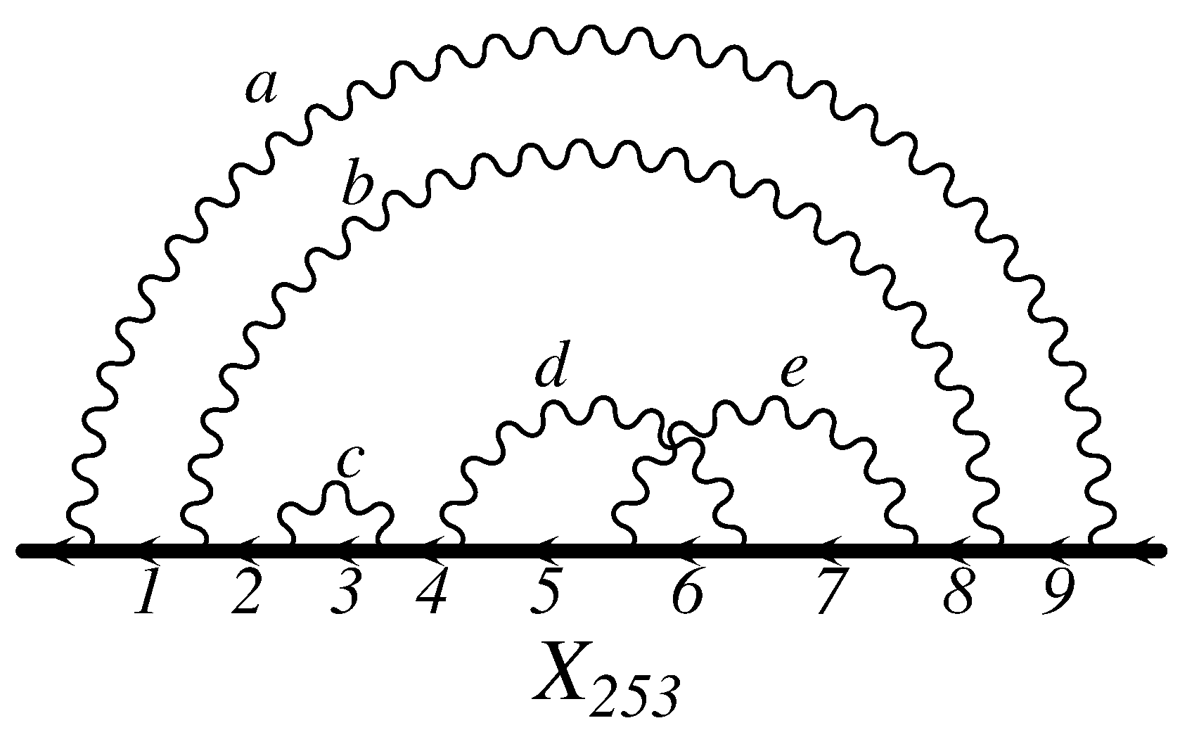
To extend the $\mathbb{K}$-operation procedure for the UV renormalization to a higher order diagram, we need to handle multiple divergences occurring from many subdiagrams contained in it. Let us first list all divergent subdiagrams in a given self-energy diagram. For instance, the tenth-order self-energy diagram $X_{253}$ shown in Figure 7 has five UV divergent subdiagrams: three subdiagrams of a self-energy type, ${\mathcal{S}}_{3c},{\mathcal{S}}_{567de}$, and ${\mathcal{S}}_{2345678bcde}$, and two subdiagrams of a vertex type, ${\mathcal{S}}_{56d}$ and ${\mathcal{S}}_{67e}$. The $\mathbb{K}$-operation renormalized amplitude of ${\Delta }^{\prime }{M}_{X253}$ is formally given by

$${\Delta }^{\prime }{M}_{X253}=(1-{\mathbb{K}}_3)(1-{\mathbb{K}}_{28})(1-{\mathbb{K}}_{56})(1-{\mathbb{K}}_{57})(1-{\mathbb{K}}_{67})M_{X253},$$

(81)

where the electron line numbers of the $\mathbb{K}$-operation are shown as its subscripts to compactify the notation. To construct the UV subtraction terms, the product (81) must be expanded, and the order of multiple $\mathbb{K}$-operations must be changed according to the diagrammatic relations of subdiagrams.

The relation of subdiagrams ${\mathcal{S}}_{\alpha }$ and ${\mathcal{S}}_{\beta }$ can be classified into three cases:

• disjoint: ${\mathcal{S}}_{\alpha }\cap {\mathcal{S}}_{\beta }=\varphi$
  ${\mathcal{S}}_{\alpha }$ and ${\mathcal{S}}_{\beta }$ do not share an electron propagator.
  The operation ${\mathbb{K}}_{\alpha }{\mathbb{K}}_{\beta }$ exists, and ${\mathbb{K}}_{\alpha }$ and ${\mathbb{K}}_{\beta }$ are commutable.
• inclusion: ${\mathcal{S}}_{\alpha }\subset {\mathcal{S}}_{\beta }$
  All electron propagators of ${\mathcal{S}}_{\alpha }$ are also components of ${\mathcal{S}}_{\beta }$.
  The operation ${\mathbb{K}}_{\alpha }{\mathbb{K}}_{\beta }$ exists, and ${\mathbb{K}}_{\alpha }$ and ${\mathbb{K}}_{\beta }$ are not commutable. ${\mathbb{K}}_{\beta }$ must be applied first, and then, ${\mathbb{K}}_{\alpha }$.
• overlapping: ${\mathcal{S}}_{\alpha }\cap {\mathcal{S}}_{\beta }\ne \varphi ,{\mathcal{S}}_{\alpha }\not\subset {\mathcal{S}}_{\beta },{\mathcal{S}}_{\alpha }\not\supset {\mathcal{S}}_{\beta }$
  ${\mathcal{S}}_{\alpha }$ and ${\mathcal{S}}_{\beta }$ partially share the same electron propagators.
  The operations ${\mathbb{K}}_{\alpha }{\mathbb{K}}_{\beta }$ and ${\mathbb{K}}_{\beta }{\mathbb{K}}_{\alpha }$ are null.

Expanding the product (81), we find that 23 UV subtraction terms are needed to make $M_{X253}$ free from UV divergence [59]:

$$\begin{array}{c}{\Delta }^{\prime }{M}_{X253}=[1-{\mathbb{K}}_{56}-{\mathbb{K}}_3-{\mathbb{K}}_{57}-{\mathbb{K}}_{28}-{\mathbb{K}}_{67}+{\mathbb{K}}_3{\mathbb{K}}_{28}+{\mathbb{K}}_{56}{\mathbb{K}}_{28}+{\mathbb{K}}_{67}{\mathbb{K}}_{28}+{\mathbb{K}}_{57}{\mathbb{K}}_{28}+{\mathbb{K}}_3{\mathbb{K}}_{57}\hfill \\ +{\mathbb{K}}_3{\mathbb{K}}_{56}+{\mathbb{K}}_3{\mathbb{K}}_{67}+{\mathbb{K}}_{56}{\mathbb{K}}_{57}+{\mathbb{K}}_{67}{\mathbb{K}}_{57}-{\mathbb{K}}_3{\mathbb{K}}_{67}{\mathbb{K}}_{28}-{\mathbb{K}}_3{\mathbb{K}}_{67}{\mathbb{K}}_{57}-{\mathbb{K}}_3{\mathbb{K}}_{56}{\mathbb{K}}_{28}-{\mathbb{K}}_3{\mathbb{K}}_{56}{\mathbb{K}}_{57}\\ \hfill -{\mathbb{K}}_3{\mathbb{K}}_{57}{\mathbb{K}}_{28}-{\mathbb{K}}_{56}{\mathbb{K}}_{57}{\mathbb{K}}_{28}-{\mathbb{K}}_{67}{\mathbb{K}}_{57}{\mathbb{K}}_{28}+{\mathbb{K}}_3{\mathbb{K}}_{56}{\mathbb{K}}_{57}{\mathbb{K}}_{28}+{\mathbb{K}}_3{\mathbb{K}}_{67}{\mathbb{K}}_{57}{\mathbb{K}}_{28}]M_{X253}.\end{array}$$

(82)

Note that this is a simple realization of Zimmermann’s forest formula [59].

For instance, we can write down the fourth-order amplitudes free from UV divergences:

$$\begin{array}{cc}\hfill {\Delta }^{\prime }{M}_{4a}& =(1-{\mathbb{K}}_{12}-{\mathbb{K}}_{23})M_{4a}=M_{4a}-2L_2^{\mathrm{UV}}{M}_2,\hfill \end{array}$$

(83)

$$\begin{array}{cc}\hfill {\Delta }^{\prime }{M}_{4b}& =(1-{\mathbb{K}}_2)M_{4b}=M_{4b}-\delta m_2^{\mathrm{UV}}{M}_{2^{*}}-B_2^{\mathrm{UV}}{M}_2.\hfill \end{array}$$

(84)

The term corresponding to ${\mathbb{K}}_{12}{\mathbb{K}}_{23}$ is not present, because the relationship between ${\mathcal{S}}_{12a}$ and ${\mathcal{S}}_{23b}$ of $M_{4a}$ is overlapping. The $\mathbb{K}$-operation renormalized amplitude ${\Delta }^{\prime }{M}_{4a}$ is finite. Since the $\mathbb{K}$-operation acts on the integrand, not on the integral, pointwise UV subtraction is realized in the Feynman parameter space. Thus, ${\Delta }^{\prime }{M}_{4a}$ is ready to go to numerical evaluation. We call it the finite amplitude and denote it as $\Delta M_{4a}$ without a prime. The amplitude ${\Delta }^{\prime }{M}_{4b}$ is also free from UV divergence. However, it still suffers from IR divergence. We need to remove it using a pointwise subtraction method.

4.7. IR Divergence

There are two kinds of origins of IR divergence arising in the unrenormalized magnetic moment amplitude $M_{\mathcal{G}}^{\left(2n\right)}$. Both are related to a self-energy subdiagram, but it is not the direct source of IR divergence. Suppose a self-energy-like diagram $\mathcal{G}$ has a self-energy subdiagram $\mathcal{S}$. When the adjacent electron propagators of $\mathcal{S}$ become almost on-the-mass-shell, the residual diagram $\mathcal{G}/\mathcal{S}$ yields IR divergence. Because we use the Ward–Takahashi sum for the magnetic moment amplitude, the self-energy subdiagram $\mathcal{S}$ may have two properties, either the self-mass $\delta m_{\mathcal{S}}$ or the magnetic moment $M_{\mathcal{S}}$ [11].

When the subdiagram $\mathcal{S}$ behaves as a self-mass $\delta m_{\mathcal{S}}$, the residual diagram $\mathcal{G}/\mathcal{S}$ is a magnetic moment amplitude with an insertion of a two-point vertex $M_{{(\mathcal{G}/\mathcal{S})}^{*}}$. This additional vertex increases the number of electron propagators and makes the IR behavior of the amplitude worse than the case without the insertion $M_{\mathcal{G}/\mathcal{S}}$.

To avoid the IR divergence of this kind, we need to complete the mass renormalization with the on-shell condition. The UV divergent part of $\delta m_{\mathcal{S}}$ has been already subtracted by the ${\mathbb{K}}_{\mathcal{S}}$-operation. To subtract the remaining part of the self-mass contribution, we introduce a new procedure, the residual mass renormalization $\mathbb{R}$ such that

$${\mathbb{R}}_{\mathcal{S}}{M}_{\mathcal{G}}=\delta m_{\mathcal{S}}^{\mathrm{R}}\times M_{{(\mathcal{G}/\mathcal{S})}^{*}},$$

(85)

where

$${\delta m}_{\mathcal{S}}^{\mathrm{R}}={\delta m}_{\mathcal{S}}-{\delta m}_{\mathcal{S}}^{\mathrm{UV}}-\left(\mathrm{UV}\mathrm{subdivergences}\right).$$

(86)

When the subdiagram $\mathcal{S}$ yields the magnetic moment $M_{\mathcal{S}}$, the IR behavior of the residual diagram $\mathcal{G}/\mathcal{S}$ is similar to that of the vertex renormalization constant $L_{\mathcal{G}/\mathcal{S}}$ that is obtained by replacing $\mathcal{S}$ by an electron-photon vertex. Thus, we introduce one more procedure, the $\mathbb{I}$-subtraction, such that

$${\mathbb{I}}_{\mathcal{S}}{M}_{\mathcal{G}}=L_{\mathcal{G}/\mathcal{S}}^{\mathrm{R}}\times M_S,$$

(87)

where

$$L_{\mathcal{G}/\mathcal{S}}^{\mathrm{R}}=L_{\mathcal{G}/\mathcal{S}}-L_{\mathcal{G}/\mathcal{S}}^{\mathrm{UV}}-\left(\mathrm{UV}\mathrm{subdivergences}\right).$$

(88)

The UV divergences arising in the IR subtraction terms (85) and (87) are removed by using the $\mathbb{K}$-operation renormalization. Decoupled products of (85) and (87) are merged into the same Feynman parametric space of $M_{\mathcal{G}}$ by applying the technique to derive (72) or (79) inversely.

All IR divergences of the magnetic moment amplitude $M_{\mathcal{G}}^{\left(2n\right)}$ can be removed by the above two IR subtractions. For nested IR divergences appearing in a higher order diagram, we prepare the annotated forest formula and apply the $\mathbb{R}$- and/or $\mathbb{I}$-subtractions as needed. There are two types of relations between two self-energy subdiagrams ${\mathcal{S}}_{\alpha }$ and ${\mathcal{S}}_{\beta }$. Namely,

• disjoint: ${\mathcal{S}}_{\alpha }\cap {\mathcal{S}}_{\beta }=\varphi$

  (a)

  One of the $\mathcal{S}$’s is a magnetic moment, and another is a self-mass: ${\mathbb{I}}_{{\mathcal{S}}_{\beta }}{\mathbb{R}}_{{\mathcal{S}}_{\alpha }}+{\mathbb{I}}_{{\mathcal{S}}_{\alpha }}{\mathbb{R}}_{{\mathcal{S}}_{\beta }}$.

  (b)

  Both are self-masses: ${\mathbb{R}}_{{\mathcal{S}}_{\alpha }}{\mathbb{R}}_{{\mathcal{S}}_{\beta }}$.

  (c)

  Two $\mathcal{S}$’s cannot simultaneously become magnetic moments: No double $\mathbb{I}$-subtractions.

• inclusion: ${\mathcal{S}}_{\alpha }\subset {\mathcal{S}}_{\beta }$

  (a)

  If ${\mathcal{S}}_{\alpha }$ is a magnetic moment, ${\mathcal{S}}_{\beta }$ cannot be a self-mass: ${\mathbb{I}}_{{\mathcal{S}}_{\alpha }}{\mathbb{I}}_{{\mathcal{S}}_{\beta }}$.

  (b)

  Both S’s are self-masses: ${\mathbb{R}}_{{\mathcal{S}}_{\beta }/{\mathcal{S}}_{\alpha }}{\mathbb{R}}_{\alpha }$.

  (c)

  ${\mathcal{S}}_{\alpha }$ is a self-mass, and ${\mathcal{S}}_{\beta }$ is a magnetic moment: ${\mathbb{R}}_{\alpha }{\mathbb{I}}_{{\mathcal{S}}_{\beta }}$.

As an example, let us construct the IR subtraction terms for the tenth-order diagram $X_{253}$ shown in Figure 7. There are three self-energy subdiagrams ${\mathcal{S}}_{3c}$, ${\mathcal{S}}_{567de}$, and ${\mathcal{S}}_{2345678bcde}$. Because $\delta m_2^{\mathrm{R}}=0$ in our definition, the residual mass renormalization for ${\mathcal{S}}_{3c}$ is not needed. We find

$$\begin{array}{c}\Delta M_{X253}=[1-{\mathbb{R}}_{28}-{\mathbb{R}}_{57}-{\mathbb{I}}_{12456789}-{\mathbb{I}}_{123489}-{\mathbb{I}}_{19}+{\mathbb{I}}_{19}{\mathbb{I}}_{245678}\hfill \\ \hfill +{\mathbb{I}}_{19}{\mathbb{I}}_{2348}+{\mathbb{R}}_{28}{\mathbb{R}}_{57}+{\mathbb{I}}_{19}{\mathbb{R}}_{57}+{\mathbb{I}}_{12489}{\mathbb{R}}_{57}-{\mathbb{I}}_{19}{\mathbb{I}}_{248}{\mathbb{R}}_{57}]{\Delta }^{\prime }{M}_{X253}.\end{array}$$

(89)

The IR-subtraction terms for the unrenormalized amplitude $M_{X253}$ are produced first by using the multiple $\mathbb{R}$ and/or $\mathbb{I}$-subtractions. Then, the UV divergences of these IR-subtraction terms are removed by using the $\mathbb{K}$-operation described in Section 4.5 and Section 4.6. The latter part of the construction of the IR-subtraction terms is symbolically written as the application of $\mathbb{R}$- and/or $\mathbb{I}$-operations to the UV-free amplitude ${\Delta }^{\prime }{M}_{X253}$.

In a similar fashion, we apply the $\mathbb{R}$- and $\mathbb{I}$-subtractions to $M_{4b}$, and the finite amplitude $\Delta M_{4b}$ is obtained as

$$\Delta M_{4b}=(1-{\mathbb{R}}_2-{\mathbb{I}}_{13}){\Delta }^{\prime }{M}_{4b}=M_{4b}-\delta m_2^{\mathrm{UV}}{M}_{2^{*}}-B_2^{\mathrm{UV}}{M}_2-\delta m_2^{\mathrm{R}}{M}_{2^{*}}-L_2^{\mathrm{R}}{M}_2.$$

(90)

This is ready to go to numerical calculation. In fact, because of our definition of the $\mathbb{K}$-operation, we have $\delta m_2=\delta m_2^{\mathrm{UV}}$ and $\delta m_2^{\mathrm{R}}=0$. This simplifies the calculation of the physical contribution of $a_e$, especially for the higher order terms.

4.8. Residual Renormalization

The UV renormalization we have employed is not the standard on-shell renormalization. In addition, the $\mathbb{K}$-operation renormalization, which is a simple power counting rule of contractions and Feynman parameters, violates the Ward–Takahashi identity between the renormalization constants:

$$L_2^{\mathrm{UV}}+B_2^{\mathrm{UV}}\ne 0.$$

(91)

We also artificially added IR subtraction terms in order to make the amplitude numerically calculable on a computer. The residual and finite renormalization procedure is to be introduced to obtain the physical contribution to $a_e$ from the numerically-calculated finite amplitudes. During this process, the violation of the Ward–Takahashi identity of the renormalization constants is fixed. Then, the gauge invariance of the physical contribution to $a_e$ is guaranteed. It is also used to check the IR cancellation in the physical contribution to $a_e$ as stated by the Kinoshita–Lee–Nauenberg theorem [57,60].

Let us explicitly work out the fourth-order case. The standard renormalization procedure for the diagrams $M_{4a}$ and $M_{4b}$ can be expressed by using the finite amplitudes given in (83) and (90). We find

$$\begin{array}{c}{a}_{4a}\equiv M_{4a}-2L_2{M}_2=\Delta M_{4a}-2L_2^{\mathrm{R}}{M}_2,\hfill \end{array}$$

(92)

$$\begin{array}{c}{a}_{4b}\equiv M_{4b}-\delta m_2{M}_{2^{*}}-B_2{M}_2=\Delta M_{4b}-B_2^{\mathrm{R}}{M}_2+L_2^{\mathrm{R}}{M}_2.\hfill \end{array}$$

(93)

Thus, the physical contribution from the gauge-invariant set of the fourth-order becomes

$$a_4\equiv a_{4a}+a_{4b}=\Delta M_{4a}+\Delta M_{4b}-\Delta L{B}_2{M}_2,$$

(94)

where

$$\Delta L{B}_2\equiv L_2^{\mathrm{R}}+B_2^{\mathrm{R}}$$

(95)

is guaranteed to be finite because of the Ward–Takahashi identity. Thus, all three terms in the right-hand-side of (94) are finite, and the physical contribution $a_4$ is free from IR divergences. After numerical integration, the finite quantities in (94) are found:

$$\begin{array}{cccc}\hfill \Delta M_{4a}& =0.218347\left(32\right){\left(\frac{\alpha }{\pi }\right)}^2,\hfill & \hfill \Delta M_{4b}& =-0.187478\left(35\right){\left(\frac{\alpha }{\pi }\right)}^2,\hfill \\ \hfill M_2& =0.5\left(\frac{\alpha }{\pi }\right),\hfill & \hfill \Delta L{B}_2& =0.75\left(\frac{\alpha }{\pi }\right),\hfill \end{array}$$

(96)

and we obtain

$$a_4=-0.344131\left(48\right){\left(\frac{\alpha }{\pi }\right)}^2,$$

(97)

which is in agreement with the analytic result $-0.344166\cdots {(\alpha /\pi )}^2$.

As you can see from the derivation of it, an explicit recipe of the $\mathbb{K}$-operation is not essential to derive the finite formula (94). The on-shell mass renormalization is mandatory to make an integral free from IR divergence and available for numerical calculation. However, the separation of UV and residual terms of the vertex and wave-function renormalization constants can be arbitrary and is not necessarily the $\mathbb{K}$-operation. For instance, S. Volkov used the separation such that the Ward–Takahashi identity holds [15,61]:

$$\sum _{i\in S}{L}_{S_{\left(i\right)}}^{\mathrm{UV}}+B_S^{\mathrm{UV}}=0,$$

(98)

where $\left(i\right)$ indicates that the electron-photon vertex is inserted in the electron propagator i of the self-energy diagram S and the sum is taken over all electron propagators of S. Thus, no residual renormalization is required. In [15,61], this method is applied to numerical calculation of the eighth-order vertex diagrams without a fermion loop. The result is consistent with the previous numerical calculation formulated by using the $\mathbb{K}$-operation [39] and also the analytic calculation [26].

5. Higher Order Calculation

For the higher order diagrams without a fermion loop, we have applied the same process described in Section 4 to calculate the contributions to $a_e$. Because of the complexity and length of finite integrals of the higher orders, especially of the tenth-order, we automated many of the procedures described in Section 4 [10,11].

The automatic code generator of the integrand of a given self-energy-like diagram without a fermion loop is called gencodeN. It is applicable to any order self-energy-like diagrams up to tenth-order and is extendable to even higher orders. From one-line information representing a self-energy diagram $\mathcal{G}$ of the $2n\mathrm{th}$-order, it generates the integrand of the finite amplitude $\Delta M_{\mathcal{G}}$ as a set of FORTRAN programs. It can be numerically evaluated with multi-dimensional integration algorithm, such as VEGAS [62]. The workflow of gencodeN is the following:

• The one-line input of self-energy-like diagrams $\mathcal{G}$ is given. It is a sequence of the names of photons attached to the electron propagators from left to right. For example, the tenth-order diagram $X_{253}$ of Figure 7 is represented by “$abccdedeba$.”
• The integrand of the unrenormalized magnetic amplitude $M_{\mathcal{G}}$ is determined. More precisely, the numerator functions $N_i,E_i,Z_i,$, and $C_i$ are determined in terms of the building blocks and the scalar currents.
• The building blocks $B_{ij}$’s and U are determined in terms of the Feynman parameters from the topology of $\mathcal{G}$.
• The forest formula for UV divergences of $\mathcal{G}$ is constructed. UV subtraction terms are then generated in terms of the building blocks.
• The UV limit of the building blocks $B_{ij}$ and U is taken for each UV subtraction term.
• The annotated forest formula for IR divergences of $\mathcal{G}$ is constructed. IR subtraction terms are then generated. The building blocks $B_{ij}$’s and U of the UV subtraction terms that show the same decoupling of the subdiagrams are borrowed and used.
• The integrand of the finite amplitude $\Delta M_{\mathcal{G}}$ is constructed combining together all of the above.

The 6354 vertex diagrams of Set V of the tenth-order as shown in Figure 5 can be reduced to 389 self-energy-like subdiagrams. The 389 integrands, each consisting of about 100,000 lines of FORTRAN code, are generated by gencodeN running on a personal computer. While numerical integration of the 389 finite amplitudes of $\Delta M_{\mathcal{G}}$ are being carried out on supercomputers, the residual renormalization formula of the $2n\mathrm{th}$-order is derived from the symbolic manipulation like (94). Neither numerical calculation, nor difficult algebraic calculation are needed at this stage. For the tenth-order case, we obtain

$$\begin{array}{cc}\hfill A_1^{\left(10\right)}\left[\mathrm{Set}\mathrm{V}\right]=& \Delta M_{10}\hfill \\ \hfill +& \Delta M_8(-7\Delta L{B}_2)\hfill \\ \hfill +& \Delta M_6\{-5\Delta L{B}_4+20{(\Delta L{B}_2)}^2\}\hfill \\ \hfill +& \Delta M_4\{-3\Delta L{B}_6+24\Delta L{B}_4\Delta L{B}_2-28{(\Delta L{B}_2)}^3\}\hfill \\ \hfill +& \Delta M_4(2\Delta \delta m_4\Delta L_{2^{*}})\hfill \\ \hfill +& M_2\{-\Delta L{B}_8+8\Delta L{B}_6\Delta L{B}_2-28\Delta L{B}_4{(\Delta L{B}_2)}^2\hfill \\ & +4{(\Delta L{B}_4)}^2+14{(\Delta L{B}_2)}^4\}\hfill \\ \hfill +& M_2\Delta \delta m_6(2\Delta L_{2^{*}})\hfill \\ \hfill +& M_2\Delta \delta m_4(-16\Delta L{B}_2\Delta L_{2^{*}}-2\Delta \delta m_{2^{*}}\Delta L_{2^{*}}+\Delta L_{4^{*}}).\hfill \end{array}$$

(99)

The finite integrals $\Delta M_{2n}$, $\Delta L{B}_{2n}$, $\Delta \delta m_{2n}$ are obtained from the magnetic moment amplitudes, the sum of vertex and wave-function renormalization constants, and the mass renormalization constants, respectively, of the $2n\mathrm{th}$-order diagrams without a fermion loop. An asterisk (∗) indicates that the quantity can be derived from diagrams having a two-point vertex insertion. For instance, $\Delta L_{4^{*}}$ is the sum of finite parts of 24 diagrams, which are fourth-order vertices with a two-point vertex in one of four electron propagators. Some quantities appearing in (99) are identical with those used in the lower order calculations such as the sixth- and eighth-order contributions. Agreement between the analytic results and the numerical results obtained by using these quantities is indirect, but strong evidence that they are correct.

Newly-evaluated ones specifically for the tenth-order are $\Delta L{B}_8$, $\Delta \delta m_6$, and $\Delta L_{4^{*}}$. The sixth- and fourth-order quantities are easily calculated. For $\Delta L{B}_8$, we prepared another code generator gencodeLBN similar to gencodeN by changing projection operators. The 47 integrals for $\Delta L{B}_8$ were then numerically evaluated. The numerical values of all finite integrals in (99) are listed in

Table 3. Residual renormalization constants used to calculate $A_1^{\left(10\right)}\left[\mathrm{Set}\mathrm{V}\right]$. The $\Delta M_{2n}$, $\Delta L{B}_{2n}$, and $\Delta d{m}_{2n}$ are the sum of the finite magnetic moment amplitudes, the sum of the finite parts of vertex and wave-function renormalization constants, and the sum of the finite parts of the mass-renormalization constants, respectively, all derived from the $2n\mathrm{th}$-order diagrams without a fermion loop of the QED perturbation theory. They are given in units of ${(\alpha /\pi )}^{2n}$. $\Delta M_{10}$ is newly calculated for this paper. $\Delta M_8$ is derived from the near-exact result Equation (5) of [26].

Integral	Value (Error)
$\Delta M_{10}$	2.412 (159)
$\Delta M_8$	1.738 467 (20)
$\Delta M_6$	0.425 8135 (30)
$\Delta M_4$	0.030 833 612⋯
$M_2$	0.5
$\Delta L{B}_8$	2.0504 (86)
$\Delta L{B}_6$	0.100 801 (43)
$\Delta L{B}_4$	0.027 9171 (61)
$\Delta L{B}_2$	0.75
$\Delta L_{4^{*}}$	−0.459 051 (62)
$\Delta L_{2^{*}}$	−0.75
$\Delta \delta m_6$	−2.340 815 (55)
$\Delta \delta m_4$	1.906 3609 (90)
$\Delta \delta m_{2^{*}}$	−0.75

. Many of them are borrowed from [40]. The tenth-order finite magnetic moment amplitude is updated in this work as

$$\Delta M_{10}\equiv \sum _{\mathcal{G}=X001}^{X389}\Delta M_{\mathcal{G}}=2.412\left(159\right),$$

(100)

in units of ${(\alpha /\pi )}^5$. The factor two of each time-reversal-symmetric diagram is included in the numerical value of $\Delta M_{\mathcal{G}}$. The improvement of the numerical value of $\Delta M_{10}$ leads to a new tenth-order contribution $A_1^{\left(10\right)}$ of (8).

6. Conclusions

An overview of the current status of the standard model prediction of the electron anomalous magnetic moment $a_e$ is given. The fine-structure constant determined from measurements in atomic physics is the dominant source of the uncertainty of $a_e$. Both numerical and analytic works on the QED contribution have succeeded in reducing its uncertainty. By now, the hadronic contribution is the second largest source of uncertainty in the standard model prediction of $a_e$. The method of numerical computation of the higher order QED contributions to $a_e$, especially those from diagrams without a fermion loop, is described in some detail.

References

- Kusch, P.; Foley, H.M. Precision Measurement of the Ratio of the Atomic ‘g Values’ in the 2P3/2 and 2P1/2 States of Gallium. Phys. Rev. 1947, 72, 1256–1257. [Google Scholar] [CrossRef]
- Lamb, W.E., Jr.; Retherford, R.C. Fine Structure of the Hydrogen Atom by a Microwave Method. Phys. Rev. 1947, 72, 241. [Google Scholar] [CrossRef]
- Heisenberg, W.; Pauli, W. On Quantum Field Theory. Z. Phys. 1929, 56, 1–61. (In German) [Google Scholar] [CrossRef]
- Heisenberg, W.; Pauli, W. On Quantum Field Theory. 2. Z. Phys. 1930, 59, 168–190. (In German) [Google Scholar] [CrossRef]
- Schwinger, J.S. On Quantum electrodynamics and the magnetic moment of the electron. Phys. Rev. 1948, 73, 416–417. [Google Scholar] [CrossRef]
- Aldins, J.; Kinoshita, T.; Brodsky, S.J.; Dufner, A.J. Photon-Photon Scattering Contribution to the Sixth Order Magnetic Moments Of The Muon And Electron. Phys. Rev. D 1970, 1, 2378. [Google Scholar] [CrossRef]
- Cvitanović, P.; Kinoshita, T. Feynman-Dyson rules in parametric space. Phys. Rev. D 1974, 10, 3978. [Google Scholar] [CrossRef]
- Cvitanović, P.; Kinoshita, T. New Approach to the Separation of Ultraviolet and Infrared Divergences of Feynman—Parametric Integrals. Phys. Rev. D 1974, 10, 3991. [Google Scholar] [CrossRef]
- Kinoshita, T. Theory of the Anomalous Magnetic Moment of the Electron-Numerical Approach. In Quantum Electrodynamics; Kinoshita, T., Ed.; World Scientific: Singapore, 1990; pp. 218–321. [Google Scholar]
- Aoyama, T.; Hayakawa, M.; Kinoshita, T.; Nio, M. Automated calculation scheme for αn contributions of QED to lepton g-2: Generating renormalized amplitudes for diagrams without lepton loops. Nucl. Phys. B 2006, 740, 138–180. [Google Scholar] [CrossRef]
- Aoyama, T.; Hayakawa, M.; Kinoshita, T.; Nio, M. Automated Calculation Scheme for αn Contributions of QED to Lepton g-2: New Treatment of Infrared Divergence for Diagrams without Lepton Loops. Nucl. Phys. B 2008, 796, 184–210. [Google Scholar] [CrossRef]
- Aoyama, T.; Hayakawa, M.; Kinoshita, T.; Nio, M. Quantum Electrodynamics Calculation of Lepton Anomalous Magnetic Moments: Numerical Approach to the Perturbation Theory of QED. Prog. Theor. Exp. Phys. 2012, 2012, 01A107. [Google Scholar] [CrossRef]
- Levine, M.J.; Wright, J. Anomalous magnetic moment of the electron. Phys. Rev. D 1973, 8, 3171–3179. [Google Scholar] [CrossRef]
- Carroll, R. Mass Operator Calculation of the electron G-Factor. Phys. Rev. D 1975, 12, 2344. [Google Scholar] [CrossRef]
- Volkov, S. New method of computing the contributions of graphs without lepton loops to the electron anomalous magnetic moment in QED. Phys. Rev. D 2017, 96, 096018. [Google Scholar] [CrossRef]
- Fujikawa, K.; Lee, B.; Sanda, A. Generalized Renormalizable Gauge Formulation of Spontaneously Broken Gauge Theories. Phys. Rev. D 1972, 6, 2923–2943. [Google Scholar] [CrossRef]
- Czarnecki, A.; Krause, B.; Marciano, W.J. Electroweak corrections to the muon anomalous magnetic moment. Phys. Rev. Lett. 1996, 76, 3267–3270. [Google Scholar] [CrossRef] [PubMed]
- Knecht, M.; Peris, S.; Perrottet, M.; De Rafael, E. Electroweak hadronic contributions to g(mu)-2. J. High Energy Phys. 2002, 11, 003. [Google Scholar] [CrossRef]
- Czarnecki, A.; Marciano, W.J.; Vainshtein, A. Refinements in electroweak contributions to the muon anomalous magnetic moment. Phys. Rev. D 2003, 67, 073006. [Google Scholar] [CrossRef]
- Nomura, D.; Teubner, T. Hadronic contributions to the anomalous magnetic moment of the electron and the hyperfine splitting of muonium. Nucl. Phys. B 2013, 867, 236–243. [Google Scholar] [CrossRef]
- Kurz, A.; Liu, T.; Marquard, P.; Steinhauser, M. Hadronic contribution to the muon anomalous magnetic moment to next-to-next-to-leading order. Phys. Lett. B 2014, 734, 144–147. [Google Scholar] [CrossRef]
- Jegerlehner, F. Variations on Photon Vacuum Polarization. arXiv, 2017; arXiv:1711.06089. [Google Scholar]
- Petermann, A. Fourth order magnetic moment of the electron. Helv. Phys. Acta 1957, 30, 407–408. [Google Scholar] [CrossRef]
- Sommerfield, C.M. The magnetic moment of the electron. Ann. Phys. 1958, 5, 26–57. [Google Scholar] [CrossRef]
- Laporta, S.; Remiddi, E. The analytical value of the electron (g-2) at order α 3 in QED. Phys. Lett. B 1996, 379, 283–291. [Google Scholar] [CrossRef]
- Laporta, S. High-precision calculation of the 4-loop contribution to the electron g-2 in QED. Phys. Lett. B 2017, 772, 232–238. [Google Scholar] [CrossRef]
- Elend, H.H. On the anomalous magnetic moment of the muon. Phys. Lett. 1966, 20, 682–684. [Google Scholar] [CrossRef]
- Samuel, M.A.; Li, G.W. Improved analytic theory of the muon anomalous magnetic moment. Phys. Rev. D 1991, 44, 3935–3942. [Google Scholar] [CrossRef]
- Li, G.; Mendel, R.; Samuel, M.A. Precise mass ratio dependence of fourth order lepton anomalous magnetic moments: The Effect of a new measurement of m(tau). Phys. Rev. D 1993, 47, 1723–1725. [Google Scholar] [CrossRef]
- Laporta, S.; Remiddi, E. The Analytical value of the electron light-light graphs contribution to the muon (g-2) in QED. Phys. Lett. B 1993, 301, 440–446. [Google Scholar] [CrossRef]
- Laporta, S. The Analytical contribution of the sixth order graphs with vacuum polarization insertions to the muon (g-2) in QED. Nuovo Cimento A 1993, 106, 675–683. [Google Scholar] [CrossRef]
- Kurz, A.; Liu, T.; Marquard, P.; Steinhauser, M. Anomalous magnetic moment with heavy virtual leptons. Nucl. Phys. B 2014, 879, 1–18. [Google Scholar] [CrossRef]
- Kinoshita, T. New value of the alpha3 electron anomalous magnetic moment. Phys. Rev. Lett. 1995, 75, 4728–4731. [Google Scholar] [CrossRef] [PubMed]
- Melnikov, K.; van Ritbergen, T. The Three loop slope of the Dirac form-factor and the S Lamb shift in hydrogen. Phys. Rev. Lett. 2000, 84, 1673–1676. [Google Scholar] [CrossRef] [PubMed]
- Aoyama, T.; Hayakawa, M.; Kinoshita, T.; Nio, M. Tenth-Order QED Contribution to the Electron g-2 and an Improved Value of the Fine Structure Constant. Phys. Rev. Lett. 2012, 109, 111807. [Google Scholar] [CrossRef] [PubMed]
- Laporta, S. High precision calculation of multiloop Feynman integrals by difference equations. Int. J. Mod. Phys. A 2000, 15, 5087–5159. [Google Scholar] [CrossRef]
- Ferguson, H.R.P.; Bailey, D.H. A Polynomial Time, Numerically Stable Integer Relation Algorithm; Technical Report, RNR-91-032; 1992. [Google Scholar]
- Bailey, D.H.; Broadhurst, D.J. Parallel Integer Relation Detection: Techniques and Applications. Math. Comput. 2001, 70, 1719–1736. [Google Scholar] [CrossRef]
- Aoyama, T.; Hayakawa, M.; Kinoshita, T.; Nio, M. Tenth-Order Electron Anomalous Magnetic Moment—Contribution of Diagrams without Closed Lepton Loops. Phys. Rev. D 2015, 91, 033006. [Google Scholar] [CrossRef]
- Aoyama, T.; Kinoshita, T.; Nio, M. Revised and Improved Value of the QED Tenth-Order Electron Anomalous Magnetic Moment. Phys. Rev. D 2018, 97, 036001. [Google Scholar] [CrossRef]
- Mohr, P.J.; Newell, D.B.; Taylor, B.N. CODATA Recommended Values of the Fundamental Physical Constants: 2014. Rev. Mod. Phys. 2016, 88, 035009. [Google Scholar] [CrossRef]
- Tanabashi, M.; Hagiwara, K.; Hikasa, K.; Nakamura, K.; Sumino, Y.; Takahashi, F.; Tanaka, J.; Agashe, K.; Aielli, G.; Amsler, C.; et al. Review of Particle Physics. Phys. Rev. D 2018, 98, 030001. [Google Scholar] [CrossRef]
- Passera, M. Precise mass-dependent QED contributions to leptonic g-2 at order α2 and α3. Phys. Rev. D 2007, 75, 013002. [Google Scholar] [CrossRef]
- Kasevich, M.; Chu, S. Atomic interferometry using stimulated Raman transitions. Phys. Rev. Lett. 1991, 67, 181–184. [Google Scholar] [CrossRef] [PubMed]
- Cladé, P.; De Mirandes, E.; Cadoret, M.; Guellati-Khélifa, S.; Schwob, C.; Nez, F.; Julien, L.; Biraben, F. Determination of the Fine Structure Constant Based on Bloch Oscillations of Ultracold Atoms in a Vertical Optical Lattice. Phys. Rev. Lett. 2006, 96, 033001. [Google Scholar] [CrossRef] [PubMed]
- Beyer, A.; Maisenbacher, L.; Matveev, A.; Pohl, R.; Khabarova, K.; Grinin, A.; Lamour, T.; Yost, D.C.; Hänsch, T.W.; Kolachevsky, N.; et al. The Rydberg constant and proton size from atomic hydrogen. Science 2017, 358, 79–85. [Google Scholar] [CrossRef] [PubMed]
- Fleurbaey, H.; Galtier, S.; Thomas, S.; Bonnaud, M.; Julien, L.; Biraben, F.M.C.; Nez, F.M.C.; Abgrall, M.; Guéna, J. New Measurement of the 1S − 3S Transition Frequency of Hydrogen: Contribution to the Proton Charge Radius Puzzle. Phys. Rev. Lett. 2018, 120, 183001. [Google Scholar] [CrossRef] [PubMed]
- Bouchendira, R.; Clade, P.; Guellati-Khelifa, S.; Nez, F.; Biraben, F. New determination of the fine structure constant and test of the quantum electrodynamics. Phys. Rev. Lett. 2011, 106, 080801. [Google Scholar] [CrossRef] [PubMed]
- Parker, R.H.; Yu, C.; Zhong, W.; Estey, B.; Müller, H. Measurement of the fine-structure constant as a test of the Standard Model. Science 2018, 360, 191–195. [Google Scholar] [CrossRef] [PubMed]
- Hanneke, D.; Fogwell, S.; Gabrielse, G. New Measurement of the Electron Magnetic Moment and the Fine Structure Constant. Phys. Rev. Lett. 2008, 100, 120801. [Google Scholar] [CrossRef] [PubMed]
- Adkins, G.S. Feynman Rules Of Coulomb Gauge Qed And The Electron Magnetic Moment. Phys. Rev. D 1987, 36, 1929–1932. [Google Scholar] [CrossRef]
- Cvitanovic, P.; Lautrup, B.; Pearson, R.B. The Number And Weights Of Feynman Diagrams. Phys. Rev. D 1978, 18, 1939. [Google Scholar] [CrossRef]
- Itzykson, C.; Zuber, J.B. Functional Methods. In Quantum Field Theory; McGRAW-HILL: New York, NY, USA, 1980; Chapter 9. [Google Scholar]
- Baikov, P.A.; Broadhurst, D.J. Three loop QED vacuum polarization and the four loop muon anomalous magnetic moment. In Proceedings of the 4th International Workshop on Software Engineering, Artificial Intelligence, and Expert Systems for High-Energy and Nuclear Physics (AIHENP95), Pisa, Italy, 3–8 April 1995; pp. 167–172. [Google Scholar]
- Baikov, P.A.; Maier, A.; Marquard, P. The QED vacuum polarization function at four loops and the anomalous magnetic moment at five loops. Nucl. Phys. B 2013, 877, 647–661. [Google Scholar] [CrossRef]
- Kurz, A.; Liu, T.; Marquard, P.; Smirnov, A.V.; Smirnov, V.A.; Steinhauser, M. Light-by-light-type corrections to the muon anomalous magnetic moment at four-loop order. Phys. Rev. D 2015, 92, 073019. [Google Scholar] [CrossRef]
- Kinoshita, T. Mass singularities of Feynman amplitudes. J. Math. Phys. 1962, 3, 650–677. [Google Scholar] [CrossRef]
- Nakanishi, N. Graph Theory and Feynman Integrals; Gordon and Breach, Science Publishers: New York, NY, USA, 1971. [Google Scholar]
- Zimmermann, W. Convergence of Bogolyubov’s method of renormalization in momentum space. Commun. Math. Phys. 1969, 15, 208–234. [Google Scholar] [CrossRef]
- Lee, T.D.; Nauenberg, M. Degenerate Systems and Mass Singularities. Phys. Rev. 1964, 133, B1549–B1562. [Google Scholar] [CrossRef]
- Volkov, S. Numerical calculation of high-order QED contributions to the electron anomalous magnetic moment. Phys. Rev. D 2018, 98, 076018. [Google Scholar] [CrossRef]
- Lepage, G.P. A New Algorithm for Adaptive Multidimensional Integration. J. Comput. Phys. 1978, 27, 192–203. [Google Scholar] [CrossRef]
Figure 1.
Second-order vertex diagram. There is only one diagram. The straight and wavy lines represent electron and photon propagators, respectively. Reprinted from [12].
Figure 2.
Fourth-order vertex diagrams. There are seven diagrams in total. The time-reversal diagrams of (a,c) are not shown. The solid and wavy lines represent electron and photon propagators, respectively. Reprinted from [12].
Figure 3.
Sixth-order vertex diagrams. There are 72 diagrams in total, and they are divided into five gauge-invariant sets. Typical diagrams from each set are shown as (a–e). There are (a) 3 diagrams, (b) 1 diagram, (c) 12 diagrams, (d) 6 diagrams, and (e) 50 diagrams. The solid and wavy lines represent electron and photon propagators, respectively. Reprinted from [12].
Figure 4.
Eighth-order vertex diagrams. There are 891 diagrams in total, and they are divided into 13 gauge-invariant subsets of five super sets. A typical diagram from each subset is shown as I(a–d), II(a–c), III, IV(a–d), and V. There are I(a) 1 diagram, I(b) 6 diagrams, I(c) 3 diagrams, I(d) 15 diagrams, II(a) 36 diagrams, II(b) 6 diagrams, II(c) 12 diagrams, III 150 diagrams, IV(a) 18 diagrams, IV(b) 60 diagrams, IV(c) 48 diagrams, IV(d) 18 diagrams, and V 518 diagrams. The straight and wavy lines represent electron and photon propagators, respectively. Reprinted from [12].
Figure 5.
Tenth-order vertex diagrams. There are 12,672 diagrams in total, and they are divided into 32 gauge-invariant subsets over six super sets. Typical diagrams of each subsets are shown as I(a–j), II(a–f), III(a–c), IV, V, and VI(a–k). There are Set I 208 diagrams (I(a) 1, I(b) 9, I(c) 9, I(d) 6, I(e) 30, I(f) 3, I(g) 9, I(h) 30, I(i) 105, I(j) 6), Set II 600 diagrams (II(a) 24, II(b) 108, II(c) 36, II(d) 180, II(e) 180, II(f) 72), Set III 1140 diagrams (III(a) 300, III(b) 450, III(c) 390), Set IV 2072 diagrams, Set V 6354 diagrams, Set VI 2298 diagrams (VI(a) 36, VI(b) 54, VI(c) 144, VI(d) 492, VI(e) 48, VI(f) 180, VI(g) 480, VI(h) 630, VI(i) 60, VI(j) 54, VI(k) 120). The straight and wavy lines represent electron and photon propagators, respectively. The external photon vertex is omitted for simplicity and can be attached to one of the electron propagators of the bottom straight line in super sets I–V or the large ellipse in super set VI. Reprinted from [12].
Figure 6.
Fourth-order self-energy-like diagrams, and . The solid and wavy lines represent electron and photon propagators, respectively.
Figure 7.
A tenth-order self-energy-like diagram. This is one of the diagrams V of Figure 5. The solid and wavy lines represent electron and photon propagators, respectively. Reprinted from [39].