Progress in Finding New Energy Levels Using Laser Spectroscopy

Institute of Experimental Physics, Graz University of Technology, Petersgasse 16, A-8010 Graz, Austria
Atoms 2018, 6(4), 54; https://doi.org/10.3390/atoms6040054
Submission received: 23 July 2018
/
Revised: 12 September 2018
/
Accepted: 20 September 2018
/
Published: 25 September 2018
(This article belongs to the Special Issue Current Developments and Applications of Atomic Structure and Radiative Process Investigations)
Abstract
:The necessary tools for determining a fast and, during an experimental run, possible location of a new energy level are presented, using the findings and characterization of a new level of the La atom as an example. Due to the corresponding computer programs, the observations gained during the experiment can be immediately used.
1. Introduction
Despite the usual meaning that the fine structure energy levels of nearly all atoms (and their ions with a low number of removed electrons) have been known for several decades, a closer look shows that this is not true. The commonly used tables (e.g., [1,2,3]) are by far not complete and sometimes even contain levels which are not existing. Thus, in some cases spectral lines, which are used for an analysis of the spectra of stars etc. are not correctly classified. Additionally, for semi-emperical or ab initio theoretical investigations of the electronic structure of atoms, complete and correct lists of energy levels are needed. In addition to the energy values, parity, angular momenta, hyperfine (hf) structure constants, and Lande-factors should also be determined reliably.
For finding energy levels—as done in the past—the emission spectrum of an element has to be investigated. Knowledge of the spectra in a wide range, from UV to infrared, makes the analysis easier, depending on the investigated atomic system. High-resolution spectrographs and photographic recording (on photo plates) enabled to classify most spectral lines of the chemical elements. The most famous collections of energy levels are the tables of C. Moore [1] and the NIST atomic database [2], and for the lanthanides [3]. Thus classical emission spectroscopy is the most important source of energy levels of atoms and their first ions.
The resolution of the spectra could be enhanced using computer-aided Fourier-transform (FT) spectroscopy, resolving even the hf structure splitting of the spectral lines, if this splitting is larger than the apparatus profile. The advantages of FT spectroscopy are:
- -
- wide wavelength range;
- -
- very good resolution; and
- -
- very large dynamical range.
Thus, a classification of spectral lines due to wave number and hf pattern is possible.
With the invention of continuously-tunable lasers, laser spectroscopy put atomic spectroscopy a forward significant step. The advantages of tunable, frequency-stabilized laser light are:
- -
- Doppler-limited resolution or even higher (Doppler-free or Doppler-reduced methods); and
- -
- much more sensitivity due to the high spectral energy density.
However, the recording of the overview spectra is very time consuming and needs methods which are not sensitive to the excited energy levels.
2. Laser-Spectroscopic Experiment
As a source of free atoms, a see-through hollow cathode discharge is used. The discharge starts in a noble gas of less than 1 mbar pressure; in most cases, Ar or Ne. After some minutes a sputtering process sets in, and the discharge is carried more and more by the sputtered metal vapor (comparable to the starting process of a low-pressure sodium lamp). The discharge becomes bright and colored typically for the investigated element (e.g., green for Pr, white for La). Due to the discharge, all energy levels of the investigated element are populated sufficiently to perform laser excitation to higher lying levels. The discharge is cooled with liquid nitrogen to enhance the sputtering process, to make the discharge less noisy, and to reduce the Doppler width of the recorded spectra.
The laser beam used for the investigations is produced by a tunable ring laser system, laser medium either a dye or a Ti:Sa crystal. The power is typically several 100 mW, the line width ca. 1 MHz, and the tuning range 30–60 GHz (1–2 cm−1). A part of the laser beam, caught by a beam splitter, is used for diagnostics: measuring of laser wavelength and recording of the transmission signal of a marker etalon, used for frequency calibration of the records. The main laser beam passes the hollow cathode. A sketch of the apparatus can be found e.g., in [4].
The intensity of the exciting laser light is modulated by a mechanical chopper. The light emitted by the discharge is collimated and focused on the entrance slit of a monochromator and the transmitted light is detected via a photomultiplier. Either the output signal of the multiplier or the change of the discharge current is phase-sensitively amplified by means of a lock-in amplifier, while the frequency of the laser light is tuned across a certain range.
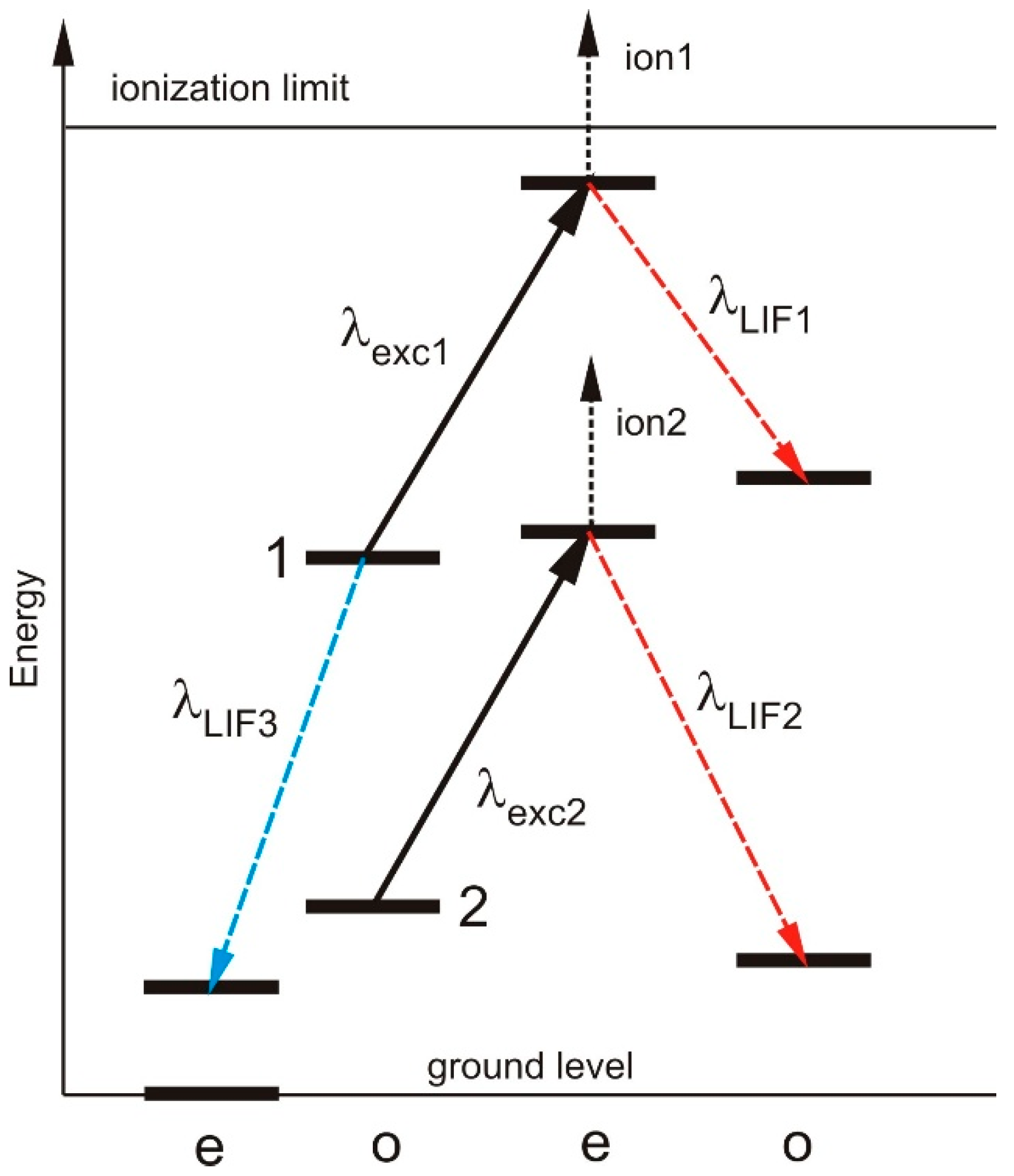
Due to excitation with intensity modulated laser light, the population of the lower level of the investigated transition is periodically lowered and the population of the upper level is periodically enhanced. (i) Thus, the fluorescence light emitted by the upper level of the transition is modulated and can be recorded by phase-sensitive detection (laser-induced fluorescence, LIF). Such transitions are called “positive” LIF-lines. (ii) The laser-excitation causes a decrease of the intensity of spectral lines for which the lower level of the laser transition decays to a very low-lying energy level. In this case the intensity of such lines is modulated with opposite phase relative to the exciting light, and we call it “negative” LIF-lines. Figure 1 shows the signals which may be observed due to LIF spectroscopy. A more detailed description one can find e.g., in [5].
Laser excitation of an atomic transition disturbs also the detailed equilibrium between excitation—and de-excitation processes in the discharge and therefore changes the impedance of the system. Thus, the current through the discharge can be used to monitor laser excitation and an optogalvanic (OG) signal can be observed. Instead of recording an OG signal, also the absorption of the laser light can be detected, as described e.g., in [6].
Using LIF, the additional information of the fluorescence wavelength can help to find which levels are involved in the excited transition. On the other hand, for finding new spectral lines this method is not suitable, one needs a method which is not sensitive to which levels are excited, like OG detection, or—without laser excitation—the emission spectrum of the discharge.
3. Finding of New Energy Levels by Laser Spectroscopy
New energy levels (in each emission spectrum one can find non-classified lines) can be found from emission spectra using the combination principle of Ritz or by laser spectroscopy, exciting unclassified lines. Here one has to solve the problem of finding suitable excitation wavelengths and use methods which allow to identify the levels involved in the excited transition.
3.1. Finding of Excitation Wavelengths
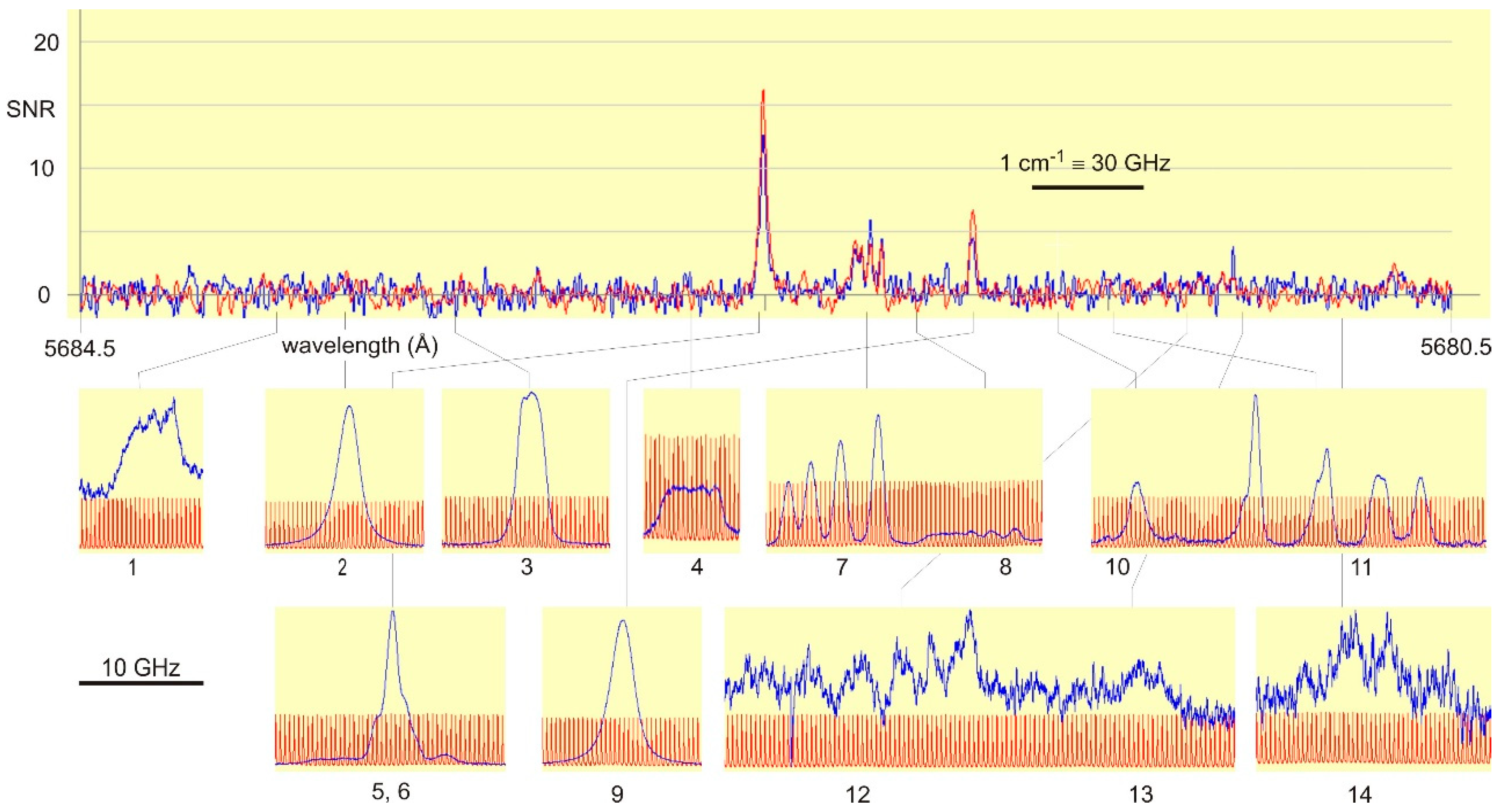
If unclassified spectral lines are given either in the wavelength tables of an element, or such lines are contained in emission spectra, such lines can be used to set the laser wavelength. A problem may be insufficient accuracy of photographically-determined wavelengths. FT spectra have very high wavelength precision, but weak lines usually are hidden in the noise of the spectra. Thus, in some cases, one has to search for unknown and unclassified lines by a laser-spectroscopic scan over a wide spectral range, using a non-state-selective detection method, like laser light absorption or OG spectroscopy. For La in my group such OG spectrum was recorded between the (for laser spectroscopy quite huge) range from 6200–5500 Å. A part of the OG spectrum, covering a range of 4 Å, is shown in Figure 2. In this range in the MIT tables [7] two Ar lines are listed at wavelengths 5683.73 and 5681.900 Å, and one structure belonging to La: 5681.1 Å with the remarks bh (band head of a molecule) and wh (wide and hazard, which means that the classification is not sure). Using OG spectroscopy, altogether 14 lines showed up, listed in Table 1. One can clearly see that, for La, the OG spectrum provides many more lines than known before. However, such an improvement is not achievable for all chemical elements and the method described here is not applicable for all of them.
While in commonly used wavelengths tables [7] only three lines are mentioned in the wavelength range of Figure 2, the OG spectrum shows—besides two Ar I-lines—altogether 12 previously unknown La I-lines as listed in Table 1. Two lines led to new levels as described here; three weak lines are still unclassified.
3.2. Setting Excitation Wavelength, e.g., to 5683.40 Å
The results of the systematic OG scan can now be used to set the excitation wavelength to the maximum of the OG signal of a line, which cannot be classified as transition between already known energy levels. As example, the results when setting the excitation wavelength to 5683.40 Å, are described.
3.3. Observation of LIF Signals, Location of a New Energy Level
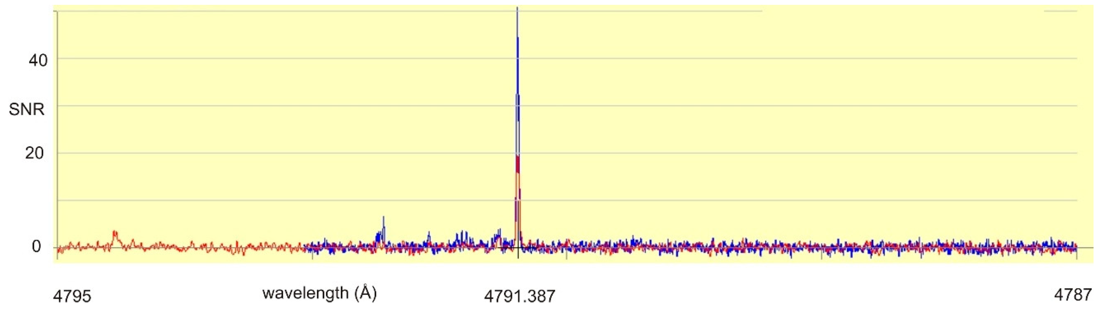
After setting the laser light wavelength, a search for LIF lines was performed, tuning the monochromator, which analyzes the light emitted by the discharge. A strong signal was found at 4792 ± 2 Å, having opposite phase compared to the excitation (“negative” LIF). When having a look at the FT spectrum in the neighborhood of 4792 Å, only one strong line at 4791.387 Å can be found (see Figure 3). This line is classified as transition between the odd-parity level at 23,874.946 cm−1, J = 5/2 and the even-parity level at 3009.993 cm−1, J = 5/2. Due to experience, such strong transitions between odd medium energy levels and low-lying even parity metastable levels show “negative” LIF signals. Thus, 23,874.946 cm−1 is assumed to be the lower level of the laser excitation.
A further need for finding a new level from this observation is (i) the correct classification of the line at 4791.387 Å and (ii) a check that it is really the line at which the LIF signal is observed. For a check, a transition list from the level at 23,874.946 cm−1 to lower levels is generated. In this list further possible “negative” LIF lines are contained. Indeed, LIF signals at 4714, 4381, and 4188 Å were observed, as well, confirming that 23,874.946 cm−1 is the really lower level of the excited transition.
Addition of the wave number of the excitation wavelength, 17,590.73 cm−1, gives the location of a new energy level at 41,465.17 cm−1, having even parity and a possible angular momentum J = 3/2, 5/2, or 7/2 (since 23,874.946 cm−1 has J = 5/2, and ΔJ = ± 1, 0 should hold).
3.4. Determination of Correct J-Value
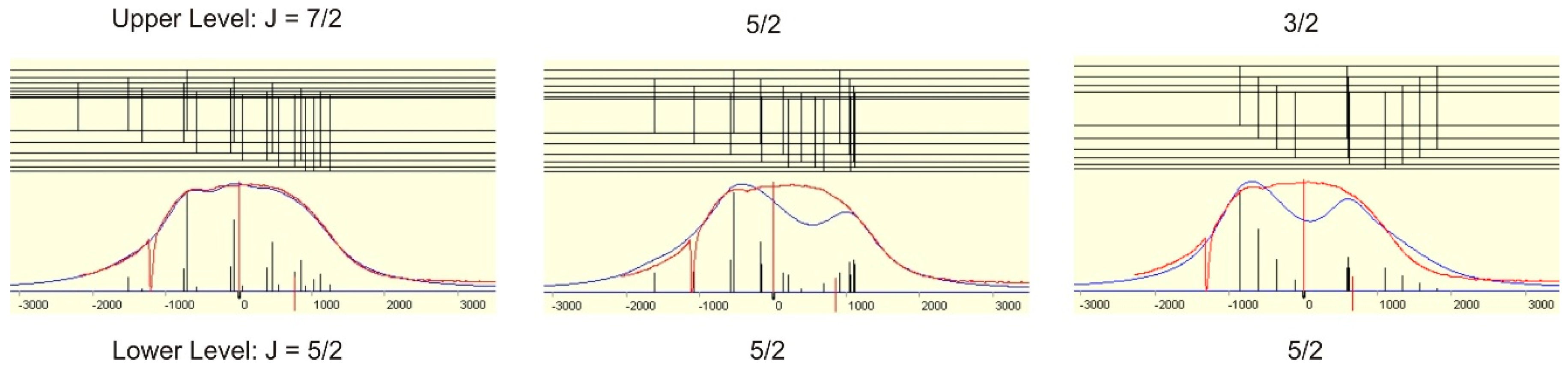
The correct J-value can either be proved by excitation of other lower levels having suited J-values or by the shape of the observed hf pattern. Since the hf constants of the level at 23,874,946 cm−1 are known from literature ([12], A = 241.7(2.3) MHz) simulation of the hf structure can be performed. In the present case, simulation is only possible if J = 7/2, A = 115(5) MHz (see Figure 4). If a simulation would not be possible with all three J-values, the assumed lower level would be the wrong one.
The hf constant of the lower level at 23,874.946 cm−1 (J = 5/2) was known from [12] to be 241.7(2.3) MHz. Only with J = 7/2 a simulation is possible. For this a FWHM of 900 MHz and Lorentzan line shape was assumed. The simulation gave A = 115(5) MHz.
3.5. Confirmation of the Existence of the New Level
First, the new even-parity level is added to the list of known La levels, including J = 7/2 and A = 115 MHz. Thus, the investigated line, wavelength 5683.40 Å, is now classified as the transition between a new level at 41,465.17 cm−1, J = 7/2, and the odd-parity level at 23,874.946 cm−1, J = 5/2.
Next, a list of transition wavelengths from the new level to other levels of odd parity (obtaining ΔJ = ± 1, 0) is calculated. Additional to the wavelength the hf pattern is predicted, but nothing can be said about transition probability. Thus, such calculated lines may not exist.
This list is compared with the entries of a database which contains all already observed La lines (from FT spectroscopy, laser spectroscopy, and wavelength tables). One can now look up if lines, unclassified up to now, are explained by the new level (if a highly-resolved FT spectrum or a laser spectroscopic gained spectrum is available, not only the wavelength but also the hf pattern must match).
If calculated wavelengths are in the range of available laser light sources one can try to laser-excite such lines. Since the calculated transition list also contains the combining levels, possible decays of these levels can serve as “negative” LIF lines, so one knows to which wavelength the monochromator must be tuned in order to get a confirming signal. In the present case, 12 excitations between 5500 and 6800 Å did finally lead to OG and/or LIF signals but, in principle, one additional excitation is enough to prove the existence. Among the 12 transitions the lower J-values vary between 9/2 and 5/2, confirming J = 7/2. The recorded hf patterns allowed a more precise determination of the hf constant A. From blend situations some transition wavelengths could be determined with higher precision as given by the lambdameter used in the experiments (accuracy ± 0.01 Å, limiting the energy value to ±0.05 cm−1), thus the energy of the new level could also be determined more precisely.
Finally, for the new even-parity level the values 41,465.181(10) cm−1, J = 7/2, A = 116(1) MHz are derived. Figure 5 shows the pattern on which the hf constant was finally determined, using a fit program called “Fitter” [13]. The wavelength of the line (no. 3 in Table 1) at which the level was discovered, is calculated to from the energy values to be 5683.395 Å, in very good agreement with the first assumed cg wavelength 5683.40 Å (resolution of the lambdameter 0.01 Å, position of the cg estimated).
In similar way excitation of the line no. 6, blended by the strong line no. 5 (numbers from Table 1) and having nearly the same cg wavelength, led to a new even-parity level at 41,681.502(10) cm−1, J = 5/2, A = 354(2) MHz. For both new levels the electric quadrupole constant B was assumed to be zero, since the quadrupole moment of the La nucleus is very small and the energy shift of the hf levels due to the influence of B are neglectible.
4. Conclusions
The example given above tells us which tools are necessary for the classification of a line and for the characterization of a new energy level:
- -
- list of all observed wavelengths in an extended spectral range;
- -
- exactly known excitation wavelengths (within the Doppler width), needed uncertainty ca. 0.01 Å;
- -
- from experiment: recording of hf pattern;
- -
- from experiment: finding of LIF lines and their relative phase;
- -
- reliable classification of LIF lines;
- -
- calculation of the energy of the new level;
- -
- simulation of the hf pattern to find J and A of the unknown level involved in the observed line;
- -
- calculation of a transition list from the new level to other known levels;
- -
- prediction of excitation wavelength, hf pattern, and LIF lines; and
- -
- from experiment: confirmation by laser excitation of calculated transition wavelengths.
All these tools are now available using the program “Elements”, described in [14,15]. In contrast to previous work a long time ago [16], now all the needed tools are available during the performance of the experiment, and usually immediately after finding a LIF line and recording of the hf pattern the new level can be found. Then, immediately, the existence of the level can be confirmed. Of course, there are also cases for which the procedure described is not so successful, e.g., if in the wavelength range of the available laser light no confirming excitation is successful. The program “Elements” is available for free from L.W. ([email protected]).
Funding
This research received no external funding.
Acknowledgments
First, I would like to mention all co-operations in the field of hf investigations, line classifications, and finding of new energy levels: G.H. Guthöhrlein, Helmut Schmidt-Universität Hamburg, Hamburg, Germany, and co-workers; J. Dembczynski, University of Technology, Poznan, Poland, and co-workers; J. Pickering, Imperial College London, UK; R. Engleman, University of New Mexico, Albuquerque, NM, USA; R. Ferber, University Riga, Latvia; E. Tiemann, University Hannover, Germany; J. Kwela, University Gdansk, Poland, and co-workers; S. Kröger, Hochschule für Technik und Wirtschaft Berlin, Berlin, Germany; G. Basar, University Istanbul, Turkey, and co-workers. Secondly, I appreciate the work of all the people who worked in Graz on this subject, especially C. Neureiter, B. Gamper and T. Binder, who helped in performing the experiments described in this paper. Finally, I would like to thank H. Jäger (head of the institute from 1975 to 1999) and W. Ernst (head of the institute from 2002 to present) for their continuous support.
Conflicts of Interest
The author declares no conflicts of interests.
References
- Moore, C.E. Atomic Energy Levels; Circular of the National Bureau of Standards 467; U.S. Government Printing Office: Washington, DC, USA, 1958; Volume III.
- Kramida, A.; Ralchenko, Y.; Reader, J.; NIST ASD Team. NIST Atomic Spectra Database (Version 5.3); National Institute of Standards and Technology: Gaithersburg, MD, USA, 2015. Available online: http://physics.nist.gov/asd (accessed on 30 June 2018).
- Windholz, L.; Gamper, B.; Binder, T. Variation of the observed widths of La I lines with the energy of the upper excited levels, demonstrated on previously unknown energy levels. Spectr. Anal. Rev. 2016, 4, 23–40. [Google Scholar] [CrossRef]
- Windholz, L.; Gamper, B.; Glowacki, P.; Dembczynski, J. The puzzle of the La I lines 6520.644 Å and 6519.869 Å. Spectr. Anal. Rev. 2014, 2, 10. [Google Scholar] [CrossRef]
- Mu, X.L.; Deng, L.H.; Huo, X.; Ye, J.; Windholz, L.; Wang, H.L. Hyperfine structure investigations in atomic iodine. J. Quant. Spectrosc. Radiat. Transf. 2018, 217, 229–234. [Google Scholar] [CrossRef]
- Martin, W.C.; Zalubas, R.; Hagan, L. Atomic Energy Levels—The Rare-Earth Elements; National Bureau of Standards NSRDS-NBS 60; US GPO: Washington, DC, USA, 1978.
- Harrison, G.R. Wavelength Tables; Massachusetts Institute of Technology, The MIT Press: Cambridge, MA, USA, 1969. [Google Scholar]
- Güzelçimen, F.; Başar, G.Ö.; Tamanis, M.; Kruzins, A.; Ferber, R.; Windholz, L.; Kröger, S. High-resolution Fourier transform spectroscopy of lanthanum in Ar discharge in the near infrared. Astrophys. Suppl. Ser. 2013, 218, 18. [Google Scholar] [CrossRef]
- Başar, G.Ö.; (Istanbul University). Personal communication, 2017. Level not yet published.
- Furmann, B.; Stefańska, D.; Dembczyński, J. Experimental investigations of the hyperfine structure in neutral La: II. Even parity levels. J. Phys. B 2010, 43, 015001. [Google Scholar] [CrossRef]
- Gamper, B. Hyperfine Structure Analysis of Praseodymium and Lanthanum. Ph.D. Thesis, Graz University of Technology, Graz, Austria, 2013. Unpublished. [Google Scholar]
- Furmann, B.; Stefańska, D.; Dembczyński, J. Hyperfine structure analysis odd configurations levels in neutral lanthanum: I. Experimental. Phys. Scr. 2007, 76, 264. [Google Scholar] [CrossRef]
- Guthöhrlein, G.H. Program Package “Fitter”; Helmut-Schmidt-Universität, Universität der Bundeswehr Hamburg: Hamburg, Germany, 1998; Unpublished. [Google Scholar]
- Windholz, L.; Guthöhrlein, G.H. Classification of Spectral Lines by Means of their Hyperfine Structure. Application to Ta I and Ta II Levels. Phys. Scr. 2003, T105, 55. [Google Scholar] [CrossRef]
- Windholz, L. Finding of previously unknown energy levels using Fourier-transform and laser spectroscopy. Phys. Scr. 2016, 91, 114003. [Google Scholar] [CrossRef]
- Guthöhrlein, G.H.; Mocnik, H.; Windholz, L. A new energy level of the neutral tantalum atom. Z. Phys. D 1995, 35, 177–178. [Google Scholar] [CrossRef]
Figure 1.
LIF signals which can be observed due to laser excitation. It is assumed that the excitation wavelengths 1 and 2 are closely neighbored, thus, a blend situation is observed with not state-selective detection (e.g., OG spectroscopy). When detecting positive LIF lines (shown in red), the upper level can be identified and—due to the different LIF wavelengths 1 and 2, the blend lines can be separated. The lower level of excitation 1 can be identified also by detecting LIF-line 3. Since the population of state 1 is lowered by laser excitation, the LIF signal 3 has opposite phase (“negative” LIF) compared to LIF-signals 1 and 2. If the upper level of transition 1 is close to the ionization limit, its ionization probability may be large, leading to a good OG signal but a decrease of the intensity of LIF-line 1, in some cases not distinguishable from noise. This situation is usually true for even La-levels with energies larger than 41,000 cm−1 (limit 44,981 cm−1 [3]). The observed linewidth is influenced by collisional broadening and can vary with the level energy (see [4]).

Figure 2.
Comparison of the available FT spectrum [8] (two overlapped spectra under different discharge conditions shown in red and blue) and optogalvanic spectra in the same wavelength range. In the OG spectra the red trace is the transmission signal of a marker etalon with free spectral range of 367.3 MHz. The OG spectra are normalized to the same amplitude, even their SNR is quite different.

Figure 3.
Fourier-transform spectrum in the wavelength range of the observed (“negative”) fluorescence line (4792 ± 2 Å). There is only one strong line, which can be classified as transition between an odd-parity level with medium energy (23,874.946 cm−1) and an even-parity metastable low-lying level (3009.993 cm−1). Due to experience, only intense lines of such type act as “negative” fluorescence lines.

Figure 4.
Simulation of the observed hf pattern of the line at 5683.40 Å assuming different values for the total angular momentum of the new fine structure level.
Figure 4.
Simulation of the observed hf pattern of the line at 5683.40 Å assuming different values for the total angular momentum of the new fine structure level.

Figure 5.
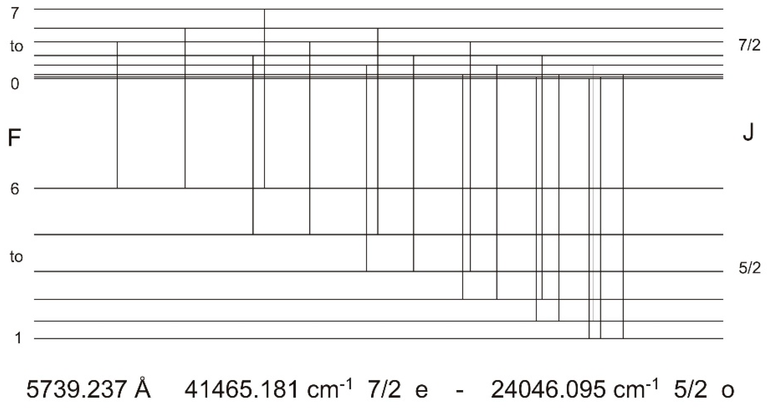
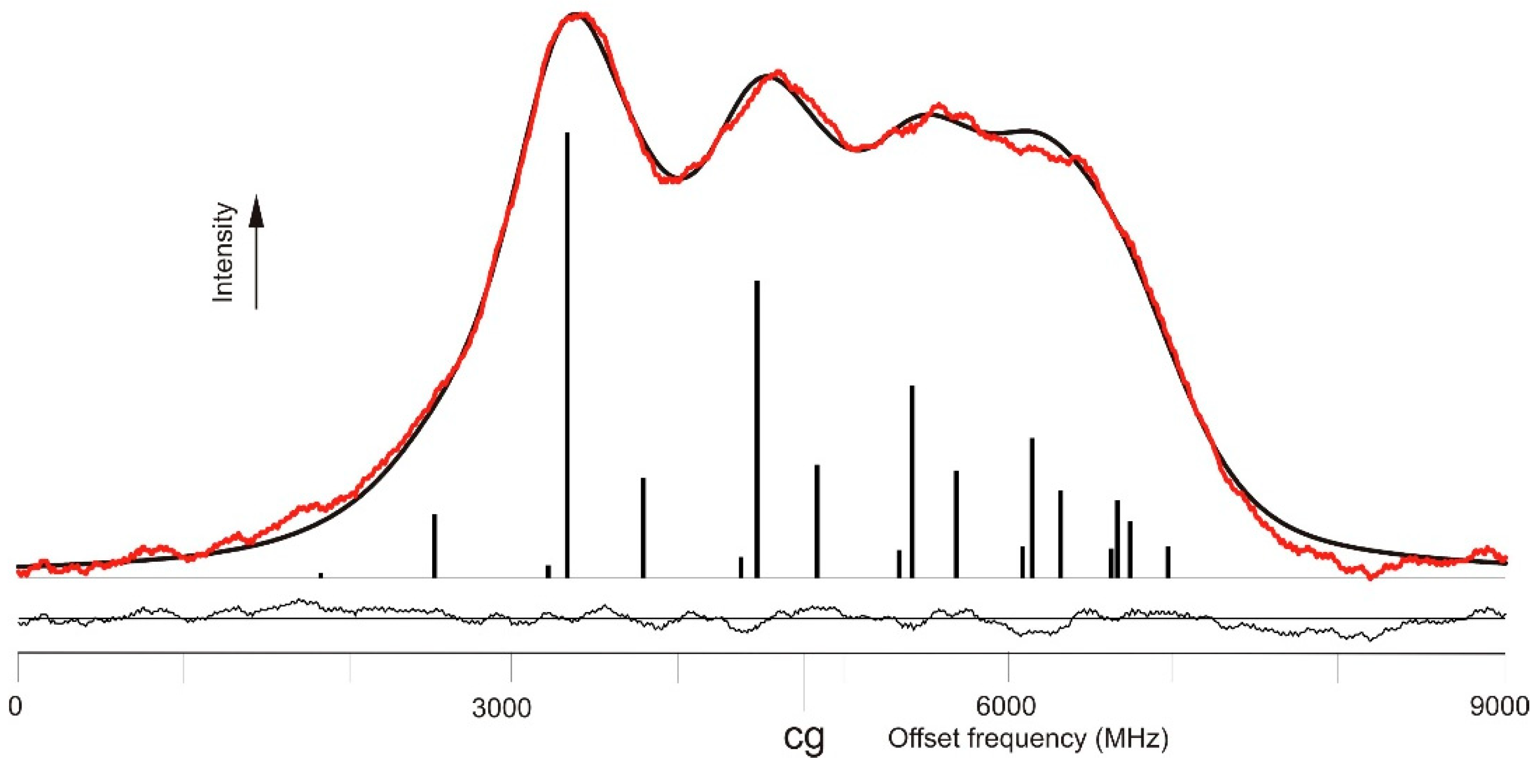
OG recorded hf pattern of the line at 5739.237 Å (transition between the new even level at 41,465.181 cm−1, J = 7/2, A = 116 MHz and a known odd lower level, 24,046.095 cm−1, J = 5/2, A = 325.8(17) MHz [12]), excited as confirmation of the existence of the newly found level. Red line: experiment; black line: fitted curve assuming a Voigt profile. The FWHM was fitted to be 900 MHz. Also shown is the hf level scheme and the position of the hf components and their intensities (theoretical ratios). The lower trace shows the residual between experimental and fitted curve. At this line a negative LIF signal at 4157 Å was observed, confirming that the lower level of this laser-excited transition is 24,046.095 cm−1.
Figure 5.
OG recorded hf pattern of the line at 5739.237 Å (transition between the new even level at 41,465.181 cm−1, J = 7/2, A = 116 MHz and a known odd lower level, 24,046.095 cm−1, J = 5/2, A = 325.8(17) MHz [12]), excited as confirmation of the existence of the newly found level. Red line: experiment; black line: fitted curve assuming a Voigt profile. The FWHM was fitted to be 900 MHz. Also shown is the hf level scheme and the position of the hf components and their intensities (theoretical ratios). The lower trace shows the residual between experimental and fitted curve. At this line a negative LIF signal at 4157 Å was observed, confirming that the lower level of this laser-excited transition is 24,046.095 cm−1.


Table 1.
Lines shown in Figure 2. nLIF: observation of a “negative” fluorescence line at the given wavelength (±2 Å). Wavelengths in column 2 are either determined from the FT spectrum or measured by the wavemeter. References for the energy levels are also given.
Table 1.
Lines shown in Figure 2. nLIF: observation of a “negative” fluorescence line at the given wavelength (±2 Å). Wavelengths in column 2 are either determined from the FT spectrum or measured by the wavemeter. References for the energy levels are also given.
| Line | Upper Level | Lower Level | Comment | |||||||
|---|---|---|---|---|---|---|---|---|---|---|
| no. | Wave-Length (Å) | Energy (cm−1) | J | P | Energy (cm−1) | J | P | |||
| 1 | 5683.94 | 40,392.82 * | 3/2 | e | [9] | 22,804.250 | 5/2 | o | [3] | * preliminary, not published |
| 2 | 5683.73 | 123,826.7500 | 2 | e | [2] | 106,237.5518 | 2 | o | [2] | Ar I |
| 3 | 5643.40 | 41,465.181 | 7/2 | e | this work | 23,874.946 | 5/2 | o | [2] | nLIF 4792 |
| 4 | 5682.72 | 40,813.42 | 7/2 | e | [10] | 23,221.097 | 7/2 | o | [3] | |
| 5 | 5682.507 | 31,688.660 | 3/2 | e | [3] | 14,095.677 | 1/2 | o | [3] | |
| 6 | 5682.51 | 41,681.502 | 5/2 | e | this work | 24,088.541 | 7/2 | o | [3] | nLIF 4337Blend with line 5 |
| 7 | 5682.196 | 37,612.922 | 3/2 | e | [3] | 20,018.977 | 3/2 | o | [3] | |
| 8 | 5682.08 | 38,566.480 | 7/2 | e | [10] | 20,972.166 | 5/2 | o | [3] | |
| 9 | 5681.896 | 123,832.4190 | 3 | e | [2] | 106,237.5518 | 2 | o | [2] | Ar I |
| 10 | 5681.67 | 41,300.404 | 1/2 | e | [11] | 23,704.816 | 3/2 | o | [3] | |
| 11 | 5681.50 | 35,393.395 | 5/2 | e | [3] | 17,797.301 | 3/2 | o | [3] | |
| 12 | 5681.22 | not classified | ||||||||
| 13 | 5681.11 | not classified | ||||||||
| 14 | 5680.80 | not classified | ||||||||
© 2018 by the author. Licensee MDPI, Basel, Switzerland. This article is an open access article distributed under the terms and conditions of the Creative Commons Attribution (CC BY) license (http://creativecommons.org/licenses/by/4.0/).
Share and Cite
MDPI and ACS Style
Windholz, L. Progress in Finding New Energy Levels Using Laser Spectroscopy. Atoms 2018, 6, 54. https://doi.org/10.3390/atoms6040054
AMA Style
Windholz L. Progress in Finding New Energy Levels Using Laser Spectroscopy. Atoms. 2018; 6(4):54. https://doi.org/10.3390/atoms6040054
Chicago/Turabian StyleWindholz, Laurentius. 2018. "Progress in Finding New Energy Levels Using Laser Spectroscopy" Atoms 6, no. 4: 54. https://doi.org/10.3390/atoms6040054
Note that from the first issue of 2016, this journal uses article numbers instead of page numbers. See further details here.