First Results of the “Carbonaceous Aerosol in Rome and Environs (CARE)” Experiment: Beyond Current Standards for PM₁₀

Abstract

In February 2017 the “Carbonaceous Aerosol in Rome and Environs (CARE)” experiment was carried out in downtown Rome to address the following specific questions: what is the color, size, composition, and toxicity of the carbonaceous aerosol in the Mediterranean urban background area of Rome? The motivation of this experiment is the lack of understanding of what aerosol types are responsible for the severe risks to human health posed by particulate matter (PM) pollution, and how carbonaceous aerosols influence radiative balance. Physicochemical properties of the carbonaceous aerosol were characterised, and relevant toxicological variables assessed. The aerosol characterisation includes: (i) measurements with high time resolution (min to 1–2 h) at a fixed location of black carbon (eBC), elemental carbon (EC), organic carbon (OC), particle number size distribution (0.008–10 $\mathsf{\mu }$m), major non refractory PM₁ components, elemental composition, wavelength-dependent optical properties, and atmospheric turbulence; (ii) 24-h measurements of PM₁₀ and PM_2.5 mass concentration, water soluble OC and brown carbon (BrC), and levoglucosan; (iii) mobile measurements of eBC and size distribution around the study area, with computational fluid dynamics modeling; (iv) characterisation of road dust emissions and their EC and OC content. The toxicological assessment includes: (i) preliminary evaluation of the potential impact of ultrafine particles on lung epithelia cells (cultured at the air liquid interface and directly exposed to particles); (ii) assessment of the oxidative stress induced by carbonaceous aerosols; (iii) assessment of particle size dependent number doses deposited in different regions of the human body; (iv) PAHs biomonitoring (from the participants into the mobile measurements). The first experimental results of the CARE experiment are presented in this paper. The objective here is to provide baseline levels of carbonaceous aerosols for Rome, and to address future research directions. First, we found that BC and EC mass concentration in Rome are larger than those measured in similar urban areas across Europe (the urban background mass concentration of eBC in Rome in winter being on average 2.6 ± 2.5 $\mathsf{\mu }$g · m${}^{-3}$, mean eBC at the peak level hour being 5.2 (95% CI = 5.0–5.5) $\mathsf{\mu }$g · m${}^{-3}$ ). Then, we discussed significant variations of carbonaceous aerosol properties occurring with time scales of minutes, and questioned on the data averaging period used in current air quality standard for PM${}_{10}$ (24-h). Third, we showed that the oxidative potential induced by aerosol depends on particle size and composition, the effects of toxicity being higher with lower mass concentrations and smaller particle size. Albeit this is a preliminary analysis, findings reinforce the need for an urgent update of existing air quality standards for PM${}_{10}$ and PM${}_{2.5}$ with regard to particle composition and size distribution, and data averaging period. Our results reinforce existing concerns about the toxicity of carbonaceous aerosols, support the existing evidence indicating that particle size distribution and composition may play a role in the generation of this toxicity, and remark the need to consider a shorter averaging period (<1 h) in these new standards.

1. Introduction

There is evidence that ambient particulate matter (PM${}_{10}$ and PM${}_{2.5}$) pollution poses severe risks to the human health [1,2,3,4,5,6,7,8,9,10]. This has led governments to adopt air quality standards for PM${}_{10}$ and PM${}_{2.5}$. PM${}_{10}$ is a heterogeneous mix of solid and liquid particles of different sizes (from few nanometers to 10 $\mathsf{\mu }$m) and different composition (including carbonaceous material, trace metals, crustal material, nitrates, sulfates, sea salt, ammonium). The specific aerosol types responsible for health effects, among those constituing PM${}_{10}$, remain uncertain, and no safe level for the exposure to PM${}_{10}$ and PM${}_{2.5}$ has been found [4]. This has sparked the debate over the need to update these standards.

The carbonaceous aerosol has been suspected to be more toxic than other PM${}_{10}$ constituents [2,4,7,11]. In their modeling exercise to assess the contribution of outdoor air pollution sources to premature mortality on a global scale, Lelieveld et al. [2] considered the carbonaceous PM${}_{2.5}$ as five times more toxic than inorganic particles. It is not clear if carbonaceous aerosol health effects are due either to its chemical composition (as elemental carbon particles or as carrier of other organic and inorganic chemicals) or to its physical properties (particle size, number and surface area) [1,3,4,7,8,9,10]. The carbonaceous aerosol is mainly found in submicron atmospheric aerosol particles, and most of these particles are in the ultrafine particle (UFP) size range (diameter less than 100 nm) [12]. Toxicology of UFPs is an emerging discipline because the size of these particles facilitates both adverse health effects in the lung and effects extending beyond the respiratory tract. Evidences have been found between short-term exposures to UFPs and the cardio-respiratory health (no matter what the particle composition is) [4]. Associations between ultrafine particles and the health of the central nervous system have also been reported. Inhaled ultrafine particles may translocate to the brain [13] where they can cause adverse impacts by inflammation and oxidative stress, which are common mechanisms similar to those acting in the lung [14,15]. Recent cross over studies on UFP and daily mortality in Europe, however, still show contrasting results and question the lack of a standardized protocol for UFP data collection [16].

The carbonaceous aerosol in the atmosphere comes as a complex mixture of aerosol types. Major components are black carbon (BC), organic aerosol (OA) or organic carbon (OC), and brown carbon (BrC). These are always internally or externally mixed with other components. BC and BrC are carbonaceous aerosols in their chemical composition, but are named after their light absorption properties: BC because it looks blackish, BrC because it looks brownish. The size of these particles span from a few nanometers to a few micrometers. Relevant microphysics (size, mixing state, number) constitute one of the greatest uncertainties in both models and observations [17]. Importantly, no reference method has been developed yet for measuring the carbonaceous aerosol. In particular, there is no an accepted standard to measure BC [18]. Thermal-optical methods combined to chemical methods have traditionally been used to measure EC and OC, although drawing a clear border between organic macro molecules of OC and small clusters of possibly amorphous EC is challenging [18]. Spectral optical methods have traditionally separated BC from the bulk aerosol, while more recently BrC has been connected to the wavelength dependence of light absorption [12]. Recent development of single-particle instruments capable of detecting BC (i.e., the single-particle soot photometer, SP2) has provided a method to obtain number size distributions and mixing state of refractory BC (rBC), although the particle size range is very limited (80–300 nm). Significant steps forward in the OA characterisation have been made in recent years thanks to the use of field-deployable, high-resolution, time-of-flight aerosol mass spectrometers [19].

Carbonaceous aerosol levels in Europe are still uncertain, and certainly largely variable across the different regions [20,21,22,23]. Cavalli et al. [22] suggested that the atmospheric concentrations of PM${}_{10}$ and PM${}_{2.5}$ carbonaceous constituents increase when moving from Scandinavia to Central Europe towards the Mediterranean. The Mediterranean basin, characterized by low cloudiness and high incoming solar radiation, is indeed an area of particular sensitivity as far as air pollution and climate change are concerned, e.g., [24]. Modeling results by Lelieveld et al. [2] show that the mortality linked to outdoor air pollution (mostly by PM${}_{2.5}$) in this region would definitely not be low, and that Italy would rank 18 among the countries with premature mortality by PM${}_{2.5}$ and O${}_3$ related diseases. As per Lelieveld et al. [2]’s results, land traffic would be one of the source categories responsible for the largest impact on mortality in the European Countries around the Mediterranean. In urban areas of Southern Europe the relative contribution to carbonaceous aerosol from vehicle exhaust could be more significant than that of other sources—e.g., biomass burning from domestic heating [21,23].

In this paper, we present first results of carbonaceous aerosol measurements carried out in February 2017 in Rome. The aim of this paper is to provide baseline levels of carbonaceous aerosols for the urban area of Rome reducing the assessment uncertainties of aerosol optical, chemical and microphysical properties, and to address future research and policy directions. Measurements were carried out in the framework of the experiment entitled “Carbonaceous Aerosol in Rome and Environs (CARE)”. As the present paper is the first of more detailed papers about the results of this experiment, here we briefly describe the general idea and methods of the whole project. The CARE experiment addresses the following specific question: what is the color, size, chemical identity, and toxicity of BC and BrC in the urban background of Rome? To this end, a robust dataset of optical–microphysical–chemical properties of the carbonaceous aerosol was collected, together with toxicological data to characterise relevant human health exposure. Different techniques for measuring carbonaceous aerosol properties were coupled with the aim to improve data reliability. Number size distribution (0.008–10 $\mathsf{\mu }$m), composition (EC, OC, and major components of nor-refractory PM${}_1$), mass concentration, and wavelength-dependent optical properties (BC and BrC) of the bulk aerosol were measured at a fixed location in the downtown Rome with high-time resolution (from 1-min to 2-h). 24-h measurements of PM${}_{10}$ and PM${}_{2.5}$ mass concentration, EC/OC, Water Soluble OC (WSOC), and water soluble BrC (WSBrC) and levoglucosan were carried out at the same site. Mobile measurements were carried out to assess the spatial gradients of BC particles near urban roadways and building surfaces, and the connections between these gradients and the atmospheric turbulence will be assessed through Computational fluid dynamics modelling (CFD). Typical road dust loadings and emission factors due to traffic resuspension for PM${}_{10}$ and EC/OC were quantified with the aim to obtain the chemical profile of road dust emissions (only thoracic fraction) to apply in receptor modelling to quantify road dust contribution to PM, OC and EC concentrations. The toxicological assessment included the preliminary evaluation of the potential impact of ultrafine particles on lung epithelia performed by directly exposing BEAS-2B cells to air pollution. Cells were cultured at the air liquid interface and exposed to particles by using the Culltex RFS-1 module. Finally, the oxidative potential associated with carbonaceous aerosols was assessed (2-h time resolution), particle size dependent number doses deposited in different regions of the human body was modeled, and biomonitoring of polyaromatic hydrocarbons (PAHs) was performed.

2. Materials and Methods

2.1. Measurement Site

Measurements were carried out in Rome (Italy) in the middle of the Mediterranean sea (Figure 1), from 27 January to 28 February 2017.

Measurements were carried out at an urban background site, located in the city center of Rome, in a garden (“San Sisto”). The garden is not open to the public. The site is situated in between three traffic roads which are 100–800 m away. In particular, the distance to the nearest heavily trafficked road is 115 m (Figure 1).

2.2. Equipment Deployment

Equipment used during the CARE 2017 experiment is summarized in

Table 1. Equipment deployed during the CARE experiment and relevant experimental setup (see Abbreviations list).

Instrument	Variable	Sampling Head	RH	Time Resolution	On/Off Line
MAAP	eBC	PM${}_{10}$	<30%	1 min	on-line
Aethalometer	eBC, AAE	PM${}_{10}$	<30%	1 min	on-line
Nephelometer	${\sigma }_s$	PM${}_{10}$	<30%	1 min	on-line
Field Sunset	EC, OC	PM${}_{2.5}$	ambient	2 h	on-line
ACSM	OA, SO${}_4^{2-}$, NH${}_4^{+}$, NO${}_3^{-}$, Chl${}^{-}$	PM${}_1$	<30%	30 min	on-line
PAS 2000	PAH		ambient	5 min	on-line
Streaker sampler	Elemental composition,${\sigma }_a$, AAE	PM10, PM$2.5$	ambient	1 h	off-line
Filter sampler	${\sigma }_a$, AAE, WSOC, WSBrC	PM$2.5$	ambient	24 h	off-line
MPSS	PNSD (8 $<d_m<$ 700 nm)	PM${}_{10}$	<30%	5 min	on-line
APS	PNSD (0.5 $<d_a<$ 20 $\mathsf{\mu }$m)	PM${}_{10}$	<30%	5 min	on-line
PILS	Oxidative stress		ambient	2 h	off-line
ALI	Toxicity of lung cells	PM${}_{1.5}$	ambient	24 h	off-line
Ultrasonic anemometer	WS, TKE,		ambient	10 Hz	on-line
Meteorological station	hWS, T, P, TSR, RH			1 s	on-line
PBL mixing monitor				1 h	on-line

, including relevant sampling conditions (e.g., relative humidity, sampling head, time resolution). The concept here was to deploy different measurement techniques (e.g., different measurement principles, different time resolution, different measurement strategy), and inter-compare data. The final objective was to both identify components and reduce biases inevitably included in the measurement.

Mobile measurements are described in Section 2.3.15. The fixed equipment was installed on board of two units parked into the San Sisto garden (the max distance between different instruments was less than 10 m). The ACSM, APS, AE33, MAAP, Nephelometer, SMPS, ALI system, streaker sampler and meteorological station were mounted on one van. The Sunset, PILS, Stability monitor were mounted on a different van. The PM${}_{2.5}$ sampler, ultrasonic anemometer, and PAS 2000 were mounted outside. The APS, AE33, MAAP, Nephelometer, SMPS, were connected to the same sampling line, having inner diameter = 16 mm, lenght = 4 m, flowrate = 16 lpm, Re < 2000. This sampling line was equipped with PM${}_{10}$ sampling head and a (large TROPOS-made) nafion drier. The ACSM used a different line equipped with PM${}_1$ sampling head and a (small) nafion drier. The ALI system used a very short sampling line (less than 1 m) located very close (less than 1 m) from the aerosol line. Instruments are described in more detail in Section 2.3.1.

2.3. Aerosol Measurements

2.3.1. Equivalent Black Carbon

The eBC mass concentration was obtained by:

• a Multi Angle Absorption Photometer (MAAP, Thermo Scientific™ (Waltham, MA, USA)),
• a 7 wavelenght (370, 470, 520, 590, 660, 880 and 950 nm) aethalometer (model A33, Magee scientific [25])

According to instrument manufacturer, the eBC mass concentration from AE-33 was obtained from measurements at $\lambda$ = 880 nm. Note that the mass absorption coefficient used from the manufacturer to obtain this eBC value is 7.77 m${}^2$· g${}^{-1}$ [25].

Only data in between the 1st and 99th percentiles were retained.

2.3.2. Aerosol Absorption Coefficients from Online Measurements

The absorption coefficient (${\sigma }_a$) at 637 nm was obtained from MAAP measurements after the following correction (Equation (1)):

$${\sigma }_a(637)=eBC·Q_{BC}·1.05$$

(1)

where eBC is the equivalent mass concentration of BC reported by the instrument, Q${}_{BC}$ = 6.6 m${}^2$· g${}^{-1}$ is the specific absorption coefficient of BC used in the firmware of MAAP, and the factor 1.05 accounts for a wrong wavelength during calibration experiments when determining Q${}_{BC}$ = 6.6 m${}^2$· g${}^{-1}$ [26]. This ${\sigma }_a$ was used to calculate the SSA.

To calculate the AAE of the bulk aerosol at 470–660 nm (AAE${}_{470-660}$), the ${\sigma }_a$ from AE33 at 470 and 660 nm were obtained by converting BC data provided by the AE33 with Mass absorption cross-section values indicated by the manufacturer (14.54 and 10.35 m${}^2$· g${}^{-1}$, respectively [25]).

2.3.3. Absorption Coefficients from Filter-Based Multi-$\lambda$ Polar Photometry

PM${}_{2.5}$ samples collected with 24-h resolution and streaker samples having 1-h resolution were measured by multi-$\lambda$ polar photometry at the Physics Department of the University of Milan (Italy) in order to retrieve absorption coefficients at four different wavelengths. The PP-UniMI polar photometer—a benchtop instrument developed by the Milan research group—was extensively described in [27,28] . Briefly, the instrument is based on the measurement on the scattering plane of the light transmitted and scattered in the forward and back hemispheres by unloaded and loaded samples using a photodiode mounted on a rotating arm. Data reduction aiming at the determination of the sample absorbance is performed according to [29] and literature cited therein. Currently, PP-UNIMI allows performing 4-$\lambda$ measurements (780, 635, 532, and 405 nm) on aerosol collected on different substrates, including high-time resolved samples obtained using a streaker sampler. The set-up of the instrument was validated against independent measurements carried out using a Multi-Angle Absorption Photometer (MAAP) for what concerns the red-light results, considering possible artefact effects shown in [27].

2.3.4. Scattering Coefficient

The dry scattering coefficient (${\sigma }_{\mathrm{s}}\left(\lambda \right)$) at 450, 525, and 635 nm was measured online with 1 min time resolution by an integrating nephelometer (Model Aurora 3000, Ecotech, Australia). Nephelometer data were corrected for truncation (Anderson and Ogren, 1998; Bond, 2001; Müller et al., 2011). The scattering error after the truncation error correction is $\frac{\delta ({\sigma }_{\mathrm{s}})}{{\sigma }_{\mathrm{s}}}=0$.02 [12]. The minimum detection limit of the nephelometer is 0.3 Mm${}^{-1}$, with calibration tolerance of ±4 Mm${}^{-1}$ and measurement range 0–2000 Mm${}^{-1}$.

2.3.5. OC/EC

The EC/OC mass concentration with 2-h time resolution was obtained by a Sunset Field Thermal-Optical Analyser (Sunset Laboratory Inc., Johannesburg, South Africa). Briefly, this instrument collects PM${}_{2.5}$ on a quartz fiber filter and automatically analyses it at the end of each sampling period. The instrument inlet is equipped with a cyclone (cut point 2.5 $\mathsf{\mu }$m) and an organic denuder. In this campaign, a time resolution of 2 h (105 min of sampling followed by 15 m of analysis) was chosen as a compromise to get an adequate time resolution (comparable with that of other instruments used in this project) and a sufficient amount of collected sample mass (to maintain a good accuracy in the EC-OC quantification). The instrument was calibrated by sucrose standards and the NIOSH protocol [30] was used for thermal analysis. Further, EC and OC were determined on 24-h quartz fiber filters by thermo-optical analysis with an offline OCEC Carbon Aerosol Analyser (Sunset Laboratory Inc., Johannesburg, South Africa) by applying the NIOSH-QUARTZ temperature protocol.

2.3.6. PM${}_{2.5}$ Sampler

Quartz-fiber filters were sampled with a PM${}_{2.5}$ sampler on a daily basis. Filters were first analysed for multi-wavelength optical absorption, and then cut and analysed for levoglucosan (1/4), water soluble BrC (3/8), and water soluble OC (3/8). This is described in the following sections.

2.3.7. Water Soluble OC

Water-soluble organic carbon (WSOC) was analysed on 24-h quartz fiber filters by TOC-VCSH (Shimadzu, Kyoto, Japan) by using the NPOC (non-purgeable organic carbon) procedure [31].

2.3.8. Water Soluble BrC

Light absorption spectra of water soluble carbon were measured off-line. Two 6 mm punches of quartz PM${}_{2.5}$ filters were extracted in 5 mL of ultrapure milli-Q water by 30 min ultrasonication. The extracts were filtered with 0.45 $\mathsf{\mu }$m cutoff PTFE syringe filters and analyzed, immediately after extraction, in parallel with blank filter samples. The UV-visible spectra were recorded with a TIDAS spectrometer coupled with a 0.5-m path length Liquid Waveguide Capillary Column (LWCC). The absorption coefficient of water soluble brown carbon (BrC) was calculated as the absorption at 365 nm, drift-corrected, and normalized by the volume of sampled air, according to the equation:

$$Ab{s}_{365}=(A365-A700)·\frac{V_e}{0.5·V_a}·ln(10)$$

(2)

A365 and A700 are the measured absorption at 365 and 700 nm, respectively, V${}_e$ is the extraction volume, V${}_s$ is the air sampling volume, 0.5 m is the optical path length. The wavelength of 365 nm is selected in order to reduce interference from inorganic species (i.e., nitrate) dissolved into water, and is comparable to previous literature studies [32,33].

2.3.9. Levoglucosan

For the determination of levoglucosan, 24-h quartz fiber filters were extracted in de-ionized water and the solution analysed by high-performance anion-exchange chromatography with pulsed amperometric detection (HPAEC-PAD), using a DC ICS-3000 oven, a GP40 gradient pump, a CarboPac™ PA10 analytical and guard column and a Dionex ED50/ED50A electrochemical cell. The same analytical method was used for the analysis of the solutions collected by the particle-into-liquid sampler (Section 2.5.4).

2.3.10. Elemental Composition by Streaker

Measurements for the determination of PM${}_{2.5}$ elemental composition with hourly resolution were performed at the INFN LABEC laboratory by means of Particle Induced X-ray Emission (PIXE) analysis. This technique is based on the detection and analysis of the X-rays emitted by the sample after excitation by an accelerated particle beam. PIXE allows the quantification of more than 20 elements with atomic number (Z) > 10 in a single measurement lasting only some tenths of seconds. This is a multi-elemental technique. With our set-up we simultaneously detect the X-rays of all the elements with Z > 10. In particular, we analysed the samples for the concentrations of: Na, Mg, Al, Si, P, S, Cl, K, Ca, Ti, V, Cr, Mn, Fe, Ni, Cu, Zn, As, Se, Br, Rb, Sr, Zr, Mo, Ba, Pb. Nevertheless, some elements (e.g., Rb, Zr, Mo…) were below detection limits in most cases.

Measurements were performed on samples collected with a streaker sampler [34] exploiting the external beam set-up fully dedicated to aerosol analysis available at LABEC. Details on the technique and the set-up, included the X-ray detection system, are given elsewhere [34,35]; here we briefly recall that the streak of collected particles is analysed point-by-point using a proton beam collimated in order to get a spot corresponding to 1-h sampling. Every point was measured for 60 s using a 300 nA beam; elemental concentrations were obtained via calibration relative to thin reference standards.

2.3.11. Non-Refractory PM${}_1$ Chemical Components

Major Non-refractory PM${}_1$ chemical components were measured using an Aerodyne Aerosol Chemical Speciation Monitor (ACSM). The ACSM is a mass spectrometer capable of analysing in real-time, with a temporal resolution of 30 min, the non-refractory at 600 °C component of the fine (<1 $\mathsf{\mu }$m) particulate (NR-PM${}_1$) [36]. The instrument analyses the mass spectrum of NR-PM1 by acquiring 100 different macromolecules (associated with pre-fixed mass-to-charge, $m/z$), providing the measurement of the main organic and inorganic chemical components: Organic matter (OA), sulfate (SO${}_4^{2-}$), ammonium (NH${}_4^{+}$), nitrate (NO${}_3^{-}$), Chloride (Cl${}^{-}$). For these technical features the ACSM allows, with respect to conventional measurement systems, (i) to have more information on the activity of the emission sources (variations within the daily cycle); (ii) to perform measurement campaigns also for limited periods; and (iii) to have a sufficient amount of data for application of multivariate statistical techniques that can contribute to the identification and quantification of the emission sources. The set of $m/z$ provides the mass spectra for speciation and quantification of the particulate air pollution main components; combinations of the obtained spectra’s time series can give information, after processing with multivariate analysis (Positive Matrix Factorization, PMF), to identify eventual chemically distinct groups of pollutants. The PMF analysis on the data of the organics permits the pre-identification of a number of factors (emission profiles) [37].

2.3.12. Polycyclic Aromatic Hydrocarbons

The EcoChem Photoelectric Aerosol Sensor (PAS) 2000 (PAS 2000 CE, EcoChem Analytics, Texas, and Matter Engineering AG, Switzerland) is a real-time monitor that measures the surface-associated total polycyclic aromatic hydrocarbons (PAHs) concentration . The PAS 2000 works on the principle of the photoionization of the particle-bound PAHs: the fine particles on whose surface PAHs are adsorbed are ionized by UV radiation, the charged particles are collected on a filter element and the resulting piezoelectric current is measured and proportionally related to the particle-bound PAHs. The logged data in 5 min intervals (expressed as total PAH concentration in $\mathsf{\mu }$g · m${}^{-3}$), were averaged over 30 min intervals for correlation with ACSM data.

2.3.13. Particle Number Size Distribution

The Particle number size distribution (PNSD) was measured by combining a Mobility Particle Size Spectrometer (TROPOS SMPS) equipped with a butanol-based condensation particle counter (CPC, TSI model 3772) and a commercial aerodynamic particle sizer (APS, TSI). Particles from 8 to 800 nm of electrical mobility diameter (d${}_m$) were sized and counted by the SMPS; particles from 0.5 to 20 $\mathsf{\mu }$m of aerodynamic diameter (d${}_a$) were sized and counted by the APS.

SMPS data were corrected for penetration errors through the sampling line (TROPOS-made software), penetration efficiency due to diffusion losses (calculated according to [38]) being higher than 98.92% for particles bigger than 15 nm.

APS aerodynamic diameters (d${}_a$) were converted to electrical mobility diameters (d${}_m$) as (Equation (3) [38]):

$$d_m=d_a·\sqrt{\frac{\chi ·{\rho }_0}{{\rho }_p}}$$

(3)

where ${\rho }_0$ is the reference density (1 g · cm${}^{-3}$); ${\rho }_p$ is the particle density; and $\chi$ is the shape factor. We assumed:

• size dependent effective particle density (${\rho }_p$) continuously varying from 1.6 to 2 g · cm${}^{-3}$ in the APS aerodynamic particle size range (cf. Figure S24 of the Supplementary materials);
• spherical particles ($\chi$ = 1);
• electrical mobility diameters (d${}_m$) representing the true particle diameter;
• Cunningham slip correction factor neglected in the APS size range.

To merge APS and SMPS, we used size distribution data expressed as $\frac{dN}{dlog(d_m)}$ similar to [39] (the $\frac{dN}{dlog(d_m)}$ distribution does not need a vertical shift, whereas the dN distribution does). The d${}_m$-based size distribution from APS (${(\frac{dN}{dlog(d_m)})}_{APS}$) was calculated as (Equation (4)):

$${(\frac{dN}{dlog(d_m)})}_{APS}={(\frac{dN}{dlog(d_a)})}_{APS}·\frac{dlog(d_a)}{dlog(d_m)}$$

(4)

Then, the ${(\frac{dN}{dlog(d_m)})}_{APS}$ were merged to relevant SMPS data (${(\frac{dN}{dlog(d_m)})}_{SMPS}$). The ${(\frac{dN}{dlog(d_m)})}_{SMPS}$ and ${(\frac{dN}{dlog(d_m)})}_{APS}$ overlapped for d${}_m$ from 475 to 830 nm (in fact, the first two channels of the APS were not used for the fitting procedure because of their unreliable counting and thus the overlapping size range was smaller). The ${(\frac{dN}{dlog(d_m)})}_{SMPS}$ were fitted with a power-law (Junge size distribution) function in this overlap size range (Equation (5)):

$${(\frac{dN}{dlog(d_m)})}_{fit}=C·d_m^{-\alpha }$$

(5)

An iterative procedure was used to estimate C and $\alpha$. A first guess-value is chosen and then varied based on the minimisation of the relative square difference between fitted and measured number size distributions at the two extreme particle diameters (Equations (6) and (7)):

$${(\frac{{\frac{dN}{dlog(d_m)}}_{fit}-\frac{dN}{dlog(d_m)}{)}_{APS}}{dlog{(d_m)}_{fit}})}^2$$

(6)

$${(\frac{{\frac{dN}{dlog(d_m)}}_{fit}-\frac{dN}{dlog(d_m)}{)}_{SMPS}}{dlog{(d_m)}_{fit}})}^2$$

(7)

Finally, the values of C = 1 and $\alpha$ = 4 ± 1 were used.

2.3.14. PM${}_x$

Daily PM${}_{10}$ and PM${}_{2.5}$ data were measured at a nearby urban background station (Arenula, 3 km from the CARE site) from the local environemntal agency (ARPA Lazio). Also, PM${}_1$ data were reconstructed from the BC and the NR-PM${}_1$ data.

In addition, PM${}_x$ data with 5 min resolution were reconstructed from the particle size distributions data measured by SMPS and APS, after the fitting procedure described in Section 2.3.13. A size dependent effective particle density was used (Figure S24 of the supplementary materials).

2.3.15. Mobile eBC Measurements

To determine the spatial variability of eBC mass concentration, parallel mobile measurements were performed using two TROPOS aerosol backpacks that measure concentrations of pollutants at a microscale level. Together with a GPS unit, data logger, and power supply, high time resolution, portable instruments that measure eBC (AE51) and particulate matter concentrations are placed inside a backpack, which can be carried by a single person.

Measurements or “runs” were done along a ∼9 km fixed route that includes different microenvironments to simulate different exposure scenarios. This route includes a 30-min stay at the fixed urban background station to ensure the data quality by comparing with the reference instruments for every run. Runs were performed three times a day (morning rush hour, afternoon, and evening) including weekends.

The data from the mobile measurements is the average of the two mobile instruments (AE51) running parallel to each other with a unit-to-unit variability of 0.068 $\mathsf{\mu }$g · m${}^{-3}$. The data from the reference fixed instrument were taken from MAAP at the fixed station representin the urban background concentration of eBC. MAAP measurements showed good agreement with the mobile instruments during the 30-min inter-comparison periods.

2.3.16. Road Dust Sampling

RD10 was collected at 10 sites around the S. Sisto area, around the CARE monitoring site, by means of a field resuspension sampler, consisting of a deposition chamber, an elutriation filter, where particles >10 $\mathsf{\mu }$m are separated, and a filter holder, where RD10 is collected [40]. Sites were chosen to represent highly trafficked sites and secondary residential streets. At each site, samples were collected following previous studies protocol [40,41]. Two filters were collected for each site, on the rightmost active lane. In some cases, sampling was performed on the curbside, therefore used only for the chemical profile. Before sampling, quartz fiber filters (Pall, 47 mm) were dried and conditioned before weighing; after sampling, filters were brought back to the laboratory for gravimetrical and chemical analyses [42]. Half of the sample was dissolved in acid (as in [42]) for the determination of major and trace elements by ICP-AES and ICP-MS, while another fraction was used for the determination of Organic and Elemental Carbon (OC and EC) by means of a Sunset Lab. ECOC analayzer using the EUSSAR2 protocol [43]. Pavement texture was analyzed by photographic analysis and by the Mean Texture Depth (MTD) analysis (ASTM E 965, 2015). Close-up photos of pavement surfaces were used to estimate average size of aggregates. Since aggregates are embedded in the asphalt binder, the surface macrostructure was also estimated by means of the MTD analysis [44]. The combination of the two analyses allowed obtaining the corrected aggregate median (CAM), according to the formula (Equation (8)):

$${\mathrm{CAM}}_i={\mathrm{MTD}}_i\times \frac{{(AggregateMedian)}_i}{{(AggregateMean)}_i}$$

(8)

where the mean and the median of the aggregates correspond to the values of the horizontal size of the aggregates observed in the photographic analysis.

2.4. Meteorological Measurements

Meteorological variables (temperature, relative humidity, pressure, wind) were measured by a standard meteo variables (Lufft weather station) with 1 min time resolution. As turbulence is a very important phenomenon affecting atmospheric processes near the surface, high frequency measurements of the three wind components u, v, w, and virtual temperature T${}_v$ were made with a Metek uSonic-3 Scientific thermo-anemometer (sampling frequency 10 Hz) installed 3.5 m a.g.l. From these measurements we computed the wind speed and direction as well as the fluctuations u${}^{\prime }$, v${}^{\prime }$, w${}^{\prime }$, and T${}_v$${}^{\prime }$ with respect to the 1-h linearly detrended mean wind components (ū, v̄, w̄) and virtual temperature (u${}^{\prime }$ = u − ū, v${}^{\prime }$ = v − v̄, w${}^{\prime }$ = w − w̄, $T_v$${}^{\prime }$ = $T_v$−${\overline{T}}_v$). We estimated the kinematic heat flux ($\overline{w^{\prime }{T}_v^{\prime }}$) and Turbulent Kinetic Energy (TKE) per unit mass (TKE/m = $\frac{1}{2}(u^2+v^2+w^2)$). The $\overline{w^{\prime }{T}_v^{\prime }}$ gives a measure of the thermal mixing capabilities of the atmosphere. The TKE represents the intensity of turbulence produced by fluid shear, friction or buoyancy, or through external forcing at low-frequency eddy scales. As both the $\overline{w^{\prime }{T}_v^{\prime }}$ and TKE vary significantly in time and in space, they need to be monitored during the all day.

Interesting additional information about the mixing properties of the lower atmosphere can be obtained by monitoring natural radioactivity due to Radon progeny [45,46,47]. During CARE, natural radioactivity was continuously measured on a 1-h basis. Natural radioactivity was measured by means of an automated monitor of Radon progeny (PBL Mixing Monitor, FAI Instruments, Fonte Nuova, Rome, Italy). The instruments detects natural radioactivity due to the decay products of Radon, a gas emitted from the ground at a rate that can be assumed to be constant on our observation scales (a few weeks, some kilometers). Radon undergoes radioactive decay only, and the concentration of its short-life decay products matches the time variations in the concentration of unreactive atmospheric pollutants emitted with a constant rate. Thus, the study of the time pattern of natural radioactivity allows an easy uncoupling of pollutants concentration variations that are due to changes in their emission/transformation rates from variations that are due to changes in the mixing properties of the lower atmosphere.

2.5. Toxicological Data

2.5.1. Air Liquid Interface (ALI) System

The human bronchial epithelial cell line BEAS-2B (ECACC, Salisbury, UK) were maintained in LHC-9 medium at 37 °C with 5% of CO${}_2$, split every three days. 72 h before exposure BEAS-2B were seeded on collagen coated transwell inserts (Corning Transwell^®, Corning Inc., New York, NY, USA) at a density of 15 × 10${}^3$ cells/insert. Then, the transwell were transferred into the CULTEX^® RFS Compact module (CULTEX Laboratories GmbH, Hannover, Germany) and the basal side of each chamber was filled with 4 mL of LHC-9 medium. The module was covered with a plastic seal and taken to the mobile lab for direct cell exposure. Cells were exposed at ALI to native atmosphere (insert at position 2, 4 and 6 of CULTEX^® RFS Compact) or to filtered air (negative controls at position 1, 3 and 5) for subsequent 24 h. Ambient air was sampled at 1.50 L/min, particulate matter bigger than 1.5 $\mathsf{\mu }$m was cut by a cyclone. 5 cm${}^3$· min${}^{-1}$ out of the 1.50 L/min sampled were used to expose each insert according to the geometry of the radial RFS-1 module. The number and mass of theoretical maximal deposited particles was than calculated according to [48].

2.5.2. Aerosol Dosimetry

Aerosol doses deposited into the human respiratory system have been estimated using the Multiple-Path Particle model Dosimetry (MPPD v3.01, ARA 2015, ARA, Arlington, VA, USA, [49]). The 60th percentile human stochastic lung was considered along with the following settings: (i) a uniformly expanding flow; (ii) an upright body orientation; and (iii) nasal breathing with a 0.5 inspiratory fraction and no pause fraction. Moreover, the following parameters were used for a Caucasian adult male under light work physical activity, based on the ICRP report [50]: (i) a functional residual capacity (FRC) of 3300 mL; (ii) an upper respiratory tract (URT) volume equal to 50 mL; (iii) a 20 min${}^{-1}$ breathing frequency; and (iv) an air volume inhaled during a single breath (tidal volume, VT) of 1.25 L.

2.5.3. PAHs Biomonitoring

Two of the researchers working on the project site, a man and a woman, collected urine samples for 15 consecutive days. Simultaneous quantitation of five urinary monohydroxylated metabolites of four polycyclic aromatic hydrocarbons (PAHs) was carried out using an HPLC-MS/MS analytical method: 1-hydroxypyrene (1-OHPy), 1-hydroxynaphthalene (1-OHNAP), 2-hydroxynaphthalene (2-OHNAP), 3-hydroxybenzo[a]pyrene (3-OHBaPy), 6-hydroxynitropyrene (6-OHNPy) [51]. Results were normalized for the creatininuria.

2.5.4. Oxidative Potential

A particle-into-liquid sampler (PILS) was used for on-line measurement of the oxidative potential (OP). The same system was used for levoglucosan measurements. The air flow is denuded from gaseous species, while aerosol particles are grown in a saturated water vapor chamber to form droplets. These are collected by inertial impact on a collection plate, washed by deionized water. The resulting solution was collected every 2 h for subsequent analyses [47].

The OP was determined by the 2’ 7’-dichlorofluorescein (DCFH) essay [52]. The OP is considered as a proxy of the ability of PM${}_x$ to generate reactive oxygen species (ROS, or free radicals) and is defined as the capacity of PM${}_x$ to oxidize target molecules. Different assays refer to different target molecules and are expected to lead to different OP values. In this work we used the 2’,7’-dichlorofluorescein (DCFH) assay. This assay was formerly developed for the in vitro determination of ROS in biological cells (e.g., [53]). In recent years, it has been adapted and applied as an acellular method (e.g., [54]). In this assay, the non-fluorescent DCFH is oxidized to the fluorescent dichlorofluorescein (DCF) in the presence of horseradish peroxidase (HRP).

3. Results

Here we present preliminary results of the CARE experiment. First, an overview of aerosol and meteorology data is given in Section 3.1. Then, aerosol characteristics are presented in Section 3.2. Third, toxicological results are presented in Section 3.3. These results are discussed in Secion Section 4.

3.1. Overview of Aerosol and Meteorology Data

Figure 2 shows the time series of the major carbonaceous aerosol features ( mass concentration of eBC and non-refractory PM${}_1$ components, spectral aerosol light absorption, and particle number size distribution, described in detail in the following subsections), with relevant meteorological and micro-meteorological parameters (wind speed and direction, friction velocity and Turbulent Kinetic Energy (TKE), temperature and sensible heat flux ($\overline{w^{\prime }{T}_v^{\prime }}$)). A statistical summary of these data is presented in

Table 2. Statistical summary of variables acquired from 16:00 2 February to 10:00 28 February 2017. Data are mean, median, standard deviation, minimum and maximum, 95% confidence interval (lower–upper), number of datapoints (#), and time resolution of data used to calculate the statistics (TR).

Variables	Mean	Median	st.dev.	Min–Max	95 % CI [mean]	#	TR
eBC ($\mathsf{\mu }$g · m${}^{-3}$)
MAAP	2.6	1.7	2.5	0.2–14.4	2.3–2.8	35,256	1 min
MAAP	2.7	1.6	2.6	0.5–9.9	2.5–2.9	609	1 h
MAAP	2.5	1.7	2.1	0.3–13.9	2.3–2.8	287	2 h
AETH	2.9	1.9	2.8	0.3–16.0	2.9–3.0	35,839	1 min
EC ($\mathsf{\mu }$g · m${}^{-3}$)	2.1	1.9	1.4	0.3–10.7	1.9–2.3	302	2 h
	2.2	2.1	1.1	0.6–4.6	1.7–2.6	26	24 h
MAC (m${}^2$ · g${}^{-1}$)
637 (MAAP,Sunset)	8.6	8.4	0.9	6.7–12.0	8.5–8.7	297	2 h
OC ($\mathsf{\mu }$g · m${}^{-3}$)
ACSM	7.8	5.0	6.8	0.01–32.5	7.4–8.2	1135	30 min
sunset	5.6	4.3	4.0	0.7–18.1	5.2–6.1	308	2 h
NR-PM${}_1$ ($\mathsf{\mu }$g · m${}^{-3}$, ACSM)
total mass	13	9	10	0–50	13–14	1135	30 min
NO${}_3^{-}$	2.75	1.41	2.86	0.07–14.3	2.58–2.92	1135	30 min
NH${}_4^{+}$	1.60	1.41	1.15	0.00–6.54	1.53–1.65	1004	30 min
SO${}_4^{-}$	1.30	1.15	0.90	0.00–3.72	1.25–1.36	1122	30 min
Cl${}^{-}$	0.17	0.09	0.32	0.00–6.29	0.15–0.19	942	30 min
PM${}_1$ ($\mathsf{\mu }$g · m${}^{-3}$)
ACSM+MAAP	16	11	12	2–54	14–17	287	2 h
SMPS+APS	16	11	11	2–47	14–17	290	2 h
PM${}_{2.5}$ ($\mathsf{\mu }$g · m${}^{-3}$)
Beta	17	16	7	6–32	14–20	25	24 h
SMPS + APS	18	15	11	3–51	17–20	279	2 h
PM${}_{10}$ ($\mathsf{\mu }$g · m${}^{-3}$)
Beta	26	27	9	9–45	22–30	24	24 h
SMPS+APS	24	23	14	2–67	22–26	280	2 h
BC/PM${}_{10}$	0.10	0.10	0.04	0.02–0.25	0.09–0.11	274
BC/PM${}_{2.5}$	0.13	0.12	0.06	0.03–0.41	0.13–0.14	274
BC/PM${}_1$	0.15	0.15	0.06	0.07–0.50	0.15–0.17	287
PAHs (ng · m${}^{-3}$)	24	11	33	0–252	21–26	951
N${}_{tot}$ $·{10}^3$ (cm${}^{-3}$)	12.3	11.0	7.7	0.1–40.9	12.1–12.5	7412	5 min
N${}_{tot}$ $·{10}^3$ (cm${}^{-3}$)	13.0	11.5	6.9	2.9–38.6	12.3–12.9	299	2 h
d${}_{med(S)}$ (nm)	81	86	23	10–115	80–81	7483	5 min
${\sigma }_{ap}$ (Mm${}^{-1}$)
405 (streaker)	25.1	15.3	26.3	5.9–180.4	23.0–27.1	628	1 h
532 (streaker)	19.2	11.4	20.7	2.5–147.2	17.6–20.86	628	1 h
635 (streaker)	16.24	9.74	17.84	3.4–123.26	14.86–17.66	628	1 h
637 nm (MAAP)	19.7	11.57	20.97	0.3–202.6	18.8–19.7	7300	5 min
780 (streaker)	13.5	7.2	15.3	3.4–104.0	12.3–14.7	628	1 h
${\sigma }_{sp}$ (Mm${}^{-1}$)
520 nm (Neph)	77.7	61.1	53.2	10.3–262.9		35,727	1 min
635 nm (Neph)	62.2	52.6	40.7	9.2–204.5		35,727	1 min
SSA
637 nm (Neph + MAAP)	0.778	0.796	0.105	0.278–0.969	0.776–0.781	7196	5 min
AAE
450–660 (AETH)	1.41	1.38	0.21	0.99–2.03	1.40–1.41	35,935	1 min
WS (m · s${}^{-1}$)	0.9	0.6	0.8	0.1–4.5	0.90–0.96	4032	1 min
TKE (m${}^2$ · s${}^{-2}$)	0.34	0.11	0.49	0.00–3.39	0.33–0.36	4032	1 min
T (C)	11.3	11.6	3.4	2.5–18.8		37,388	1 min
RH (%)	75	77	14	25–98		37,388	1 min
P (hPa)	1016	1017	780	919–1032		37,388	1 min

.

The Heat Flux ($\overline{w^{\prime }{T}_v^{\prime }}$) shows thermal mixing capabilities of the atmosphere, whereas the TKE the intensity of turbulence produced by fluid shear, friction or buoyancy, or through external forcing at low-frequency eddy scales (Section 2.4). Similar information on the mixing properties of the lower atmosphere were obtained by measuring the natural radioactivity due to Radon progeny (Section 2.4, Figures S23 and S24 of the Supplementary materials).

The presence and altitude of Saharan dust plumes have been determined on the basis of polarization-sensitive Lidar-ceilometer (PLC) observations and verified against model forecasts (e.g., www.diapason-life.eu). The relevant near-real time atmospheric profiling was made by means of the PLC system located in central Rome (data available at http://www.alice-net.eu/, “downtown Rome” site). In these measurements, suspended mineral dust is revealed by a sharp increase in the depolarization signal, i.e., the cross over the parallel polarized backscattered signals (an example is Figure S27 of the Supplementary materials). During CARE, Saharan dust layers were observed in the periods 3–6, 8–10, 18 and 24–28 of February 2017. Dust was observed to reach the ground in the last two periods only.

During the first days of the campaign (days 1–6), aerosol concentrations were lower due to bad weather conditions (Figure 2): strong winds from E-SE, high values of the momentum fluxes and TKE, low Radon concentrations (Figure S24 of the supplementary materials) and some showers (Figure S28 of the supplementary materials). Bad weather conditions also occurred on February 18–19 and 24–26 (i.e., days of Saharan dust advection). During the central period of the campaign (days 10–24, excluding the above mentioned days 18–19) the weather conditions were fairly stable. These conditions favoured the increase of aerosol mass concentrations (Figure 2). The typical local winter circulation prevailed, the peak of the wind speed (mostly below 2 m · s${}^{-1}$ at 12 LT) being due to the inland penetration of weak sea breezes.

A large variability of aerosol properties can be observed during the four weekends (WE) of the field measurements (Figure 2). This variability reflects in part the different conditions above mentioned. On the second weekend only (11–12 February 2017), fairly stable weather conditions occurred: the highest weekend concentrations were measured. On the first weekend (4–5 February 2017), third weekend (18–19 February 2017), and fourth weekend (25–26 February 2017), bad weather conditions occurred, instead: we measured lower concentrations, but different aerosol properties (e.g., the AAE). Differences may be explained as follows: (i) on the third weekend only, there was no Saharan dust advection; and (ii) on the fourth weekend only, a ban on private car traffic was introduced in downtown Rome (including the CARE measurement site), and an episode of wood burning occurred.

Figure 3 shows (a) the wind speed distribution and (b) the integrated eBC mass concentration for different wind angular sectors.

The distribution shows three major features: strong winds from E-SE, moderate winds from W-NW, and low winds which may occur from all directions (Figure 3a). As expected the higher the wind speed, the lower the eBC mass concentration (Figure 3 cf. Figure S8 of the supplementary materials). Conversely, higher concentrations are found for lower wind speeds from all angular sectors (i.e., around the source—both dusty and non dusty days show this tendency, Figure S7 of the supplementary materials). In Figure S9 of the supplementary materials, we show a dependence of eBC on the inverse of Monin Obukhov length (z/L), whereas in Figure S25 we show the relevant time series. The z/L is the ratio of the height of the sonic anemometer sensor (z = 3 m) to the Obukhov length (L), defined as (Equation (9)):

$$\mathrm{L}=\frac{u_{\ast }^3·\overline{T_v^{\prime }}}{k·g·(\overline{w^{\prime }{T}_v^{\prime }})}$$

(9)

where $u_{\ast }$ is the frictional velocity, $\overline{T_v^{\prime }}$ is the mean virtual potential temperature, $\overline{w^{\prime }{T}_v^{\prime }}$ is the Heat flux (i.e., surface virtual potential temperature flux), k is the von Kármán constant, and g is the gravitational acceleration. The absolute value of L indicates the height to which the convective turbulence (due to the buoyancy) begins to prevail over the turbulence due to the mechanical production (mainly due to the wind shear). The sign of L depends on the sign of the heat flux ($\overline{w^{\prime }{T}_v^{\prime }}$) only (all the other quantities are always > 0): (i) under convective conditions (heat flux > 0) L is negative; (ii) under stable conditions (heat flux < 0) L is positive; (iii) under the neutral condition (heat flux = 0) L = 0. The dependence between eBC and z/L (Figures S9 and S25) indicates that higher eBC concentrations occurred during stable to neutral atmospheric conditions, corresponding both to larger emissions and lower turbulent mixing.

3.2. Aerosol Characterisation

Figure 4 presents diurnal and weekly cycles of carbonaceous aerosol properties (mass and number concentrations, optical variables, and major sources).

Aerosol properties show clear diurnal and weekly cycles. A statistical summary of all data is given in Table 2.

Table 3. Temporal variability of major variables acquired between 2 February 16.00 and 28 February 10:00 2017 at the Rome site, separately shown for (case i) the morning rush hour (08:00 local time) of the working days, (case ii) evening peak (21:00) of the working days, and (case iii) weekends at midday (15:00). Data are presented as mean values and mean 95% confidence internal, relative number of datapoints used in the statistics (counts), and time resolution of data used to calculate the statistics (TR) being indicated.

Variables	Case	Mean (95 % CI)	Counts	TR
eBC ($\mathsf{\mu }$g · m${}^{-3}$)	(i)	3.9 (3.7–4.0)	962	1 min
	(i)	3.7 (3.2–4.2)	60	1 h
	(ii)	5.2 (5.0–5.5)	472	1 min
	(ii)	5.4 (4.7–6.0)	74	1 h
	(iii)	1.0 (1.0–1.0)	996	1 min
	(iii)	1.2 (1.1–1.3)	41	1 h
MAC637 (m${}^2$ · g${}^{-1}$)	(i)	8.9 (8.6–9.2)	33	2 h
	(ii)	9.3 (8.2 –10.3)	8	2 h
	(iii)	9.1 (8.6–9.5)	16	2 h
OA ($\mathsf{\mu }$g · m${}^{-3}$)	(i)	10.3 (7.8–12.8)	35	30 min
	(ii)	12.4 (10.0–14.8)	33	30 min
	(iii)	2.7 (1.6–3.7)	13	30 min
NO${}_3$ ($\mathsf{\mu }$g · m${}^{-3}$)	(i)	5.0 (3.7–6.3)	35	30 min
	(ii)	3.3 (2.5–3.3)	33	30 min
	(iii)	0.6 (0.3–0.8)	13	30 min
NH${}_4$ ($\mathsf{\mu }$g · m${}^{-3}$)	(i)	2.0 (1.5–2.4)	35	30 min
	(ii)	1.8 (1.4–2.3)	33	30 min
	(iii)	0.6 (0.7–0.9)	13	30 min
SO${}_4$ ($\mathsf{\mu }$g · m${}^{-3}$)	(i)	1.6 (1.2–1.9)	35	30 min
	(ii)	1.6 (1.3–1.9)	33	30 min
	(iii)	0.6 (0.4–0.9)	13	30 min
NR-PM${}_1$ ($\mathsf{\mu }$g · m${}^{-3}$)	(i)	19 (15–23)	35	30 min
	(ii)	20 (16–23)	33	30 min
	(iii)	4 (3–6)	13	30 min
PM${}_1$ ($\mathsf{\mu }$g · m${}^{-3}$)	(i)	21 (14–28)	15	2 h
	(ii)	23 (17–28)	16	2 h
	(iii)	5 (4–6)	8	2 h
PM${}_{10}$ ($\mathsf{\mu }$g · m${}^{-3}$)	(i)	29 (21–36)	15	2 h
	(ii)	35 (28–43)	16	2 h
	(iii)	14 (5–22)	8	2 h
eBC/PM${}_1$	(i)	0.20 (0.16–0.24)	16	2 h
	(ii)	0.19 (0.15–0.22)	16	2 h
	(iii)	0.13 (0.11–0.16)	8	2 h
eBC/PM${}_{10}$	(i)	0.14 (0.11–0.16)	15	2 h
	(ii)	0.11 (0.09–0.14)	15	2 h
	(iii)	0.07 (0.04–0.09)	8	2 h
N${}_{tot}$ (cm${}^{-3}$)	(i)	20.5 (19.3–21.6) $·{10}^3$	197	5 min
	(ii)	17.6 (16.1–19.1) $·{10}^3$	177	5 min
	(iii)	7.9 (7.0–8.8) $·{10}^3$	96	5 min
d${}_{med(S)}$ (nm)	(i)	80.0 (77.8–82.2)	207	5 min
	(i)	85.6 (84.2–87.0)	198	5 min
	(i)	73.8 (70.3–77.4)	96	5 min
SSA 635	(i)	0.702 (0.686–0.718)	203	1 min
	(ii)	0.716 (0.699–0.733)	214	1 min
	(iii)	0.843 (0.831–0.855)	96	1 min
AAE 470–660	(i)	1.32 (1.31–1.33)		1 min
	(ii)	1.39 (1.38–1.41)	471	1 min
	(iii)	1.29 (1.28–1.30)	996	1 min

presents a statistical summary of data measured during three case-study periods: the morning rush hour of the working days, the evening peak of the working days, and on the weekends at midday. All aerosol properties are presented in more details in the following paragraphs.

3.2.1. Black and Elemental Carbon

Different measurement techniques were coupled to obtain a robust estimate of BC and EC (Section 2.3.1). Data measured with different techniques show good correlations (r${}^2>$ 0.98, p< 0.001). However, the eBC and EC mass concentration differs widely from one measurement technique to another (Table 2). Figures S1–S4 of the supplementary materials show relevant results of the linear regression analysis.

The eBC mass concentration from MAAP (2.6 ± 2.5 $\mathsf{\mu }$g · m${}^{-3}$) is lower than the eBC mass concentration from AE-33 (2.9 ± 2.8 $\mathsf{\mu }$g · m${}^{-3}$). Note that the mass absorption coefficient used from the manufacturer to obtain this eBC value is 7.77 m${}^2$· g${}^{-1}$ [25], lower than the site specific MAC obtained during CARE (Section 3.2.2). The linear regression analysis coefficient (i.e., the slope of the regression line) is 1.11 (Figure S1). The eBC mass concentrations from MAAP and AE-33 are both higher than the EC mass concentration from 2-h Sunset (2.1 ± 1.4 $\mathsf{\mu }$g · m${}^{-3}$), the linear regression analysis coefficient of 1.19 and 1.35, respectively (Figures S3 and S4).

Regardless of the instrument used, the eBC mass concentration shows a clear diurnal variability with higher values at the rush hours and large differences between weekdays and weekends (Figure 4a—note that all Figures show eBC mass concentration from MAAP, unless otherwise specified). These differences are particularly evident at the morning rush hour (7.00–10.00 h, local time) when the mean value during the working-days is 3.9 (95% CI = 3.7–4.0) $\mathsf{\mu }$g · m${}^{-3}$ (Table 3). The highest eBC mass concentration is measured at the evening rush hour (20.00–1.00 h), with mean value of 5.2 (95% CI = 5.0–5.5) $\mathsf{\mu }$g · m${}^{-3}$. The lowest eBC mass concentration is observed during the central part of the day (14.00–16.00) of the weekends, the mean value being 1.0 $\mathsf{\mu }$g · m${}^{-3}$.

3.2.2. Mass Absorption Coefficient

The Mass Absorption Coefficient of BC in the aerosol (MAC${}_{BC}$)—a fundamental input for radiative trasfer models—was calculated as (Equation (10)):

$${\mathrm{MAC}}_{BC}(\lambda )=\frac{{\sigma }_a(\lambda )}{EC}$$

(10)

where $\lambda$ = 637 nm, EC is the mass concentration from 2-h Sunset, and ${\sigma }_a$ is the absorption coefficient from MAAP after the correction indicated in Equation (1). Site-specific MAC was estimated by the linear regression analysis of ${\sigma }_a(637)$ and EC (r${}^2$ = 0.994, p< 0.001, n = 297, Figure S10 of the Supplementary materials). Estimated this way, the average MAC${}_{BC}$ at 637 nm was 8.7 m${}^2$· g${}^{-1}$ (Std Error = 0.046). Also, MAC${}_{BC}$ at 637 nm was estimated as point-to-point ratio of ${\sigma }_a$ to EC (panel d of Figure 4), the mean value being 8.6 (95% CI = 8.5–8.7) m${}^2$· g${}^{-1}$. Larger values were observed at the evening rush hour and during week-ends (Table 3). Future research will analyse major factors govering MAC${}_{BC}$ variability.

Importantly, the use of this site-specific MAC${}_{BC}$ value clearly reduces the discrepancy between eBC mass concentration values obtained from AE-33 and MAAP.

3.2.3. Absorption Ångström Exponent

The Absorption Ångström Exponent (AAE) describes the wavelength ($\lambda$) dependence of the light absorption coefficient by aerosol (${\sigma }_a$) calculated as (Equation (11)):

$$\mathrm{AAE}(\lambda )=-\frac{dln({\sigma }_a)}{dln(\lambda )}$$

(11)

The AAE of the bulk aerosol obtained from AE-33 aethalometer (Section 2.3.2) is presented in Figure 2a (as data color code), daily and weekly cycles in Figure 4h. The AAE of the bulk aerosol at 470–660 nm (AAE${}_{470-660}$) was 1.41 ± 0.21, and varied from 0.99 and 2.03 (Table 2). This indicates a significant influence of primarily emitted BC at the site, as well as that traffic was not the only source. Lower AAE${}_{470-660}$ occurred at the rush hours of the working days (AAE${}_{450-660}$ of about 1.3, Table 3). Larger AAE${}_{470-660}$ values occurred during the night (01.00–5.00, and correspond to larger values of OA and aerosol size and lower values of the EC-to-OC ratios (Figure 4b,e,f). Future research will analyse this correspondence corroborating previous results which have indicated the strong dependence of AAE on both aerosol size and composition [12,55,56,57,58,59].

3.2.4. Single Scattering Albedo

The Single Scattering Albedo (SSA) is a key parameter to understand the fraction of aerosol light extinction due to absorption, and thus to evaluate aerosol warming or cooling effect. SSA is calculated as (Equation (12)):

$$\mathrm{SSA}(\lambda )=\frac{{\sigma }_s(\lambda )}{{\sigma }_s(\lambda )+{\sigma }_a(\lambda )}$$

(12)

The SSA of the bulk aerosol at 637 nm is presented in panel i of Figure 4. This was obtained from Equation (12) at $\lambda$ = 637 nm, being ${\sigma }_s$ the scattering coefficient from the nephelometer and ${\sigma }_a$ the absorption coefficent from MAAP introduced after the correction indicated in Equation (1) (Section 2.3.2).

Calculated this way, the mean SSA${}_{637}$ was 0.778 (95% CI = 0.776–0.781), Table 2. The lower values (0.702, 95% CI = 0.686–0.718) occurred at the morning rush hour (Table 3).

3.2.5. Aerosol Particle Numbers and Size

Aerosol particle number size distributions (PNSDs) from 0.008 to 10 $\mathsf{\mu }$m (electrical mobility diameter ) were calculated by combining Scanning Mobility Particle Sizer (SMPS) and Aerosol Particle Sizer (APS) data (Section 2.3.13). Relevant time series measured during the CARE campaign are presented in Figure 2c. The entire PNSD shows clear diurnal cycles, in particular during the central part of the campaign. The diurnal cycle is less pronounced during the two periods characterized by dust advection. Note that during these two periods no daily variability of coarse mode particles can be recognised (Figure 2c). The diurnal cycle of the total particle number concentration from these data (N${}_{tot}$) is presented in Figure 4d. The N${}_{tot}$ is larger at the morning rush hour (20.5 × 10${}^3$ cm${}^{-3}$, Table 3) and evening rush hour (17.6 × 10${}^3$ cm${}^{-3}$), and lower (7.9 × 10${}^3$ cm${}^{-3}$) at midday and night time. Ultrafine particles peak at the rush hours, as clearly shown in Figure S11 of the supplementary materials presenting the number concentration and size distribution of particles from 8 to 800 nm only. Condensation mode particles (diameter from 100 to 200 nm) are recognised at night (Figure S11), as typically found in urban areas. A very few nucleation bursts occurred at midday during the week ends.

The median diameter of the entire particle surface size distribution (PSSD) from 0.008 to 10 $\mathsf{\mu }$m (d${}_{med}$) was calculated. The d${}_{med}$ is the electrical mobility diameter where 50% of the PSSD is lower than d${}_{med}$, and is intended to represent aerosol size relevant for particle surface area. The d${}_{med}$ was on average 81 ± 23 nm (Table 2), and has the daily variability in Figure 4e. The d${}_{med}$ was lower at the morning rush hours and in the early afternoon of weekends (Table 3), whereas it increased at the nocturnal rush hour. The largest d${}_{med}$ were obtained at night (02:00–05:00, LT) and correspond to the increase of the urban condensation mode particles, AAE, and OA, as mentioned before.

3.2.6. Major Non Refractory PM${}_1$ Chemical Components

The time series of the non refractory PM${}_1$ (NR-PM${}_1$) from the speciation analysis performed with an Aerosol Chemical Speciation Monitor (ACSM) (i.e., organic aerosol, nitrate, sulfate, ammonium, and chloride) is presented Figure 2b. Similarities among certain components are evident. The organic aerosol (OA) trend is in agreement with that of NR-PM${}_1$, since OA represents the main part of NR-PM${}_1$. Among secondary ions, sulfate (SO${}_4^{2-}$) and ammonium (NH${}_4^{+}$), show generally similar trends while nitrate (NO${}_3^{-}$) shows a higher correlation with the NR-PM${}_1$. This similarity is emphasized in Figures S12 and S13 of the supplementary materials. On average, OA accounted for 58% to the total NR-PM${}_1$, NO${}_3^{-}$ was the second largest component (20%), NH${}_4^{+}$ and SO${}_4^{2-}$ both accounted about 10%, and Cl${}^{-}$ was about 1% (Figure S14 of the supplementary materials).

Table 2 summarises the descriptive statistics for these variables during the sampling period. The OA average concentration from ACSM (7.8 ± 6.8 $\mathsf{\mu }$g · m${}^{-3}$) is larger than that of OC from Sunset (5.6 ± 4.0 $\mathsf{\mu }$gC· m${}^{-3}$), since the OC concentration only includes the carbon mass and the OA concentration also includes other elements (e.g., H and O). Figure S6 of the suplementary materials shows the linear regression analysis between OC and OA (r${}^2$ = 0.987). Also, Table 2 summarises the descriptive statistics for total particulate Polyaromatic Hydrocarbons (PAHs) during the sampling period.

An internal PMF-ME2 procedure (SoFi [60]) allows identification of emissions sources from the matrices of OA $m/z$ measured by ACSM. Three sources were recognised: Vehicular traffic emission (HOA), Biomass burning emission (BBOA), and Oxygenated secondary aerosol (OOA). On average the primary OA (HOA + BBOA) accounted for 24% of total OA, with an equivalence between BBOA and HOA, while 72% of the total OA consisted of oxidized OA (OOA) (Figure S15 of the Supplementary materials). The unexplained OA mass represents 4%. Figure S16 of the supplementary materials present the time series of the 3 factors (BBOA, HOA, OOA) compared to the whole OA, and in Figure S17 the HOA time series is compared with that of total PAHs (30-min average)—r = 0.88, calculated on 1013 samples, which will be further analysed in future.

Figure 4o,p,q show the daily cycle of these factors for the working-days and week-ends . The bimodal trend typical of vehicular traffic emissions is clearly evident in HOA tendency (Figure 4o) during the working days, with a pronounced peak at the morning rush hour (8:00) corresponding to that of eBC, and N${}_{tot}$ (Figure 4a,b). Note that BBOA (Figure 4p) shows no clear peak at 08.00 BBOA increases during the late night (0:00–4.00) regardless of the day of week, this increase corresponding to that of AAE, d${}_{med}$, OA and partly OOA. The tendency of OOA is peculiar (Figure 4q) with larger values starting from midnight until 08.00 of the day after. Future reseach will analyse this point.

3.2.7. Water-Soluble OA and Brown Carbon

In order to investigate the contribution of organic aerosol to particle optical properties, we measured light absorption of water-soluble BrC, as described in Section 2.3.8. Figure 5a reports the time trend of light absorption at 365 nm, together with levoglucosan ambient concentrations.

The trend of BrC absorption coefficient follows very well the levoglucosan trend, suggesting that the main source of BrC in urban Rome in winter is wood combustion. We then measured the Absorption Angstrom Exponent AAE${}_{330-500}$ fitting the absorption logarithm as a function of the wavelength logarithm in the range 330–500 nm. The AAE describes the wavelength dependency of light absorption (Equation (11)). Figure 5b shows that AAE${}_{330-500}$ varied between 3 and 7, in agreement with literature values [55,61]. The AAE time trend indicates that the optical properties of water-soluble carbon changed during the experiment, with larger AAE during the last days of the month (after February 21). OC optical properties during CARE will be further investigated.

3.2.8. Streaker Sampler Data: Elemental Composition and Absorption Coefficients with Hourly Resolution

Elemental composition and optical data with hourly resolution were obtained by the analysis of samples collected with a streaker sampler with Particle Induced X-ray Emission (PIXE, see Section 2.3.10) and multi-$\lambda$polar photometry (see Section 2.3.3),respectively. The streaker sampler collects fine (PM${}_{2.5}$) and coarse (PM${}_{2.5-10}$) particles on two different substrata that, paired in a cartridge, rotate under the sampler inlet. Therefore, particles are collected by impaction (coarse fraction) and filtration (fine fraction) in continuous streaks that may be analysed point-by-point to retrieve elemental composition and absorption coefficients at different wavelengths. Cartridge rotation and sucking orifice dimensions define time resolution to 1 h. For the aims of this campaign, analyses were focused on the fine fraction (PM${}_{2.5}$) and it is the first time that both elemental and absorption coefficients detected on the same streaker frames during an ambient monitoring campaign are shown. This improvement to streaker samples analysis extends the traditional elemental characterisation to optical properties and—when suitable MACs are available—to black and brown carbon assessment without the need of additional on-site instrumentation. It is noteworthy that black and brown carbon are important tracers for PM sources so that the possibility of retrieving their concentrations together with a wide elemental characterisation allows an enhancement in source apportionment studies. Indeed, streaker data with 1 h-time resolution are widely used in the literature (e.g., [62,63,64,65,66] and references therein) to achieve a better identification and quantification either of sources showing a sub-daily modulation (e.g., traffic or wood burning for domestic heating) and/or impacting for a limited time slot (e.g., Saharan dust/wildfires advection events, sporadic industrial emissions or fireworks, …).

The absorption coefficient measured by the polar photometer at 635 nm compared very well with ${\sigma }_a$ data retrieved by MAAP (Equation (1)) being the regression slope 0.96 (±0.01), zero intercept, and r-squared 0.98. The ${\sigma }_a$(637) from MAAP and ${\sigma }_a$(635) from the polar photometer were directly compared as the nominal wavelengths of the two instruments (637 and 635 nm, respectively) are expected to provide about 0.3% relative difference on the measured ${\sigma }_a$. In Table 2 absorption coefficients measured on streaker samples at 4 wavelengths are given (note that every time ${\sigma }_a$ values were below the detection limit (DL) – evaluated in the range from 5 to 11.7 Mm${}^{-1}$ as reported in [28]—half of the DL value was used).

Among the elements detected by PIXE (Section 2.3.10) there are markers of several emission sources (e.g., Na and Cl for sea-salt, Al and Si for mineral dust, Cu and Zn for traffic), as well as elements harmful for human health (e.g., Pb). In Figure 6 hourly data of Cu concentration (obtained by PIXE analysis) and eBC values (retrieved from ${\sigma }_a$ at 635 nm on the same streaker frame) are reported for the whole campaign. Only data with both parameters detected are represented, missing data being related to periods when the ${\sigma }_a$ or Cu values were below the detection limit. Figure 6 shows an example of the good correlation between Cu and eBC, which is also broadly emitted by traffic.

The eBC mass concentrations were retrieved using the site-specific mean MAC value determined for this campaign and reported in Table 2 (8.6 m${}^2$· g${}^{-1}$). The similarity in temporal patterns suggests that the same source is likely affecting the detected concentrations and—for this specific case—it may be probably identified as traffic because eBC and Cu are well-known markers for this source (e.g., [64] and references therein). A detailed source apportionment study will be shown in a dedicated paper.

3.2.9. The EC-to-OC Ratio

The EC-to-OC ratio was calculated from the 2 h-Sunset data (PM${}_{2.5}$ size cut-off, Table 1) both as point-to-point EC-to-OC ratio and by linear regression analysis. The temporal variation of the EC-to-OC ratio estimated as point-to-point EC-to-OC ratio is illustrated in Figure 4f, mean EC-to-OC ratio being 0.38 ± 0.22. The linear regression analysis of EC versus OC is illustrated in Figure S5 of the supplementary materials, the slope of EC vs. OC being 0.45 . The good correlation between EC and OC (r${}^2$ = 0.855) indicates common emission sources (e.g., fossil fuel and biomass burning). OC can also be emitted from other (mainly biogenic) sources and form in the atmosphere after oxidation of organic compounds in the gas phase (SOA). The EC-to-OC ratio shows larger values at rush hours, indicating the dominating role of combustion sources. Lower values in the early afternoon during weekends suggests the influence of secondary organic aerosol formation. Future research will analyse its correspondence with MAC${}_{BC}$.

3.2.10. PM${}_x$ and BC to PM${}_x$ Ratios

Table 2 provides a summary of PM${}_x$ measurements during the CARE campaign. The PM${}_{10}$ was 26 ± 9 $\mathsf{\mu }$g · m${}^{-3}$, PM${}_{2.5}$ = 17 $\mathsf{\mu }$g · m${}^{-3}$, and PM${}_1$ = 16 ± 11 $\mathsf{\mu }$g · m${}^{-3}$. These PM${}_{10}$ and PM${}_{2.5}$ values are typical values for the city centre of Rome (

Table 4. Monthly mean values of PM${}_{10}$ and PM${}_{2.5}$ ($\mathsf{\mu }$g · m${}^{-3}$) measured in February during the years 2017 (the CARE campaign), 2016, 2015, and 2014 at two urban background stations in the city centre of Rome (Arenula and Villa Ada). Arenula is located 3 km from the CARE site, and Villa Ada is located 7 km from the CARE site. Source: www.arpalazio.net/main/aria/sci/basedati/chimici/chimici.php.

PM${}_{10}$	PM${}_{2.5}$	UB Site	Year
26	17	Arenula	February 2017
28	12	Arenula	February 2016
26	18	Arenula	February 2015
28	16	Arenula	February 2014
23	12	Villa Ada	February 2016
25	15	Villa Ada	February 2015
24	14	Villa Ada	February 2014

)—no record exists for PM${}_1$.

The PM${}_x$ values were obtained through different techniques. 24-h averaged data of PM${}_{10}$ and PM${}_{2.5}$ were measured by primary reference instruments (beta attenuation monitors) by the local environmental agency (ARPA Lazio) at an urban background station located 3 km from the CARE site (Arenula). 30-min averaged data of PM${}_1$ were obtained by summing mass concentrations of NR-PM${}_1$ from ACSM and eBC from MAAP. Also, 5-min PM${}_x$ data were estimated by aerosol particle size distributions (Section 2.3.14). Figure S18 of the supplementary materials show time series of PM${}_{10}$ from beta attenuation monitors and from PM${}_{10}$ reconstructed from size distributions. Figures S21 and S22 show the linear regression analysis of PM${}_{10}$ and PM${}_{2.5}$ from beta attenuation monitors and size distributions. Figure S19 shows the linear regression analysis of PM${}_1$ from ACSM and MAAP and PM${}_1$ from beta attenuation monitors and size distributions The PM${}_1$ and PM${}_{2.5}$ reconstructed from size distributions show a good agreement with those measured by ACSM+MAAP (coefficient = 0.969) and beta attenuation monitor (coefficient = 1.05), whereas the agreement for PM${}_{10}$ was lower (coefficient = 0.883) probably because of dust events (cf. Figure S18 of the supplementary materials).

The BC would be expected to be a significant component of this PM${}_x$ at the urban background station used during the CARE experiment, but clearly less than at a traffic station. In fact, PM${}_x$ also has a number of other sources including secondary aerosol. The eBC-to-PM${}_x$ was on average as follows:

• eBC-to-PM${}_1$ ratio of 16% (r${}^2$ = 0.89, Figure S20 of the supplementary materials) estimated by the linear regression coefficient computed for the 2-hourly averaged data, and 15% (95% CI = 15–17%) estimated by the point-to-point ratio;
• eBC-to-PM${}_{2.5}$ ratio of 14% (r${}^2$ = 0.88) estimated by the linear regression coefficient computed for the 2-hourly averaged data, and 13% (95% CI = 13–14%) estimated by the point-to-point ratio;
• eBC-to-PM${}_{10}$ ratio of 11% (r${}^2$ = 0.85) estimated by the linear regression coefficient computed for the 2-hourly averaged data, and 10% (95% CI = 13–14%) estimated by the point-to-point ratio.

3.2.11. Road Dust Emissions

Sedimented road dust with a diameter <10 microns (RD10) loadings showed small spatial variability across the sampling sites (0.68–1.35 mg · m${}^{-2}$) and in the lower range of European cities [40,41,67]; an exception was site 10, where the higher value (3.2 mg · m${}^{-2}$) was probably due to the poor state of the pavement. Based on the formula proposed by [40], the emission factors (EFs) were calculated as (Equation (13)):

$${\mathrm{EF}}_i\left[\mathrm{mg}{\mathrm{veh}}^{-1}{\mathrm{km}}^{-1}\right]=a·L_i^b$$

(13)

where L${}_i$ is the road dust loading at the ith location, and a and b are coefficients empirically determined for the city of Barcelona (a = 52.9; b = 0.82), which were used in Rome due to their similar climate. Estimated emission factors showed values within 39–137 mg VKT${}^{-1}$ (vehicle kilometer travelled ${}^{-1}$), with a mean value of 63 mg VKT${}^{-1}$, in the central range observed across Europe [40,41,67]. For OC and EC, mean emission factors due to resuspension were 5.0 and 1.4 mg VKT${}^{-1}$, respectively. Interestingly, we observed that RD10 loadings (and emission factors) were lower at pavements with higher mean textural depth, MTD (porosity). The relationships between the RD10 loading and the CAM (corrected aggregate median) is presented in Figure 7.

High CAM values indicate deep or large pores in the asphalt (coarser texture). This coarser texture has been connected to a higher capability to inhibit resuspension of the road dust in recent studies [68]. The values found in Rome are in line with measurement in Turin and Barcelona, suggesting the possibility of using porous asphalts to improve air quality by inhibiting road dust resuspension. Relative mean elemental concentrations in RD10 samples are reported in

Table 5. Relative mean concentrations of major and trace components in RD10 samples and sum of determined species. The sum of the determined species is 30.6% of the total mass.

	Mean	SD		Mean	SD
	%			mg · kg${}^{-1}$
OC	8.0	4.1	Ga	3.4	5.1
EC	2.2	1.2	Ge	2.7	5.6
			As	15	24
Al2O3	4.9	3.2	Rb	60	37
Ca	8.9	5.6	Sr	417	212
K	1.05	0.50	Zr	388	320
Na	0.51	0.23	Y	4.1	5.3
Mg	0.50	0.33	Nb	5.1	6.2
Fe	3.2	1.2	Mo	0.2	0.6
P	0.13	0.04	Cd	0.0	0.0
S	0.30	0.26	Sn	165	61
	mg · kg${}^{-1}$		Sb	88	25
Li	4.4	6.8	Cs	3.5	5.2
Ti	1159	754	Ba	595	440
V	48	61	La	29	17
Cr	638	882	Ce	55	35
Mn	352	163	Hf	17	16
Co	13	17	Pb	125	92
Ni	691	877	Bi	5.2	6.5
Cu	1789	1986	Th	12	10
Zn	1641	1590	U	2.9	2.5

. The main components of RD10 particles are Ca, OC, Al${}_2{O}_3$, Fe, EC and K. An enrichment is evident for typical traffic related elements, such as Ti, Cu, Zn, Ba, Sb and Zr; also, very high values of Ni and Cr are found in some samples in the city center. The obtained chemical profiles will be used for a source apportionment analysis for ambient air PM, OC, EC and metals.

3.3. Toxicological Assessment

3.3.1. Oxidative Potential

Figure 8 shows data of the oxidative potential (OP) of particulate matter (Section 2.5.4). We show data obtained during the central part of the campaign (14–17 February) characterised by the largest PM${}_1$ mass concentration (cf. Figure 2).

The oxidative potential during the selected days has lower values at night time, showing the importance of primary emissions for the OP. For reference, we show data of natural radioactivity due to Radon progeny to provide relevant information of the mixing properties of the lower atmosphere during the same days [45,47]. The remaining data will be presented in future and possibly associated with source contributions.

3.3.2. Exposure of Lung Cells at the Air Liquid Interface

Preliminary evaluation of the potential impact of ultrafine particles on lung epithelia cells was performed by directly exposing BEAS-2B cells to air pollution. Direct exposure at the air liquid interface (ALI) of in vitro models representative of lung epithelia to air pollution has been gaining interest due to the known limitations of the classical submerged exposure condition. Nevertheless ALI systems are mostly exposed under laboratory conditions and results under environmental conditions are scarce.

BEAS-2B cells were cultured at the air liquid interface and exposed to particles by using the Culltex RFS-1 module (Section 2.5.1). The module was stable over the 24 h of exposure. Cells exposed at the ALI for 24 h did not show sign of cytotoxicity, evaluated in term of decrease of cell viability (data not shown). With the term cytotoxicity in this paper we directly refer to the death of exposed cells. The maximal theoretical amount of particles deposited varied according to the airborne concentration of particles as measured by SMPS (

Table 6. Air Liquid Interface system: mass and total number deposition during the CARE campaign.

Day of Sampling	Total Particles Deposited (cm${}^{-2}$)	Total Mass Deposited ($\mathsf{\mu }$g cm${}^{-2}$)
13 February 2017	22,713	0.186
16 February 2017	30,296	0.231
20 February 2017	27,606	0.179
23 February 2017	15,967	0.074

).

The data on the maximal theoretical exposure concentration reported here are in agreement with the data obtained for the expected human exposure. The module is therefore able to mimic the real world exposure of human lungs providing an innovative approach to evaluate the effects of air pollution on lung epithelial systems.

3.3.3. Aerosol Number Dose

Figure 9 shows examples of aerosol number doses deposited in the head (H), tracheobronchial (TB) and alveolar (Al) regions along with the relevant total dose estimated on 20 February 2017 (Section 2.5.2).

Each data point represents the dose deposited in a 5 min exposure. The highest doses are deposited into the alveolar region. In particular, at the morning rush hour, in the 2 h time interval of Figure 9 from 08:00 to 10:00, 2.42 × 10${}^{10}$ particles were deposited in the respiratory system, of which 28%, 25%, and 47% respectively in the H, TB and Al regions. Note that such estimates are based on measurements carried out at a fixed location, and thus do not account for the peak-exposures possibly experienced in proximity of traffic [69,70].

3.3.4. PAHs Biomonitoring

Simultaneous quantitation of five urinary monohydroxylated metabolites of four polycyclic aromatic hydrocarbons (PAHs) was carried out (Section 2.5.3). As airborne PAHs are largely absorbed by fine and ultrafine particles, their amount inhaled, biotransformed and excreted in the urine has been determined since several years [71]. Very preliminary results indicate that human exposure to PAHs in this study is measurable in terms of urinary concentrations of 1 and 2-OHNAP and its level can be attributed to the environmental pollution conditions of the experiment site.

The urinary concentrations of 1 and 2-OHNAP were in the range 200–7000 ng/g of creatinine and those of 1-OHPy from 20 to 200 ng/g creatinine. These values are comparable to literature data for the general population [72]. The concentrations of 3-OHBaPy and 6-OHNPy were below the detection limit in most cases. Looking at the sum of 1 and 2-OHNAP, we found a temporal variability of one order of magnitude in both subjects (male and female, albeit the average concentration for the woman was about four times that of the man—being only two subjects we cannot attribute this individual difference to the gender). The time trend is very similar for both subjects indicating a relationship of these biomarkers to the environmental pollution conditions in the experiment site.

Preliminary findings strongly suggest that human exposure to PAHs can be correlated to eBC mass concentrations measured at the experiment site [73].

Finally, future studies will analyse the oxidative damage/repair markers of DNA and RNA, 8-hydroxyguanine (8oxoGua), 8-hydroxy-2’deoxyguanosine (8oxoGuo), and 8-oxo-7,8-dihydroguanosine (8oxodGuo) determined in human urine. This will provide information on the oxidative stress, i.e., the imbalance between the production of reactive oxygen species (ROS) and the ability of the biological system to repair the damage. In particular, this oxidative stress will be related to the oxidative potential (Section 3.3.1).

4. Discussion

Here we discuss preliminary results of the CARE experiment presented in Section 3. First, we compare aerosol measurements to values measured across other European locations (Section 4.1). Then, we discuss the data averaging period used in current air quality standard for PM${}_{10}$ (24-h) by looking at peak values of carbonaceous aerosol properties (Section 4.2 and Section 4.3). Third, we speculate on possible toxicological implications (Section 4.4). Conclusion and future research and policy directions are given in Section 5.

4.1. Black Carbon in Rome Compared to Other European Cities

The aim of this section is to compare the data measured in Rome to data available for other European cities. This is explored in

Table 7. Comparison between value measured in Rome and across other European cities. Mean ($\mu$), standard deviation ($\sigma$), 95% C.I. of mean (95% CI), mean value at midday (${\mu }_M$), mean value at the rush hour (${\mu }_{RH}$), site representativeness (UB = urban background, SUB-UB = suburban background, RB = regional background), period of measurements (PM), time resolution of data used to calculate the statistics (TR), and references. The eBC data in this work are from MAAP (Table 2 and Table 3); eBC in Paris, Barcelona and Lugano were taken by Multi Angle Absorption Photometer (MAAP), in London by Aethalometer AE-21.

Var	$\mathit{\mu }$	$\mathit{\sigma }$	95% CI	${\mathit{\mu }}_{\mathit{M}}$	${\mathit{\mu }}_{\mathit{R}\mathit{H}}$	City	Site	PM	TR	Ref
	$\mathsf{\mu }$g m${}^{-3}$
eBC	2.6	2.5	2.3–2.8	1.0	5.2	Rome	UB	February 2017	1 min	this work
	2.7	2.6	2.5–2.9	1.2	5.4	Rome	UB	February 2017	1 h	this work
	2.2	1.7				Rome	UB	November 2013	5 min	[75]
	2.0					Rome	UB	November 2013–May 2014	5 min	[75]
				1.9	3.5	London	UB	February 2009	1 h	[77]
	1.9	0.7				London	UB	year	1 h	[77]
				1.7	3.5	Lugano	UB	February 2009	1 h	[77]
	1.8	0.9				Lugano	UB	year	1 h	[77]
				1.1	2.8	Barcelona	UB	February 2009	1 h	[77]
	1.7	0.6				Barcelona	UB	year	1 h	[77]
				1.0	3.0	Paris	UB	January February 2010	1 h	[78]
	1.4					Paris	UB	winter	1 h	[78]
	1.0	0.6				Rome	SUB-UB	December–February 2012	1 min	[76]
	0.9	1.0				Rome	SUB-UB	year	1 min	[76]
	$\mathsf{\mu }$g m${}^{-3}$
EC	2.1	1.4	1.9–2.3			Rome	UB	February 2017	2 h	this work
	2.2	1.1	1.7–2.6			Rome	UB	February 2017	24 h	this work
	2.0	1.0				Rome	UB	February 2005	24 h	[74]
	1.9		1.5–2.1			Barcelona	UB	February 1999–2011	24 h	[23]
	1.4	0.8				Rome	RB	February 2005	24 h	[74]
	0.8–2.4					Italy	UB	winter	24 h	[74]
	$·{10}^3$ cm${}^{-3}$
N${}_{tot}$	27	11				Rome	UB	November 2013	5 min	[75]
	19	9				Rome	SUB-UB	December–February 2012	1 min	[76]
				15	45	Lugano	UB	February 2009	1 h	[77]
				10	30	Barcelona	UB	February 2009	1 h	[77]
				10	25	London	UB	February 2009	1 h	[77]
	13	7	12.3–12.3			Rome	UB	February 2017	2 h	this work
	12	8	12.1–12.5	8	20	Rome	UB	February 2017	1 min	this work
	9	5				Rome	RB	winter 2008-9	7 min	[79]

.

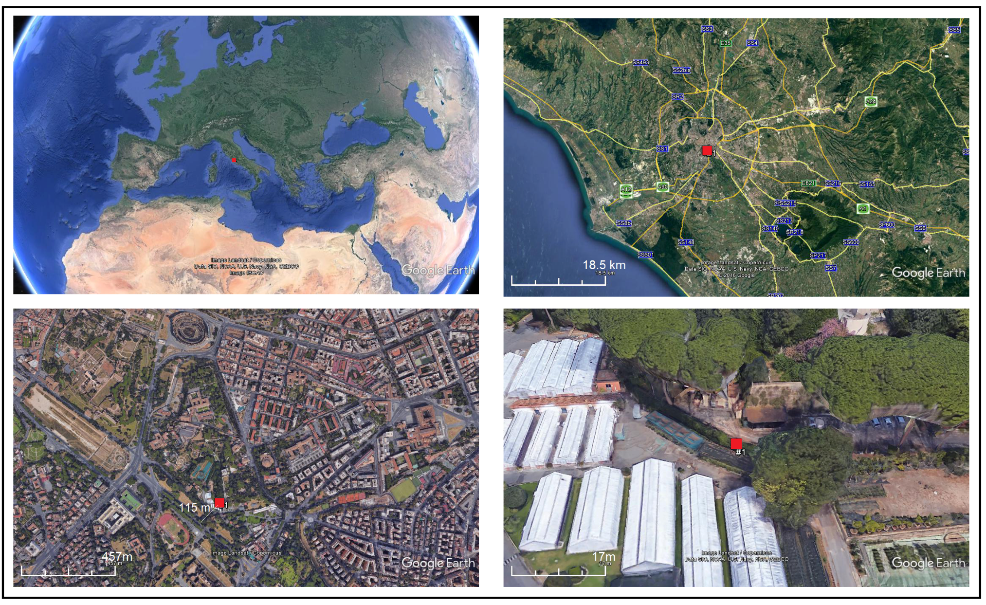
First, Table 7 points out that the levels of eBC and EC mass concentration are similar at the CARE site and at two other urban background sites in Rome: these data were measured (with similar instrumentation) during three different field campaigns in different years (2005, 2013, 2017 CARE, [74,75]). The fact that similar values occur at similar locations (but not in the immediate vicinity) in different years (and different months of the year) allows us to extend the results obtained, and to conclude that these values are representative of the urban background in Rome. The fact that the eBC at the CARE site (a park, more than 100 m away from the nearest traffic source, Figure 1) was not dominated by a single source is also supported by Figure 3b showing no influence from a single wind direction to the eBC mass concentration. Also, this is indicated by the MAC${}_{BC}$ values measured in the CARE experiment (8.6 ± 0.9 m${}^2$· g${}^{-1}$ at 637 nm), which are larger than values expected for freshly generated BC particles (at 550 nm, 7.5 ± 1.2 m${}^2$· g${}^{-1}$ [12], and thus less at 637 nm). The values reported at suburban background locations in Rome [74,76] are lower than values reported at these urban background sites (CARE, [74,75]). Combining all these data in Rome (Table 2, Table 3 and Table 7), we draw here the baseline levels for eBC and EC in the urban area of Rome:

• the mean value at suburban background sites of eBC mass concentration = about 1 $\mathsf{\mu }$g · m${}^{-3}$ ([76]);
• the mean value at urban background sites of eBC mass concentration in winter = 2.3–2.8 $\mathsf{\mu }$g · m${}^{-3}$, and EC mass concentration = 1.9–2.3 $\mathsf{\mu }$g · m${}^{-3}$ ([74,75,76] and Table 2);
• the mean daily maximum (1-min) concentration of eBC at urban background sites during winter = 5–5.5 $\mathsf{\mu }$g · m${}^{-3}$ (Table 3).

Second, Table 7 compares these eBC and EC mass concentration values in the urban background of Rome to values reported in literature at other urban background locations in Italy and Europe (London, Paris, Barcelona, Lugano). The (nineteen) sites in Italy were all classified as urban background sites, and include eight locations in the Po Valley, and one in Rome [74]. The site in Barcelona was characterized by a very dense road traffic network, one of the city’s main traffic avenues being located approximately 300 m from the site; the Lugano site was in a park in the city center, about 50 m to the east of a busy urban road; the London site was in North Kensington in the grounds of a school in a residential area [77]. The site in Paris was an AIRPARIF air quality monitoring network site representative of Paris background air pollution [78]. The values of eBC mass concentration reported at these urban background sites in Paris, Barcelona, London, and Lugano [77,78] are lower than the values reported at urban background sites in Rome (CARE, [75]). The mean EC mass concentration values reported in winter at urban background sites in Italy [74] are mostly lower (with a few exceptions at Po Valley sites) than values reported at urban background sites in Rome (CARE, [74]). The monthly average EC in February at different urban background sites in Barcelona calculated from 1999 to 2011 [23] is lower than the values reported at urban background sites in Rome (CARE, [74]). Note that the N${}_{tot}$ was lower in the CARE campaign than in the earlier studies (N${}_{tot}$ was lower only at a regional EMEP site [79]). This will be analysed in the future. There can be many possible explanations, and some of them may be partly derived from the instrumentation and measurement standards [80]: the SMPS was used in CARE, the CPC or WCPC in the earlier studies; measurement were carried out at RH < 30% in CARE (EUSAAR/ACTRIS protocol), and under ambient conditions in the earlier studies.

Finally, Table 7 also compares values of eBC mass concentration measured at different urban background sites during the case-study periods reported in Table 3: the rush hour of the working days, and the weekends at midday. The value in Rome is larger than values reported in Paris, London, Lugano and Barcelona [77,78]. This issue is discussed further in Section 4.2 and Section 4.3, and will be analysed in detail in the future.

4.2. On the Differences between Values at Urban Background and Traffic Sites

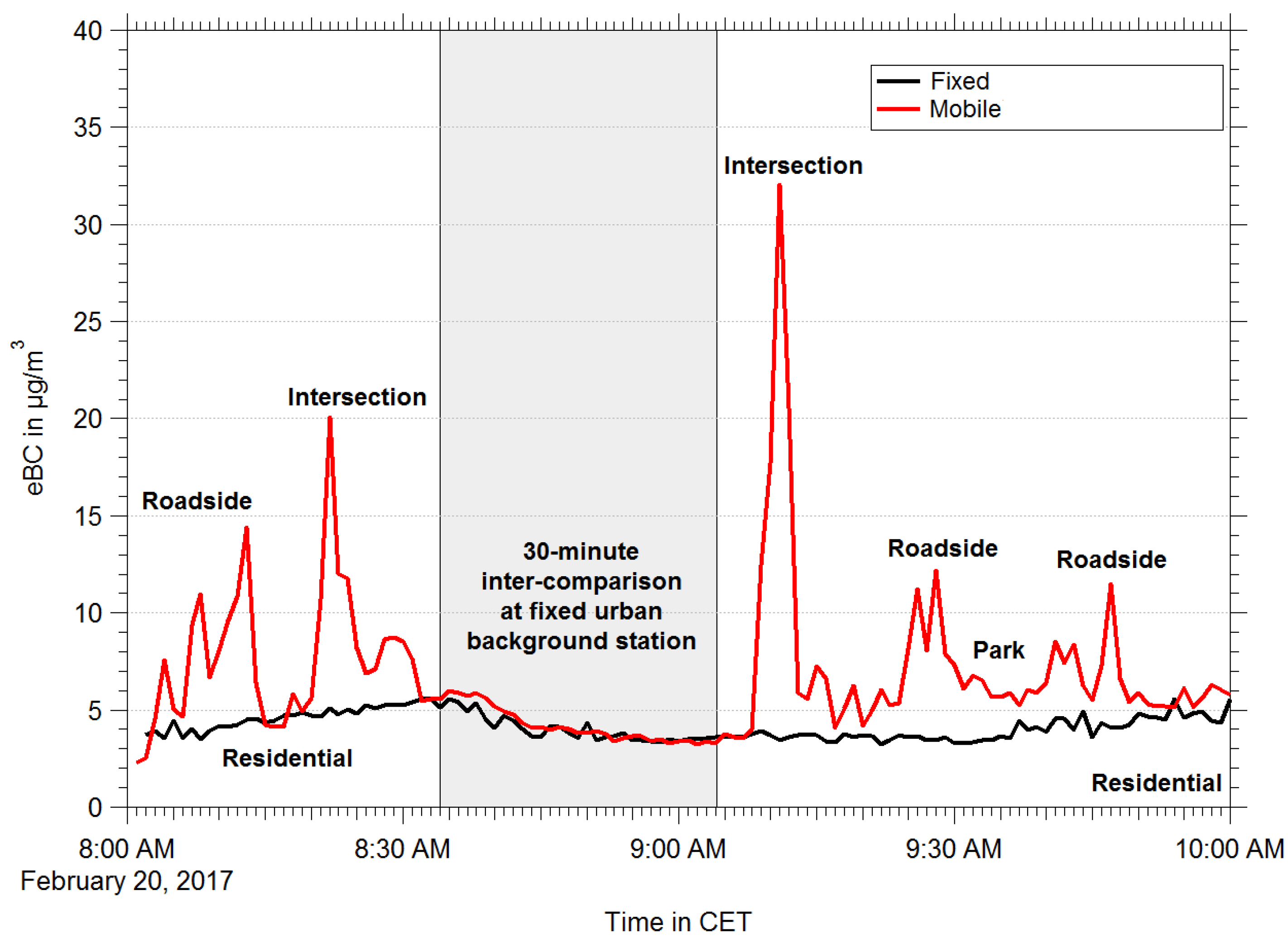
The aim of this section is to address differences between values measured at urban background and traffic sites in Rome. During the CARE experiment, additional eBC measurements were carried out while moving from emissions sources (e.g., roads) to parks to residential areas (cf. methodology, Section 2.3.15). The mobile measurement approach has the ability to capture the spatial variability or heterogeneity of eBC mass concentrations, which is a limitation of fixed stations. Mobile measurements during CARE will be the subject of a future paper. Here we show an example (Figure 10) of eBC mass concentrations measured during the morning rush hour (8:00–10:00 CET, 20 February 2017) at the CARE fixed station (black line) in comparison to that measured by mobile measurements (red line).

Concentrations measured at intersections with high vehicular traffic, traffic light areas, and along roads with street canyon configuration are significantly higher than those measured at the fixed station. Aside from vehicular emissions, high concentrations of eBC were also found along streets with restaurants using open fire heater for outdoor dining. This was more evident during the evening runs, characterised by lower temperatures and a larger number of open restaurants. Concentrations were found to decrease rapidly to urban background levels when entering traffic-limited regions such as residential, private, and park areas. Lower levels of eBC were also found along roads around tourist sites that are under traffic-limiting regulations.

Similar results were found in every single run performed throughout the campaign—details will be presented in a future publication. This shows that eBC concentrations measured closer to urban emission sources (e.g., at traffic lights) in Rome are much higher than those at the CARE urban background site. Note that peak values during this example (up to 30 $\mathsf{\mu }$g · m${}^{-3}$) are two times higher than the highest reported at the urban background site (up to 15 $\mathsf{\mu }$g · m${}^{-3}$, Figure 2a).

4.3. On the Data Averaging Period for the Carbonaceous Aerosol

The aim of this section is to discuss the data averaging period to be used for the carbonaceous aerosol in urban areas. The shorter term EU air quality limit value for PM${}_{10}$ rely on 24-h averaged data, meaning that all peak values occurring during the 24-h averaging period are considered as equally contributing to the average value. Here we intend to show how different these peak values are (in terms of particle composition, size distribution, and color), and question the appropriateness of using 24-h average for the carbonaceous aerosol.

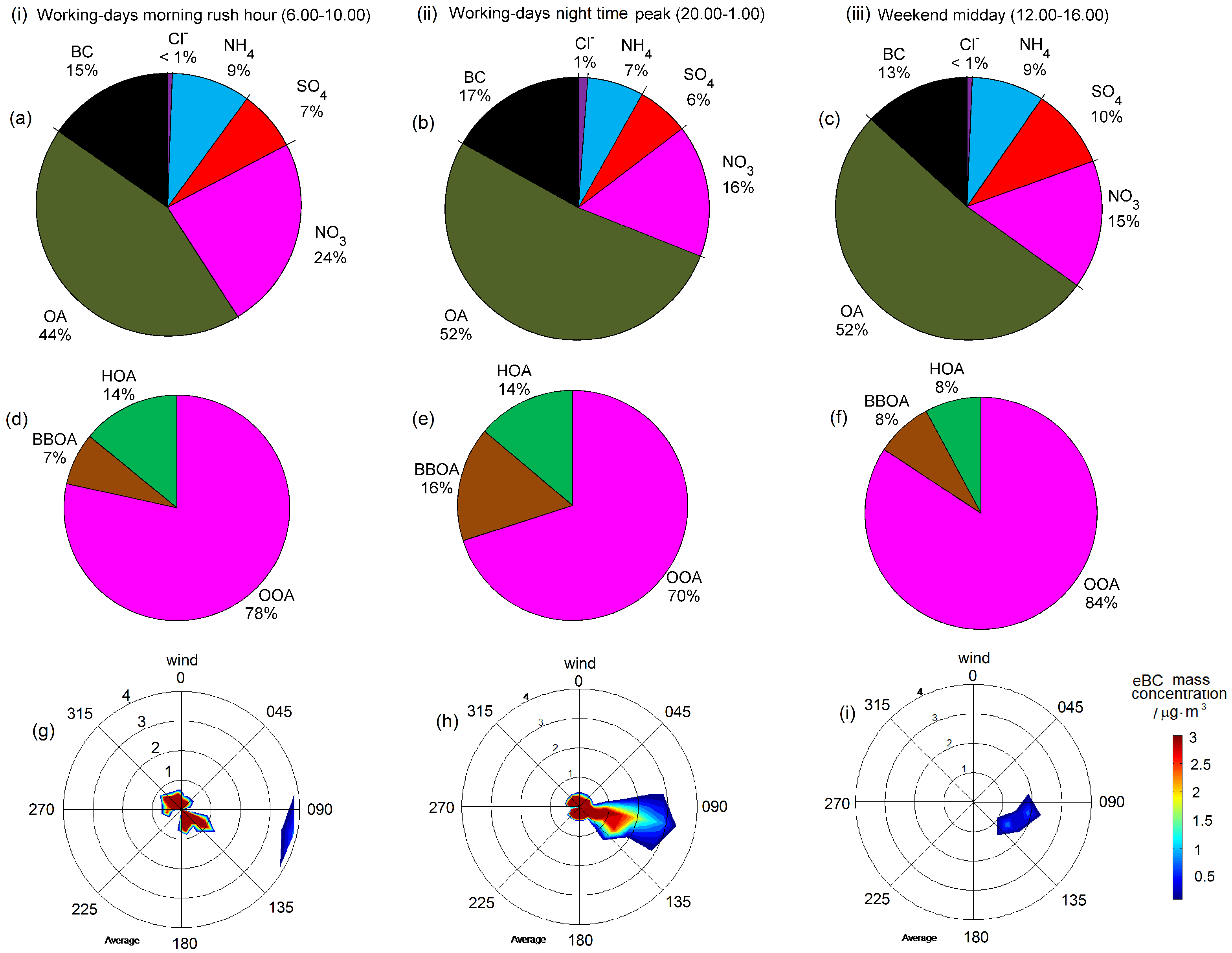
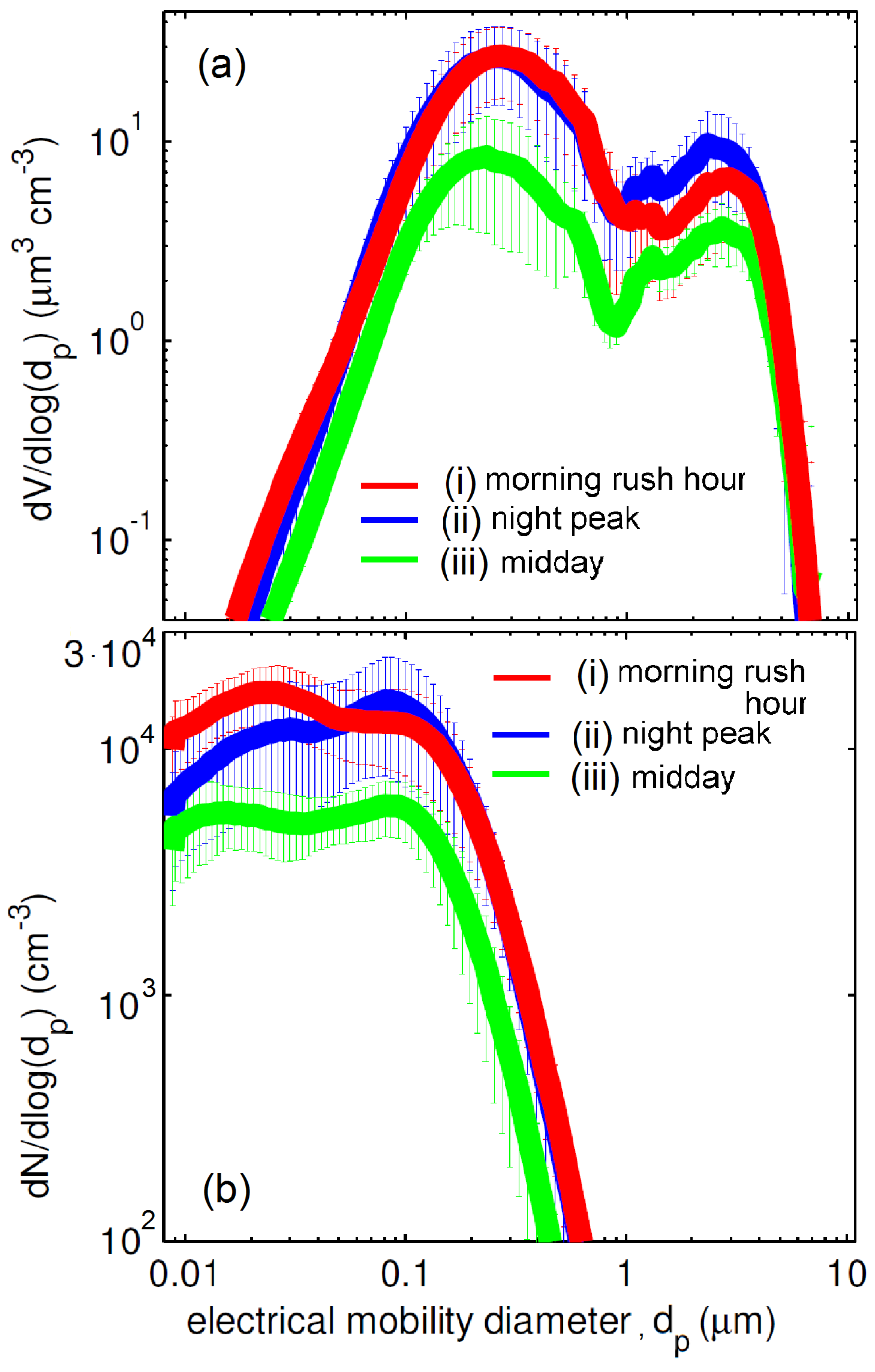
We analyse and compare three different cases: (i) the week-day morning rush hour (6.00–10.00, LT); (ii) the week-day night peak (20.00–00.59, LT); and (iii) the weekend midday (12.00–16.00, LT). This is explored in Figure 11, Figure 12 and Figure 13 and Table 3 showing:

• major components of PM${}_1$ (panels a, b, c of Figure 11),
• contributions to the total OA in NR-PM${}_1$ of the major emission sources identified (Vehicular traffic emission (HOA), Biomass burning emission (BBOA), and Oxygenated secondary aerosol (OOA)) (panels d, e , f of Figure 11);
• wind conditions (panels g, h, i of Figure 11);
• particle size distributions (Figure 12);
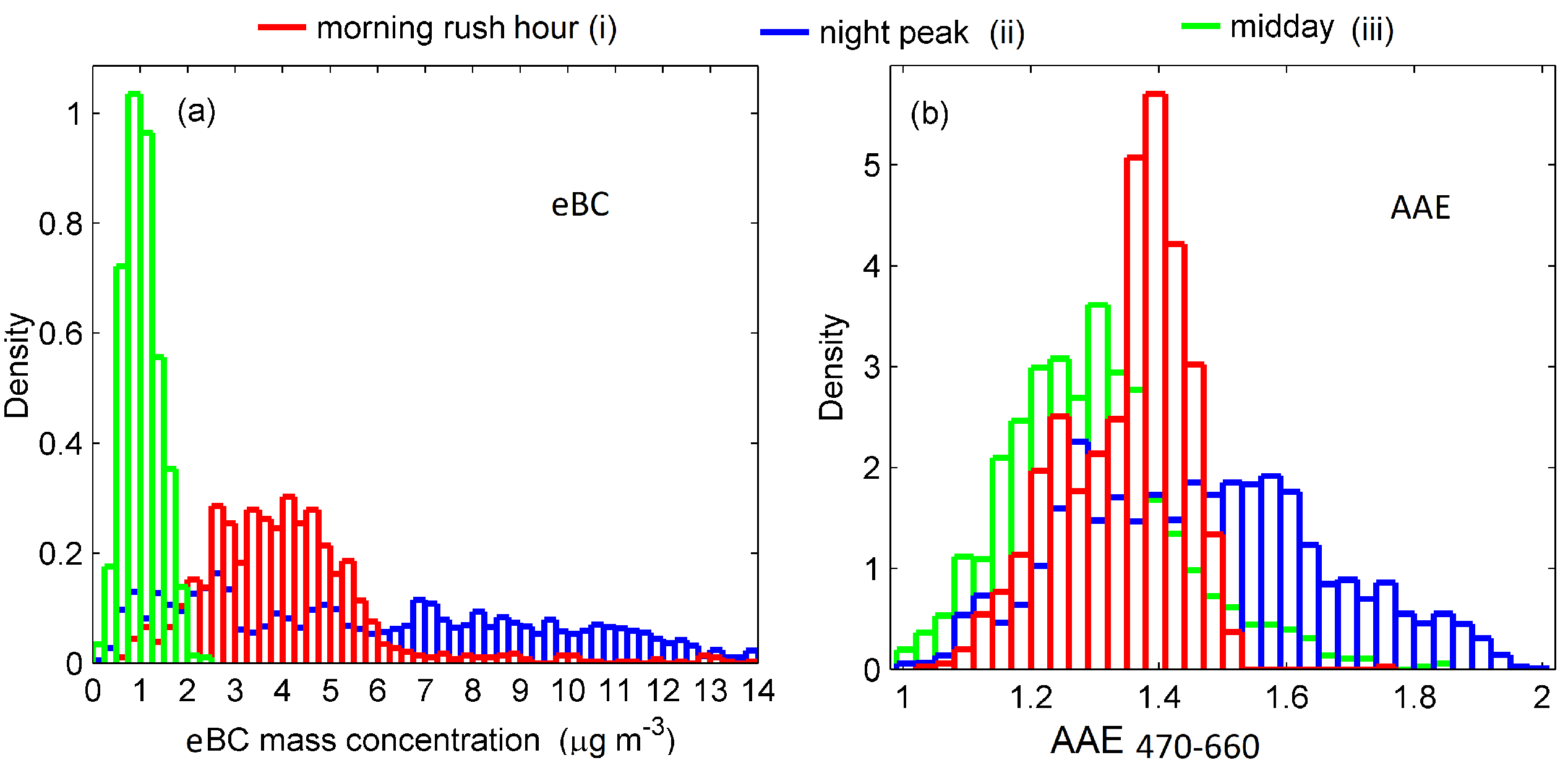
• eBC and AAE (as probability density functions, pdf, Figure 13);
• all descriptive statistics (Table 3).

At the morning rush hour (case (i)) we observe:

• HOA contribution larger than BBOA contribution (unlike case (ii), Figure 11d,e),
• the largest NO${}_3^{-}$ contribution to PM${}_1$ (Figure 11a),
• the highest UFP number concentration and N${}_{tot}$ (Figure 4d),
• the largest BC-to-PM${}_1$ and EC-to-OC (Figure 4f),
• the lowest SSA (Figure 4i),
• higher concentration of aged nucleation mode particles (diameter of 20–30 nm in Figure 12b) than for case (ii).

In this case (i), we likely measured the (shortly aged) road traffic related aerosol. Unlike case (i), at the night peak hour (case (ii)) we observe:

• equal contributions of biomass burning and road traffic emissions ( Figure 11d,e),
• bimodality of the AAE pdf and large variability of eBC values (Figure 13),
• higher OA contribution to PM1 than in case (i), despite the fact that the BC to OA ratio is similar in both cases (eBC-to-OA of 0.33–0.34),
• the largest mean eBC mass concentrations (Table 3),
• eBC contribution to PM${}_1$ larger than that of NO${}_3^{-}$ ( Figure 11),
• larger aerosol size than in case (i) (Figure 4e),
• higher concentration of soot particles (diameter of 80–100 nm in Figure 12b, explaining the larger eBC mass concentration) and coarse mode particles (diameter > 1 $\mathsf{\mu }$m in Figure 12a) than for case (i).

In this case (ii), the aerosol is probably a combination of different sources differently aged in the atmosphere. At midday case (iii) the aerosol had mass and number concentrations much lower (more than four times lower), and a higher OOA contributions. This case is intended to contrast conditions represented in the cases already described cases (i) and (ii).

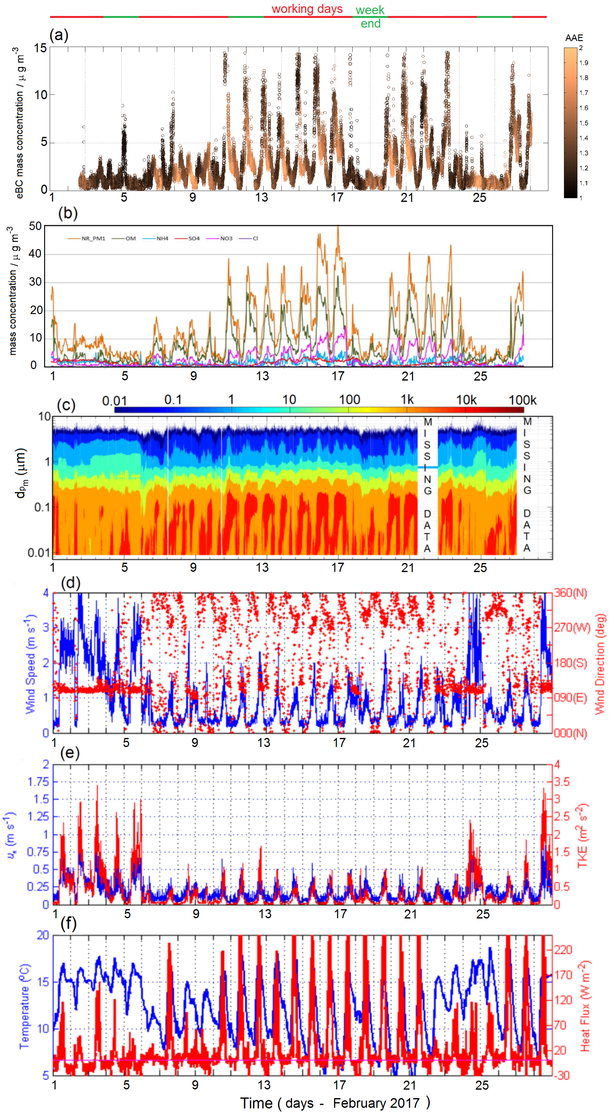
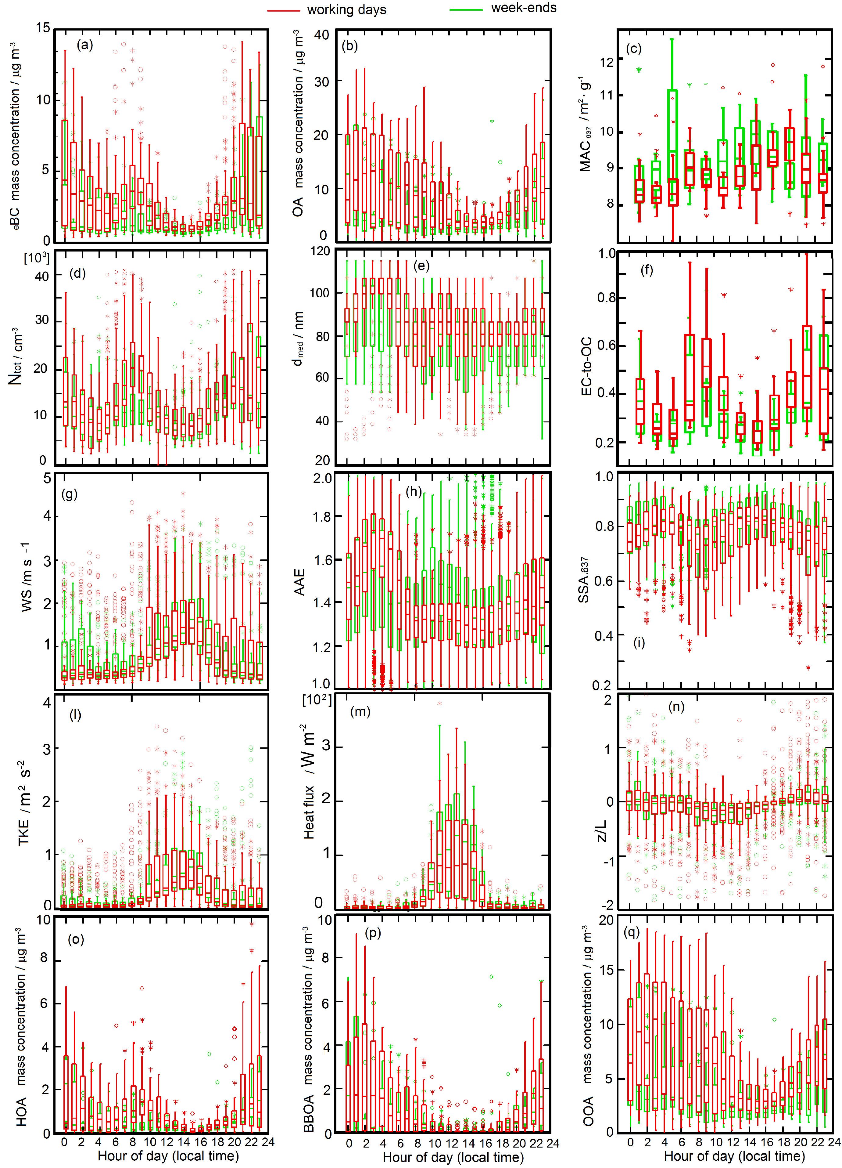
Note that the three cases selected (morning rush hour, night peak hour, and midday) are commonly characterized by different atmospheric conditions. This includes different boundary layer dynamics, which also likely play a role in influencing aerosol total concentration. The best dispersion of atmospheric pollutants is observed during the central hours of the day case (iii), with a maximum from 02:00 to 16:00 (cf. diurnal cycles in Figure 4 and Figure S23 of the supplementary Materials). During the afternoon, a progressive stabilization of the atmosphere is observed, which lasts until the late morning of the following day, with a maximum at sunrise. This is reflected in the relationship between mass concentration and wind (panels g–i of Figure 11) for reasons of space, we show eBC only. The larger eBC mass concentrations at the morning rush hour case (i) are caused by the combination of low dispersion, low winds (<1 m·s${}^{-1}$, Figure 11g) and increased local aerosol emissions (mainly from road traffic, according to Figure 11d). The (very) high eBC concentration at the night peak hour case (ii) have various causes: biomass burning emissions were larger than during the morning hours case (i); wind speeds were often as low as on the case (i) (Figure 11). The latter situation highlights the role of emissions: by comparing panel h and i of Figure 11, we observe that the eBC concentration is larger at the night peak hour than at midday, despite the same wind conditions (wind speed of 1 to 2 m·s${}^{-1}$ from E-SE). Finally, it is worth noting that the eBC mass concentration at the CARE site is not dominated by a single source (Figure 3b), and that there is no influence from a single wind direction even during the selected case-studies (e.g., the morning rush hour in Figure 11g).

These findings point to the importance of considering proper time-scales to analyse carbonaceous aerosol properties. These are clearly shorter than 24 h, and the use of a 24-h data averaging period can significantly limit findings. Based on these findings, in Section 4.4 we will analyse relevant toxicological data with the aim to provide recommendations for acute exposure studies.

4.4. Toxicological Implications

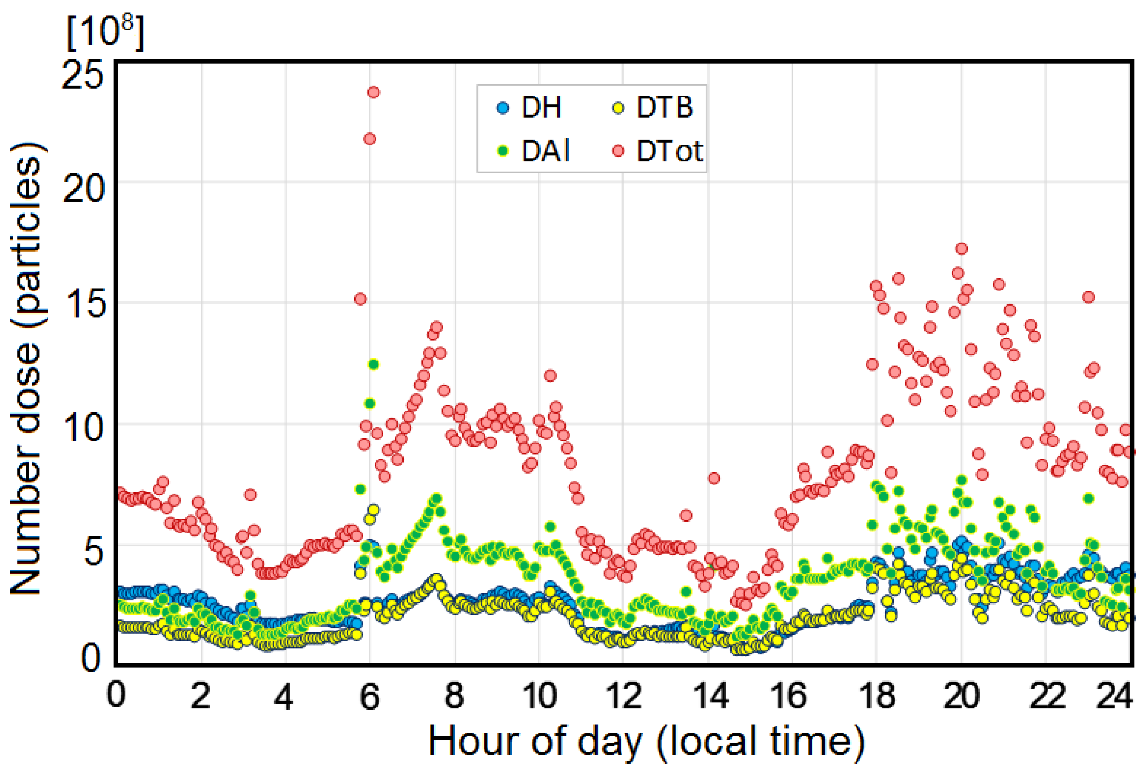
In this paper we presented for the first time to our knowledge the use of an ALI exposure system for the direct exposure of an in vitro system to airborne particulate matter under real environmental conditions. Preliminary results indicate no clear sign of cytotoxicity in cells exposed for 24 h (Section 3.3.2). The regulation of genes involved in cellular pathways of interest will be evaluated in future. Future analysis will include the assessment of the aerosol number dose deposited in the human body (Section 3.3.3). Here we reported (Figure 9) the aerosol number doses deposited in the head (H), tracheobronchial (TB) and alveolar (Al) regions along with the relevant total dose estimated (we show 20 February 2017, the same day as for eBC mass concentrations measurements in Figure 10). These preliminary results indicate that number doses and deposition in different regions of the body change with time during the 24 h (e.g., rush hour vs. midday vs. night).

Future analysis will couple these data and the aerosol data, to the oxidative potential data presented in Section 3.3 and biomonitoring data presented in Section 3.3.4. The aim will be to link carbonaceous aerosol levels in the atmosphere to the real human exposure. Preliminary findings suggest that human exposure to carbonaceous aerosol can be correlated to eBC mass concentrations [73]. The premise for this exercise will be the increasing awareness that carbonaceous aerosols may induce health effects through the generation of oxidative stress [15,81,82,83,84]. 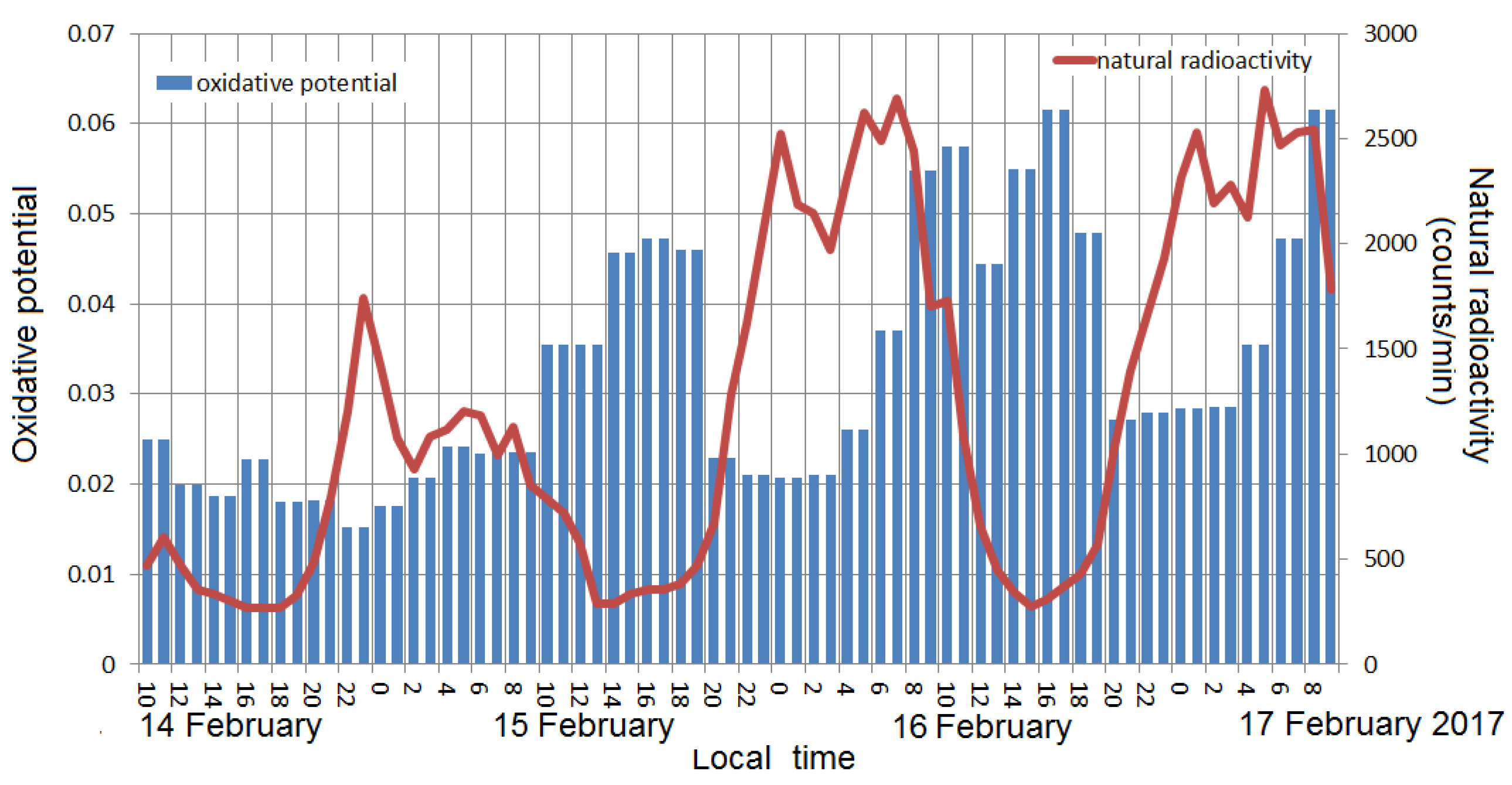The biomonitoring data will provide information on the oxidative stress (Section 3.3.4), defined as an imbalance between the level of reactive oxygen species (ROS, or free radicals) and the natural antioxidant defence of the biological system. It is commonly thought that ROS can damage lipids, proteins, and membrane DNA, and can also cause cell death by necrotic or apoptotic processes. The oxidative potential (OP) associated with aerosol particles (Section 3.3.1) is considered as a proxy of the ability of PM${}_x$ to generate ROS, and is defined as the capacity of PM${}_x$ to oxidize target molecules. The measurement of the OP was proposed as a possible air quality exposure metric. The relation between the oxidative stress and the OP will be analysed in future studies. Here, we present a preliminary analysis of the OP data.

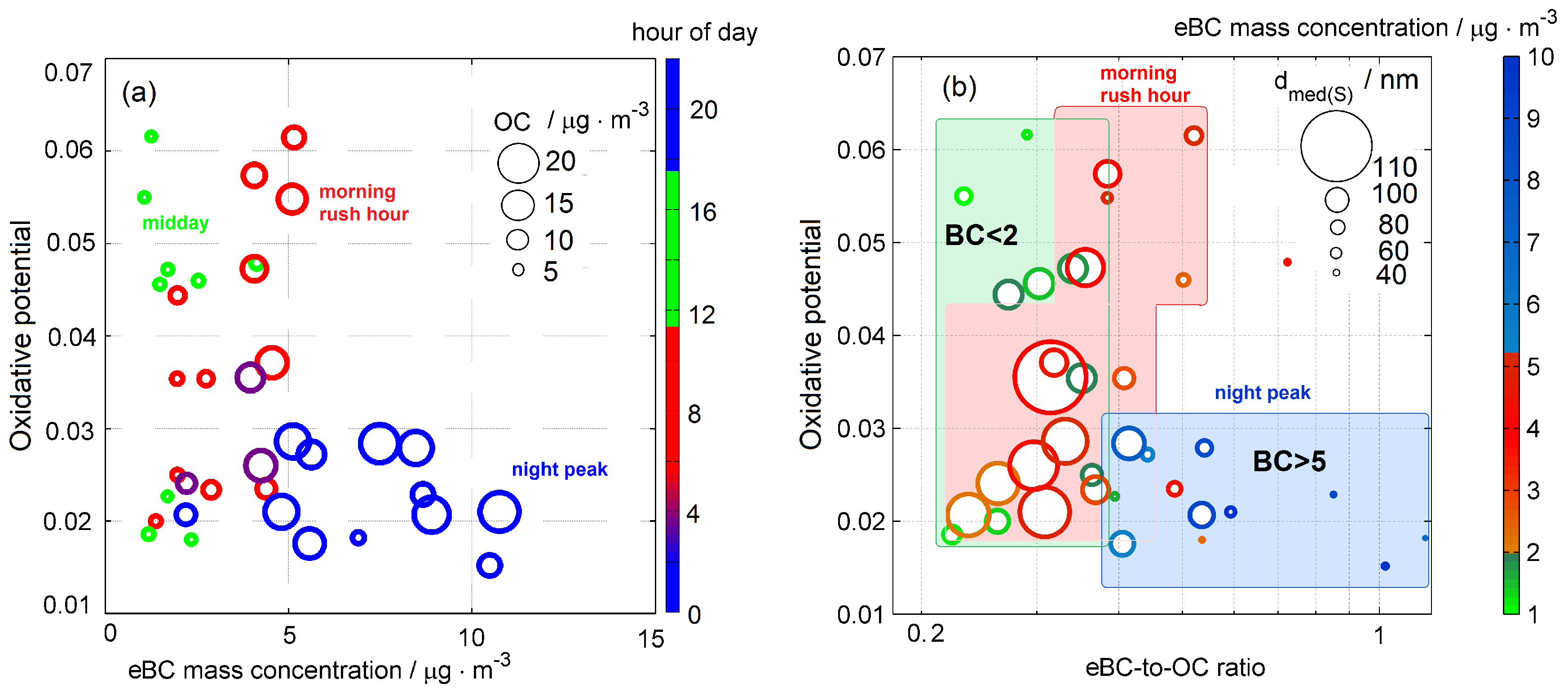
Figure 14 shows the OP data presented in Figure 8 separately during the three different scenarios identified in Section 4.3, i.e., morning rush hour, night peak and midday (Figure 11, Figure 12 and Figure 13 and Table 3 note that red, blue and green markers in Figure 14 show these three cases, respectively).

Considering Figure 14a, the aerosol occurring at the night peak hour (blue markers) correspond to the lowest values of the oxidative potential and to the highest eBC mass concentration. Conversely, the aerosol occurring at the morning rush hour (red markers) might have significantly larger values of the OP if associated with smaller particle size. Indeed, at the morning rush hour we observed a particle size-dependent OP: the OP tends to increase with decreasing aerosol median diameter (Figure 14b).

These preliminary findings reinforce existing concerns about the toxicity of carbonaceous aerosols [2,3,4,7,8,11]. We support literature findings indicating that the toxicological risk of carbonaceous aerosol might depend on both particle size and composition (e.g., BC levels). Also, we show that BC toxicity may increase with decreasing particle size, but only for certain conditions—i.e., the morning rush hour case-study, during our experiment. The same does not apply to the night peak case-study, which shows the highest values of the BC mass concentration with small particle size, but has the lowest toxicological effects. Future studies will look into possible causes for these differences, including certain combinations of particle size and chemical composition. Also, a comparative campaign in a contrasting season such as late summer is likely to be carried out.

5. Conclusions

In February 2017, the “Carbonaceous Aerosol in Rome and Environs (CARE)” experiment was carried out to address the following specific questions: what is the color, size, composition, and toxicity of the carbonaceous aerosol in the urban background area of the city of Rome? The motivation of this experiment is the lack of understanding of what aerosol types are responsible for the severe risks to the human health posed by particulate matter (PM) pollution, as well as how carbonaceous aerosols influence radiative balance. To answer these questions, physicochemical properties and toxicity of the carbonaceous aerosol were characterised in the downtown Rome with high time resolution (minutes to hours).

Preliminary findings of the CARE experiment presented in this paper:

• Baseline levels for urban background aerosols in Rome were determined, with mean eBC mass concentration in winter of 2.6 ± 2.5 $\mathsf{\mu }$g · m${}^{-3}$ and mean eBC peak value of 5.2 (95% CI = 5.0–5.5) $\mathsf{\mu }$g · m${}^{-3}$ (mean of the daily maximum 1-min average concentration);
• Mean values of eBC and EC mass concentration in Rome were found to be larger than values observed across other European cities, especially during the peak values (typically lasting less than 1 h);
• The effects of toxicity associated with the carbonaceous aerosol were found to be higher for smaller particle sizes that typically occur at low mass concentrations.

These findings:

• reinforce existing concerns about the toxicity of carbonaceous aerosols,
• support the existing evidence indicating that particle size distribution and composition may play a role in the generation of this toxicity,
• reinforce the need to consider an averaging period shorter or equal to 1 h to address carbonaceous aerosol toxicity.

We believe that the existing air quality standards for PM${}_{10}$ and PM${}_{2.5}$ in Europe have to be complemented with new standards to address carbonaceous aerosol toxicity. We suggest that these new standards are based on ultrafine particles and/or BC/EC measurements with better time resolution than 24 h mean concentrations (which is used by air quality standards for PM${}_{10}$).

Preliminary CARE findings point to the following significant limitations in these current standards:

• since there is only one standard for particulate matter, namely PM${}_{10}$ (i.e., the total mass of all particles smaller than 10 $\mathsf{\mu }$m), all particles smaller than 10 $\mathsf{\mu }$m are often treated as equally toxic, with no regard for particle composition and size;
• the consideration of mass only (no number and no size metric) neglects the role of the smaller particles (i.e., UFPs) dominating the black, elemental carbon and fresh/primary organic aerosol particles from combustion sources (UFPs are typically characterised by lower mass and larger number concentrations);
• the consideration of data averaging periods of 24 h (or one year) considers all peak values (typically lasting less than 1 h) as equally contributing to the average value.

We recommend that these air quality standards are updated by including measurements of particle composition (at least BC) and particle number (and size) with shorter data averaging period (less than 1 h). Indeed, for understanding health effects these parameters have to be addressed. More research is however still needed to investigate in detail how this can be done in a scientifically sound and consistent way that is useful for improving the environment and health.

References

1. Shindell, D.; Kuylenstierna, J.C.; Vignati, E.; van Dingenen, R.; Amann, M.; Klimont, Z.; Schwartz, J. Simultaneously mitigating near-term climate change and improving human health and food security. Science 2012, 335, 183–189. [Google Scholar] [CrossRef] [PubMed]
2. Lelieveld, J.; Evans, J.S.; Fnais, M.; Giannadaki, D.; Pozzer, A. The contribution of outdoor air pollution sources to premature mortality on a global scale. Nature 2015, 525, 367–371. [Google Scholar] [CrossRef] [PubMed]
3. Janssen, N.A.H.; Gerlofs-Nijland, M.E.; Lanki, T.; Salonen, R.O.; Cassee, F.; Hoek, G.; Fischer, P.; Brunekreef, B.; Krzyzanowski, M. Health Effects of Black Carbon; World Health Organization, Regional Office for Europe: Copenhagen, Denmark, 2012. [Google Scholar]
4. World Health Organization. Review of Evidence on Health Aspects of Air Pollution REVIHAAP Project; Technical Report; World Health Organization: Copenhagen, Denmark, 2013. [Google Scholar]
5. Lim, S.S.; Vos, T.; Flaxman, A.D.; Danaei, G.; Shibuya, K.; Adair-Rohani, H.; AlMazroa, M.A.; Amann, M.; Anderson, H.R.; Andrews, K.G.; et al. A comparative risk assessment of burden of disease and injury attributable to 67 risk factors and risk factor clusters in 21 regions, 1990–2010: A systematic analysis for the Global Burden of Disease Study 2010. Lancet 2012, 380, 2224–2260. [Google Scholar] [CrossRef]
6. US EPA. Integrated Science Assessment for Particulate Matter (Final Report); Agency USEP: Washington, DC, USA, 2009.
7. Cassee, F.R.; Heroux, M.E.; Gerlofs-Nijland, M.E.; Kelly, F.J. Particulate matter beyond mass: Recent health evidence on the role of fractions, chemical constituents and sources of emission. Inhal. Toxicol. 2013, 25, 802–812. [Google Scholar] [CrossRef] [PubMed]
8. UNEP WMO (United Nations Environment Programme and World Meteorological Organization). Integrated Assessment of Black Carbon and Tropospheric Ozone; UNEP WMO (United Nations Environment Programme and World Meteorological Organization): Nairobi, Kenya, 2011; p. 285. [Google Scholar]
9. US National Academy of Sciences; Committee on Research Priorities for Airborne Particulate Matter NRC. Research Priorities for Airborne Particulate Matter: IV. Continuing Research Progress; The National Academies Press: Washington, DC, USA, 2004. [Google Scholar]
10. HEI. Understanding the Health Effects of Components of the Particulate Matter Mix: Progress and Next Steps; Technical Report 4; Health Effects Institute: Boston, MA, USA, April 2002. [Google Scholar]
11. Tuomisto, J.T.; Wilson, A.; Evans, J.S.; Tainio, M. Uncertainty inmortality response to airborne fine particulate matter: Combining European air pollution experts. Reliab. Eng. Syst. Saf. 2008, 93, 732–744. [Google Scholar] [CrossRef]
12. Bond, T.C.; Doherty, S.J.; Fahey, D.W.; Forster, P.M.; Berntsen, T.; DeAngelo, B.J.; Flanner, M.G.; Ghan, S.; Kärcher, B.; Koch, D.; et al. Bounding the role of black carbon in the climate system: A scientific assessment. J. Geophys. Res. Atmos. 2013, 118, 5380–5552. [Google Scholar] [CrossRef] [Green Version]
13. Oberdörster, G.; Oberdörster, E.; Oberdörster, J. Nanotoxicology: An Emerging Discipline Evolving from Studies of Ultrafine Particles. Environ. Health Perspect. 2005, 113, 823–839. [Google Scholar] [CrossRef] [PubMed]
14. Block, M.L.; Calderon-Garciduenas, L. Air pollution: Mechanisms of neuroinflammation and CNS disease. Trends Neurosci. 2009, 32, 506–516. [Google Scholar] [CrossRef] [PubMed]
15. Li, N.; Sioutas, C.; Cho, A.; Schmitz, D.; Misra, C.; Sempf, J.; Wang, M.; Oberley, T.; Froines, J.; Nel, A. Ultrafine particulate pollutants induce oxidative stress and mitochondrial damage. Environ. Health Perspect. 2003, 111, 455–460. [Google Scholar] [CrossRef] [PubMed]
16. Stafoggia, M.; Schneider, A.; Cyrys, J.; Samoli, E.; Andersen, J.; Bero Bedada, Z.G.; Bellander, T.; Cattani, G.; Eleftheriadis, K.; Faustini, A.; et al. Association Between Short-term Exposure to Ultrafine Particles and Mortality in Eight European Urban Areas. Epidemiology 2017, 28, 172–180. [Google Scholar] [CrossRef] [PubMed]
17. Myhre, G.; Samset, B.H.; Schulz, M.; Balkanski, Y.; Bauer, S.; Berntsen, T.K.; Bian, H.; Bellouin, N.; Chin, M.; Diehl, T.; et al. Radiative forcing of the direct aerosol effect from AeroCom Phase II simulations. Atmos. Chem. Phys. 2013, 13, 1853–1877. [Google Scholar] [CrossRef]
18. Baumgardner, D.; Popovicheva, O.; Allan, J.; Bernardoni, V.; Cao, J.; Cavalli, F.; Cozic, J.; Diapouli, E.; Eleftheriadis, K.; Genberg, P.J.; et al. Soot reference materials for instrument calibration and intercomparisons: A workshop summary with recommendations. Atmos. Meas. Tech. 2012, 5, 1869–1887. [Google Scholar] [CrossRef] [Green Version]
19. DeCarlo, P.F.; Kimmel, J.R.; Trimborn, A.; Northway, M.J.; Jayne, J.T.; Aiken, A.C.; Gonin, M.; Fuhrer, K.; Horvath, T.; Docherty, K.S.; et al. Field-deployable, high-resolution, time-of-flight aerosol mass spectrometer. Anal. Chem. 2006, 78, 8281–8289. [Google Scholar] [CrossRef] [PubMed]
20. Kulmala, M.; Asmi, A.; Lappalainen, H.K.; Baltensperger, U.; Brenguier, J.L.; Facchini, M.C.; Hansson, H.-C.; O’Dowd, C.D.; Pöschl, U.; Boers, R.; et al. General overview: European Integrated project on Aerosol Cloud Climate and Air Quality interactions (EUCAARI)–integrating aerosol research from nano to global scales. Atmos. Chem. Phys. 2011, 11, 13061–13143. [Google Scholar] [CrossRef] [Green Version]
21. Alves, C.; Vicente, A.; Pio, C.; Kiss, G.; Hoffer, A.; Decesari, S.; Prevot, A.S.H.; Minguillon, M.C.; Querol, X.; Hillamo, R.; et al. Organic compounds in aerosols from selected European sites e Biogenic versus anthropogenic sources. Atmos. Environ. 2012, 59, 243–255. [Google Scholar] [CrossRef]
22. Cavalli, F.; Alastuey, A.; Areskoug, H.; Ceburnis, D.; Genberg, J.; Harrison, R.M.; Jaffrezo, J.L.; Kiss, G.; Aas, W.; Putaud, J.P.; et al. A European aerosol phenomenology -4: Harmonized concentrations of carbonaceous aerosol at 10 regional background sites across Europe. Atmos. Environ. 2016, 144, 133–145. [Google Scholar] [CrossRef]
23. Querol, X.; Alastuey, A.; Viana, M.; Moreno, T.; Reche, C.; Minguillón, M.C.; Ripoll, A.; Pandolfi, M.; Amato, F.; Karanasiou, A.; et al. Variability of carbonaceous aerosols in remote, rural, urban and industrial environments in Spain: Implications for air quality policy. Variability of carbonaceous aerosols in remote, rural, urban and industrial environments in Spain: Implications for air quality policy. Atmos. Chem. Phys. 2013, 13, 6185–6206. [Google Scholar]
24. Lelieveld, J.; Berresheim, H.; Borrmann, S.; Crutzen, P.J.; Dentener, F.J.; Fischer, H.; Korrmann, R. Global air pollution crossroads over the Mediterranean. Science 2002, 298, 794–799. [Google Scholar] [CrossRef] [PubMed]
25. Drinovec, L.; Močnik, G.; Zotter, P.; Prévôt, A.S.H.; Ruckstuhl, C.; Coz, E.; Rupakheti, M.; Sciare, J.; Müller, T.; Wiedensohler, A.; et al. The “dual-spot” Aethalometer: An improved measurement of aerosol black carbon with real-time loading compensation. Atmos. Meas. Tech. 2015, 8, 1965–1979. [Google Scholar] [CrossRef]
26. Müller, T.; Henzing, J.S.; de Leeuw, G.; Wiedensohler, A.; Alastuey, A.; Angelov, H.; Bizjak, M.; Collaud Coen, M.; Engström, J.E.; Gruening, C.; et al. Characterization and intercomparison of aerosol absorption photometers: Result of two intercomparison workshops. Atmos. Measurem. Techn. 2011, 4, 245–268. [Google Scholar] [CrossRef] [Green Version]
27. Vecchi, R.; Bernardoni, V.; Paganelli, C.; Valli, G. A filter-based light-absorption measurement with polar photometer: Effects of sampling artefacts from organic carbon. J. Aerosol Sci. 2014, 70, 15–25. [Google Scholar] [CrossRef]
28. Bernardoni, V.; Valli, G.; Vecchi, R. Set-up of a multi wavelength polar photometer for off-line absorption coefficient measurements on 1-h resolved aerosol samples. J. Aerosol Sci. 2017, 107, 84–93. [Google Scholar] [CrossRef]
29. Petzold, A.; Schölinner, M. Multi-angle absorption photometry—A new method for the measurement of aerosol light absorption and atmospheric black carbon. J. Aerosol Sci. 2004, 35, 421–441. [Google Scholar] [CrossRef]
30. Giannoni, M.; Calzolai, G.; Chiari, M.; Cincinelli, A.; Lucarelli, F.; Martellini, T.; Nava, S. A comparison between thermal-optical transmittance elemental carbon measured by different protocols in PM2.5 samples. Sci. Total Environ. 2016, 571, 195–205. [Google Scholar] [CrossRef] [PubMed]
31. Sanna Saarikoski, S.; Sillanpa, M.; Sofiev, M.; Timonen, H.; Saarnio, K.; Teinila, K.; Karppinen, A.; Kukkonen, J.; Hillamo, R. Chemical composition of aerosols during a major biomass burning episode over northern Europe in spring 2006: Experimental and modelling assessments. Atmos. Environ. 2007, 41, 3577–3589. [Google Scholar] [CrossRef]
32. Lukacs, H.; Gelencser, A.; Hammer, S.; Puzbaum, H.; Pio, C.; Legrand, M.; Kasper-Giebl, A.; Handler, M.; Limbeck, A.; Simpson, D.; et al. Seasonal trends and possible sources of brown carbon based on 2-year aerosol measurements at six sites in Europe. J. Geophys. Res. 2007, 112, D23S18. [Google Scholar] [CrossRef]
33. Hecobian, A.; Zhang, X.; Zheng, M.; Frank, N.; Edgerton, E.S.; Weber, R.J. Water-Soluble Organic Aerosol material and the light-absorption characteristics of aqueous extracts measured over the Southeastern United States. Atmos. Chem. Phys. 2010, 10, 5965–5977. [Google Scholar] [CrossRef]
34. Calzolai, G.; Lucarelli, F.; Chiari, M.; Nava, S.; Giannoni, M.; Carraresi, L.; Prati, P.; Vecchi, R. Improvements in PIXE analysis of hourly particulate matter samples. Nucl. Instr. Meth. B 2015, 363, 99–104. [Google Scholar] [CrossRef]
35. Lucarelli, F.; Calzolai, G.; Chiari, M.; Giannoni, M.; Mochi, D.; Nava, S.; Carraresi, L. The upgraded external-beam PIXE/PIGE set-up at LABEC for very fast measurements on aerosol samples. Nucl. Instr. Meth. B 2014, 318, 55–59. [Google Scholar] [CrossRef]
36. Ng, N.L.; Herndon, S.C.; Trimborn, A.; Canagaratna, M.R.; Croteau, P.; Onasch, T.M.; Sueper, D.; Worsnop, D.R.; Zhang, Q.; Sun, Y.L.; et al. An Aerosol Chemical Speciation Monitor (ACSM) for routine monitoring of atmospheric aerosol composition. Aerosol Sci. Technol. 2011, 45, 770–784. [Google Scholar] [CrossRef]
37. Fröhlich, R.; Crenn, V.; Setyan, A.; Belis, C.A.; Canonaco, F.; Favez, O.; Riffault, V.; Slowik, J.G.; Aas, W.; Aijälä, M.; et al. ACTRIS ACSM intercomparison—Part 2: Intercomparison of ME-2 organic source apportionment results from 15 individual, co-located aerosol mass spectrometers. Atmos. Meas. Tech. 2015, 8, 2555–2576. [Google Scholar] [CrossRef] [Green Version]
38. Hinds, W.C. Aerosol Technology, 2nd ed.; Wiley: New York, NY, USA, 1999. [Google Scholar]
39. Khlystov, A.; Stanier, C.; Pandis, S.N. An algorithm for combining electrical mobility and aerodynamic size distributions data when measuring ambient aerosol special issue of aerosol science and technology on findings from the fine particulate matter supersites program. Aerosol Sci. Technol. 2004, 38, 229–238. [Google Scholar] [CrossRef]
40. Amato, F.; Pandolfi, M.; Moreno, T.; Furger, M.; Pey, J.; Alastuey, A.; Bukowiecki, N.; Prevot, A.S.H.; Baltensperger, U.; Querol, X. Sources and variability of inhalable road dust particles in three European cities. Atmos. Environ. 2011, 45, 6777–6787. [Google Scholar] [CrossRef]
41. Amato, F.; Schaap, M.; Denier van der Gon, H.A.C.; Pandolfi, M.; Alastuey, A.; Keuken, M.; Querol, X. Effect of rain events on the mobility of road dust load in two Dutch and Spanish roads. Atmos. Environ. 2012, 62, 352–358. [Google Scholar] [CrossRef]
42. Querol, X.; Alastuey, A.; Rodríguez, S.; Plana, F.; Mantilla, E.; Ruiz, C.R. Monitoring of PM10 and PM2.5 around primary particulate anthropogenic emission sources. Atmos. Environ. 2001, 35, 845–858. [Google Scholar] [CrossRef]
43. Cavalli, F.; Viana, M.; Yttri, K.E.; Genberg, J.; Putaud, J.-P. Toward a standardised thermal-optical protocol for measuring atmospheric organic and elemental carbon: The EUSAAR protocol. Atmos. Meas. Technol. 2010, 3, 79–89. [Google Scholar] [CrossRef] [Green Version]
44. China, S.; James, D.E. Influence of pavement macrotexture on PM10 emissions from paved roads: A controlled study. Atmos. Environ. 2012, 63, 313–326. [Google Scholar] [CrossRef]
45. Perrino, C.; Pietrodangelo, A.; Febo, A. An atmospheric stability index based on radon progeny measurements for the evaluation of primary urban pollution. Atmos. Environ. 2001, 35, 5235–5244. [Google Scholar] [CrossRef]
46. Perrino, C.; Canepari, S.; Catrambone, M.; Dalla Torre, S.; Rantica, E.; Sargolini, T. Influence of natural events on the concentration and composition of atmospheric particulate matter. Atmos. Environ. 2009, 43, 4766–4779. [Google Scholar] [CrossRef]
47. Perrino, C.; Catrambone, M.; Farao, C.; Salzano, R.; Esposito, G.; Giusto, M.; Montagnoli, M.; Marini, A.; Brinoni, M.; Simonetti, G.; et al. Improved Time-Resolved Measurements of Inorganic Ions in Particulate Matterby PILS-IC Integrated with a Sample Pre-Concentration System. Aerosol Sci. Technol. 2015, 49, 521–530. [Google Scholar] [CrossRef]
48. Aufderheide, M.; Scheffler, S.; Mohle, N.; Halter, B.; Hochrainer, D. Analytical in vitro approach for studying cyto—And genotoxic effects of particulate airborne material. Anal. Bioanal. Chem. 2011, 401, 3213–3220. [Google Scholar] [CrossRef] [PubMed]
49. Asgharian, B.; Hofmann, W.; Bergmann, R. Particle deposition in a multiple-path model of the human lung. Aerosol Sci. Technol. 2001, 34, 332–339. [Google Scholar] [CrossRef]
50. ICRP. International Commission on Radiological Protection (ICRP), Human Respiratory Tract Model for Radiological Protection: A Report of a Task Group of the ICRP, ICRP Publication 66; Annals of the ICRP; Elsevier Science Ltd.: Oxford, UK, 1994; pp. 1–482. [Google Scholar]
51. Raponi, F.; Bauleo, L.; Ancona, C.; Forastiere, F.; Paci, E.; Pigini, D.; Tranfo, G. Quantification of 1-hydroxypyrene, 1- and 2-hydroxynaphthalene, 3-hydroxybenzo[a]pyrene and 6-hydroxynitropyrene by HPLC-MS/ MS in human urine as exposure biomarkers for environmental and occupational surveys. Biomarkers 2017, 22, 575–583. [Google Scholar] [CrossRef] [PubMed]
52. Hung, H.F.; Wang, C.S. Experimental determination of reactive oxygen species in Taipei aerosols. J. Aerosol Sci. 2001, 32, 1201–1211. [Google Scholar] [CrossRef]
53. Halliwell, B.; Whiteman, M. Measuring reactive species and oxidative damage in vivo and in cell culture: How should you do it and what do the results mean? Br. J. Pharmacol. 2004, 142, 231–255. [Google Scholar] [CrossRef] [PubMed]
54. Huang, W.; Zhang, Y.; Zhang, Y.; Fang, D.; Schauer, J.J. Optimization of the Measurement of Particle-Bound Reactive Oxygen Species with 2,7-dichlorofluorescin (DCFH). Water Air Soil Pollut. 2016, 227, 164. [Google Scholar] [CrossRef]
55. Laskin, A.; Laskin, J.; Nizkorodov, S.A. Chemistry of Atmospheric Brown Carbon. Chem. Rev. 2015, 115, 4335–4382. [Google Scholar] [CrossRef] [PubMed]
56. Moise, T.; Flores, J.M.; Rudich, Y. Optical Properties of Secondary Organic Aerosols and Their Changes by Chemical Processes. Chem. Rev. 2015, 115, 4400–4439. [Google Scholar] [CrossRef] [PubMed]
57. Liu, C.; Chung, C.E.; Zhang, F.; Yin, Y. The colors of biomass burning aerosols in the atmosphere. Sci. Rep. 2016, 6. [Google Scholar] [CrossRef] [PubMed]
58. Costabile, F.; Gilardoni, S.; Barnaba, F.; Di Ianni, A.; Di Liberto, L.; Dionisi, D.; Manigrasso, M.; Paglione, M.; Poluzzi, V.; Rinaldi, M.; et al. Characteristics of brown carbon in the urban Po Valley atmosphere. Atmos. Chem. Phys. 2017, 17, 313–326. [Google Scholar] [CrossRef]
59. Gilardoni, S.; Massoli, P.; Paglione, M.; Giulianelli, L.; Carbone, C.; Rinaldi, M.; Decesari, S.; Sandrini, S.; Costabile, F.; Gobbi, G.P.; et al. Direct observation of aqueous secondary organic aerosol from biomass burning emissions. Proc. Natl. Acad. Sci. USA 2016, 113, 10013–10018. [Google Scholar] [CrossRef] [PubMed]
60. Canonaco, F.; Crippa, M.; Slowik, J.G.; Baltensperger, U.; Prévôt, A.S.H. SoFi, an IGOR-based interface for the efficient use of the generalized multilinear engine (ME-2) for the source apportionment: ME-2 application to aerosol mass spectrometer data. Atmos. Meas. Tech. 2013, 6, 3649–3661. [Google Scholar] [CrossRef]
61. Kirillova, E.N.; Andersson, A.; Sheesley, R.J.; Krusa, M.; Praveen, P.S.; Budhavant, K.; Safai, P.D.; Rao, P.S.P.; Gustafsson, O. 13C- and 14C-based study of sources and atmospheric processing of water-soluble organic carbon (WSOC) in South Asian aerosols. J. Geophys. Res. Atmos. 2013, 118, 614–626. [Google Scholar] [CrossRef]
62. D’Alessandro, A.; Lucarelli, F.; Mandò, P.A.; Marcazzan, G.; Nava, S.; Prati, P.; Valli, G.; Vecchi, R.; Zucchiatti, A. Hourly elemental composition and sources identification of fine and coarse PM10 particulate matter in four Italian towns. J. Aerosol Sci. 2003, 34, 243–259. [Google Scholar] [CrossRef]
63. Taiwo, A.M.; Beddows, D.C.S.; Calzolai, G.; Harrison, R.M.; Lucarelli, F.; Nava, S.; Shi, Z.; Valli, G.; Vecchi, R. Receptor modelling of airborne particulate matter in the vicinity of a major steelworks site. Sci. Total Environ. 2014, 490, 488–500. [Google Scholar] [CrossRef] [PubMed]
64. Amato, F.; Alastuey, A.; Karanasiou, A.; Lucarelli, F.; Nava, S.; Calzolai, G.; Severi, M.; Becagli, S.; Gianelle, V.L.; Colombi, C.; et al. AIRUSE-LIFE+: A harmonized PM speciation and source apportionment in 5 Southern European cities. Atmos. Chem. Phys. 2016, 16, 3289–3309. [Google Scholar] [CrossRef]
65. Crespi, A.; Bernardoni, V.; Calzolai, G.; Lucarelli, F.; Nava, S.; Valli, G.; Vecchi, R. Implementing constrained multi-time approach with bootstrap analysis in ME-2: An application to PM2.5 data from Florence (Italy). Sci. Total Environ. 2016, 541, 502–511. [Google Scholar] [CrossRef] [PubMed]
66. Crilley, L.R.; Lucarelli, F.; Bloss, W.J.; Harrison, R.M.; Beddows, D.C.; Calzolai, G.; Nava, S.; Valli, G.; Bernardoni, V.; Vecchi, R. Source Apportionment of Fine and Coarse Particles at a Roadside and Urban Background Site in London during the Summer ClearfLo Campaign. Environ. Pollut. 2017, 220, 766–778. [Google Scholar] [CrossRef] [PubMed]
67. Amato, F.; Alastuey, A.; de la Rosa, J.; Gonzalez-Castanedo, Y.; Sánchez de la Campa, A.M.; Pandolfi, M.; Lozano, A.; Contreras González, J.; Querol, X. Trends of road dust emissions contributions on ambient air particulate levels at rural, urban and industrial sites in southern Spain. Atmos. Chem. Phys. 2014, 14, 3533–3544. [Google Scholar] [CrossRef]
68. Padoan, E.; Ajmone-Marsan, F.; Querol, X.; Amato, F. An empirical model to predict road dust emissions based on pavement and traffic characteristics. Environ. Pollut. 2017, in press. [Google Scholar] [CrossRef] [PubMed]
69. Manigrasso, M.; Vernale, C.; Avino, P. Traffic aerosol lobar doses deposited in the human respiratory system. Environ. Sci. Pollut. Res. 2017, 24, 13866–13873. [Google Scholar] [CrossRef] [PubMed]
70. Manigrasso, M.; Natale, C.; Vitali, M.; Protano, C.; Avino, P. Pedestrians in traffic environments: Ultrafine particle respiratory doses. Int. J. Environ. Res. Public Health 2017, 14, 288. [Google Scholar] [CrossRef] [PubMed]
71. Lewtas, J. Air pollution combustion emissions: Characterization of causative agents and mechanisms associated with cancer, reproductive, and cardiovascular effects. Mutat. Res. 2007, 636, 95–133. [Google Scholar] [CrossRef] [PubMed]
72. Lankova, D.; Urbancova, K.; Sram, R.J.; Hajslova, J.; Pulkrabova, J. A novel strategy for the determination of polycyclic aromatic hydrocarbon monohydroxylated metabolites in urine using ultra-high-performance liquid chromatography with tandem mass spectrometry. Anal. Bioanal. Chem. 2016, 408, 2515–2525. [Google Scholar] [CrossRef] [PubMed]
73. Tranfo, G.; Costabile, F.; Di Ianni, A.; Pigini, D.; Paci, E. Livelli giornalieri di indicatori biologici di esposizione ad inquinanti urbani in due volontari. In Proceedings of the 80 Congresso Nazionale SIMLII, Padova, Italy, 20–22 September 2017. [Google Scholar]
74. Sandrini, S.; Fuzzi, S.; Piazzalunga, A.; Prati, P.; Bonasoni, P.; Cavalli, F.; Chiara, M.; Calvello, B.M.; Cappelletti, D.; Colombi, C.; et al. Spatial and seasonal variability of carbonaceous aerosol across Italy. Atmos. Environ. 2014, 99, 587–598. [Google Scholar] [CrossRef]
75. Struckmeier, C.; Drewnick, F.; Fachinger, F.; Gobbi, G.P.; Borrmann, S. Atmospheric aerosols in Rome, Italy: Sources, dynamics and spatial variations during two seasons. Atmos. Chem. Phys. 2016, 16, 15277–15299. [Google Scholar] [CrossRef]
76. Costabile, F.; Angelini, F.; Barnaba, F.; Gobbi, G.P. Partitioning of Black Carbon between ultrafine and fine particle modes in an urban airport vs. urban background environment. Atmos. Environ. 2015, 102, 136–144. [Google Scholar] [CrossRef]
77. Reche, C.; Querol, X.; Alastuey, A.; Viana, M.; Pey, J.; Moreno, T.; Rodríguez, S.; González, Y.; Fernández-Camacho, R.; de la Rosa, J.; et al. New considerations for PM, Black Carbon and particle number concentration for air quality monitoring across different European cities. Atmos. Chem. Phys. 2011, 11, 6207–6227. [Google Scholar] [CrossRef] [Green Version]
78. Fountoukis, C.; Megaritis, A.G.; Skyllakou, K.; Charalampidis, P.E.; Denier van der Gon, H.A.C.; Crippa, M.; Prévôt, A.S.H.; Fachinger, F.; Wiedensohler, A.; Pilinis, C.; et al. Simulating the formation of carbonaceous aerosol in a European Megacity (Paris) during the MEGAPOLI summer and winter campaigns. Atmos. Chem. Phys. 2016, 16, 3727–3741. [Google Scholar] [CrossRef]
79. Costabile, F.; Amoroso, A.; Wang, F. Sub-μm particle size distributions in a suburban Mediterranean area. Aerosol populations and their possible relationship with HONO mixing ratios. Atmos. Environ. 2010, 44, 5258–5268. [Google Scholar] [CrossRef]
80. Wiedensohler, A.; Birmili, W.; Nowak, A.; Sonntag, A.; Weinhold, K.; Merkel, M.; Wehner, B.; Tuch, T.; Pfeifer, S.; Fiebig, M.; et al. Mobility particle size spectrometers: Harmonization of technical standards and data structure to facilitate high quality long-term observations of atmospheric particle number size distributions. Atmos. Meas. Tech. 2012, 5, 657–685. [Google Scholar] [CrossRef] [Green Version]
81. Corsini, E.; Ozgen, S.; Papale, A.; Galbiati, V.; Lonati, G.; Fermo, P.; Corbella, L.; Valli, G.; Bernardoni, V.; Dell’Acqua, M.; et al. Insights on wood combustion generated proinflammatory ultrafine particles (UFP). Toxicol. Lett. 2017, 266, 74–84. [Google Scholar] [CrossRef] [PubMed]
82. Corsini, E.; Vecchi, R.; Marabini, L.; Fermo, P.; Becagli, S.; Bernardoni, V.; Caruso, D.; Corbella, L.; Dell’Acqua, M.; Galli, C.L.; et al. The chemical composition of ultrafine particles and associated biological effects at an alpine town impacted by wood burning. Sci. Total Environ. 2017, 587–588, 223–231. [Google Scholar] [CrossRef] [PubMed]
83. Marabini, L.; Ozgen, S.; Turacchi, S.; Aminti, S.; Arnaboldi, F.; Lonati, G.; Fermo, P.; Corbella, L.; Valli, G.; Bernardoni, V.; et al. Ultrafine particles (UFPs) from domestic wood stoves: Genotoxicity in human lung carcinoma A549 cells. Mutat. Res. Genet. Toxicol. Environ. Mutagen. 2017, 820, 39–46. [Google Scholar] [CrossRef] [PubMed]
84. Zerbi, G.; Barbon, A.; Bengalli, R.; Lucotti, A.; Catelani, T.; Tampieri, F.; Gualtieri, M.; D’Arienzo, M.; Morazzoni, F.; Camatini, M. Graphite particles induce ROS formation in cell free systems and human cells. Nanoscale 2017, 9, 13640–13650. [Google Scholar] [CrossRef] [PubMed]
Figure 1. Location of the measurement site in the Carbonaceous Aerosol in Rome and Environs (CARE) campaign (red square, label 1) located in the Mediterranean region (upper left panel), in the city center of Rome (upper right panel), between three major traffic roads (bottom left panel), and in a green area (bottom right panel)—note the different scales of the maps.
Atmosphere 08 00249 g001
Figure 2. Time series of (a) equivalent black carbon (eBC) mass concentration and absorption Ångström Exponent (color); (b) mass concentration of major components of non refractory PM 1 ; (c) particle number size distribution; (d) wind speed and direction; (e) frictional velocity ( u ) and Turbulent Kinetic Energy (TKE); (f) temperature and heat flux at the S. Sisto site in Rome from 1 to 28 of February 2017.
Atmosphere 08 00249 g002
Figure 3. Wind rose and dependence of eBC on wind. (a) Occurence rose diagram showing the joint probability density function of wind speed and direction vs. both wind speed and direction; (b) 24-h average eBC concentration vs. both wind speed and direction.
Atmosphere 08 00249 g003
Figure 4. Diurnal and weekly cycles of: (a) eBC mass concentration; (b) OA mass concentration; (c) Mass Absorption Coefficient (MAC) at 637 nm; (d) total particle number concentration; (e) median diameter of the particle surface size distribution; (f) EC-to-OC ratios; (g) wind speed; (h) Absorption Ångström exponent (AAE) at 450–660 nm; (i) single scattering albedo (SSA) at 637 nm; (l) turbulent kinetic energy (TKE); (m) heat flux; (n) the inverse of the Monin Obukov length (z/L); (o) hydrocarbon-like OA mass concentration; (p) biomass burning OA mass concentration; and (q) oxidised OA mass concentration. The time resolution of data used to calculate the statistics (TR) is reported in Table 2 (if more than one TR, refer to the shortest one). Red and green bars show working days and weekend values, respectively. Data are presented as box-and-whisker plots. The boxes show median, first and third quartile, and the whiskers show the range of values that falls within the inner fences of the data (1.5 · the interquartile range). Circles show outliers (outside the outer fence) and asterisks show suspected outliers (between the inner and outer fence).
Atmosphere 08 00249 g004
Figure 5. Time trend of levoglucosan concentration together with BrC absorption coefficient at 365 nm (panel (a)); AAE 330 500 time trend (panel (b)).
Atmosphere 08 00249 g005
Figure 6. Hourly data Cu concentrations obtained by Particle Induced X-ray Emission (PIXE) analysis) and eBC values retrieved from absorption coefficients measurement by polar photometry using the site-specific Mass Absorption Coefficient (MAC) value estimated for this campaign.
Atmosphere 08 00249 g006
Figure 7. Relationships between RD10 loading and pavement corrected aggregate median (CAM).
Atmosphere 08 00249 g007
Figure 8. Time series of the oxidative potential measured on 14, 15, 16 and 17 of February 2017. The oxidative potential is expressed in arbitrary units, i.e., fluorescence intensity resulting from the oxidation of the non-fluorescent 2,7-dichlorofluorescin (DCFH) to the fluorescent dichlorofluorescein (DCF) in the presence of horseradish peroxidase (HRP). For reference, data of natural radioactivity (i.e., mixing properties of the lower atmosphere) are indicated.
Atmosphere 08 00249 g008
Figure 9. Aerosol number doses deposited every 5 min in the head (H), tracheobronchial (TB) , alveolar (Al) regions and total doses estimated for 20 February 2017.
Atmosphere 08 00249 g009
Figure 10. Measurements of eBC mass concentrations at 1-min resolution from the morning run of 20 February 2017. The black line represents eBC measurements at the fixed station in the S.Sisto garden (MAAP). The red line represents the mean data from the mobile measurements (two aethalometers, AE51) taken in the backpacks along the 9 km route including the 30-min stay (grey area) at the urban background area to compare with the reference instrument in the fixed station (black). The mean deviation between the two AE51 aethalometers was 0.068 μ g · m 3 .
Atmosphere 08 00249 g010
Figure 11. Aerosol composition and sources, and wind rose during during (i) the week-day morning rush hour (panels (a); (d); (g)); (ii) the week-day night peak (panels (b); (e); (h)); and (iii) the weekend midday (panels (c); (f); (i)). Panels (a)–(c) show mean percentage contributions of major PM 1 components. Panels (d)–(f) show mean percentage contributions of vehicular traffic emission (HOA), biomass burning emission (BBOA) and Oxygenated secondary aerosol (OOA) to OM fraction. Panels (g)–(i) show average eBC mass concentration vs. both wind speed and direction (only data under no dust conditions are included).
Atmosphere 08 00249 g011
Figure 12. Average particle size distribution based on (a) volume and (b) number concentration measured during (i) the week-day morning rush hour; (ii) the week-day night peak; and (iii) the weekend midday.
Atmosphere 08 00249 g012
Figure 13. Probability density functions (pdf) of (a) eBC mass concentration (MAAP) and (b) Absorption Ångström Exponent from 470 to 660 (AE33) during (i) the week-day morning rush hour; (ii) the week-day night peak; and (iii) the weekend midday. Only data measured during no dusty working days are indicated.
Atmosphere 08 00249 g013
Figure 14. Dependence of the oxidative potential (OP) associated with particulate matter on particle composition, size, and time. The OP is expressed in arbitrary units, i.e., fluorescence intensity resulting from the oxidation of the non-fluorescent DCFH to the fluorescent dichlorofluorescein (DCF) in the presence of horseradish peroxidase (HRP). The OP is showed versus : (panel (a)) the eBC mass concentration; and (panel (b)) the eBC-to-OC ratio. Markers are sized according to the scale presented of: (panel (a)) OC mass concentration; and (panel (b)) median diameter of particle surface size distribution (d m e d ( S ) ). Colour bars to the right indicate colours used for markers: (panel (a)) hour of day (green for weekends at midday, red for morning rush hour of working days, and blue for evening peak of working days—i.e., cases (i)–(iii) of Figure 11, Figure 12 and Figure 13 and Table 3); (panel (b)) eBC-concentrations (green for <2 μ g · m 3 , red in the range 2–5 μ g · m 3 , and blue for >5 μ g · m 3 ). The three shaded colour fields in panel b are intended to highlight cases (i)–(iii) above mentioned.
Atmosphere 08 00249 g014