1. Introduction
The features of electromagnetic radiation and electromagnetic energy generated by short dipoles and long antennas have been studied extensively by the engineering community [
1]. In these studies, the main emphasis was on short dipoles (where
L/
λ << 1), the quarter-wave dipole antenna (
L/
λ = 0.25), and the half-wave dipole antenna (
L/
λ = 0.5).In this description,
L is the length of the dipole or the antenna, and
λ is the wavelength. The radiation from short dipoles is generally studied to obtain information concerning the electromagnetic radiation generated by oscillating currents; the radiation from quarter-wave and half-wave dipoles tends to be studied for practical applications. Moreover, antennas of varying lengths with oscillating currents are used as receiving or transmitting antennas in many applications in atmospheric research, for example, in the study of electromagnetic wave transmission and reflection across the ionosphere [
2]. They are also the receiving antennas of choice in VHF interferometric applications pertinent to the location of discharge activity inside thunderclouds [
3].
In addition to the above, the transmission characteristics of antennas of different lengths are examined as a function of wavelength of oscillating or transient currents because they are of interest in determining the errors caused by conductors in the vicinity of receiving antennas in lightning detection systems [
4]. This is the case since lightning generated electromagnetic fields will induce currents in conductors exposed to them. The radiation produced by these currents will disturb the measurement of the direction of incidence of the lightning generated electromagnetic field by the lightning detection system. The transmission characteristics of antennas will provide information in the analysis of such errors.
The information concerning the way in which the electromagnetic fields radiated by dipoles and long antennas are distributed in space is available abundantly in the literature on electromagnetic radiating systems [
1,
5,
6]. The purpose of this paper is to study the way in which the energy radiated by the dipoles and antennas vary as a function of the ratio
L/
λ and the charge oscillating in them. This frequency domain study will be complemented by considering the analogues problem in the time domain. Our goal is to extract fundamental information concerning the electromagnetic fields generated by these antennas. It is shown that the product of the radiated energy and the duration of the emission, called
action, can be used to make a direct comparison between the antennas working in frequency domain and time domain.
The information to be presented in this paper is of interest, not only in engineering applications, where radiation generated by minute currents circulating in miniaturized antennas are of importance, but also in providing a physical insight into the generation of electromagnetic radiation by oscillating and propagating currents. To the best of our knowledge the results to be presented in this paper are not available in the literature.
The contents of the paper are organized as follows: In
Section 2 the mathematical expressions necessary for the calculation of the current distribution and the electromagnetic radiation emitted by antennas of different lengths working in frequency domain are provided. In
Section 3, the way in which the net energy radiated by the antennas working in frequency domain vary as a function of the ratio
L/
λ and the magnitude of the oscillating charge is studied. In
Section 4, the information provided in
Section 3 is complimented by presenting the solution of an analogous problem in the time domain. This section is followed by a discussion and conclusions. Finally, in the
Appendix, the mathematical expressions necessary for the calculation of time domain electromagnetic fields are presented.
2. Expressions for the Current Distribution and the Electromagnetic Radiation Generated by Antennas of Different Lengths Working in the Frequency Domain
In the analysis to follow, it is assumed that the current excitation point is located at the center of the dipole or the antenna. Of course, one could also consider antennas fed at off-center points (including antennas fed at the end), however, we will restrict the analysis to center-fed antennas for two reasons: First, both the current distribution on center-fed antennas and the radiation fields produced by them are well established [
5,
6]. Second, the breakdown of the assumptions made in deriving the sinusoidal current distribution (described at the end of this section) attributable to radiation damping may occur at smaller values of
L/
λ in the case of off-center fed antennas than in the case of center-fed ones [
7].
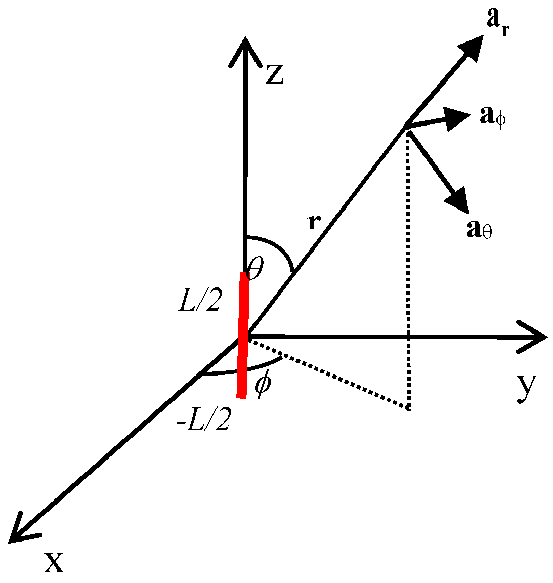
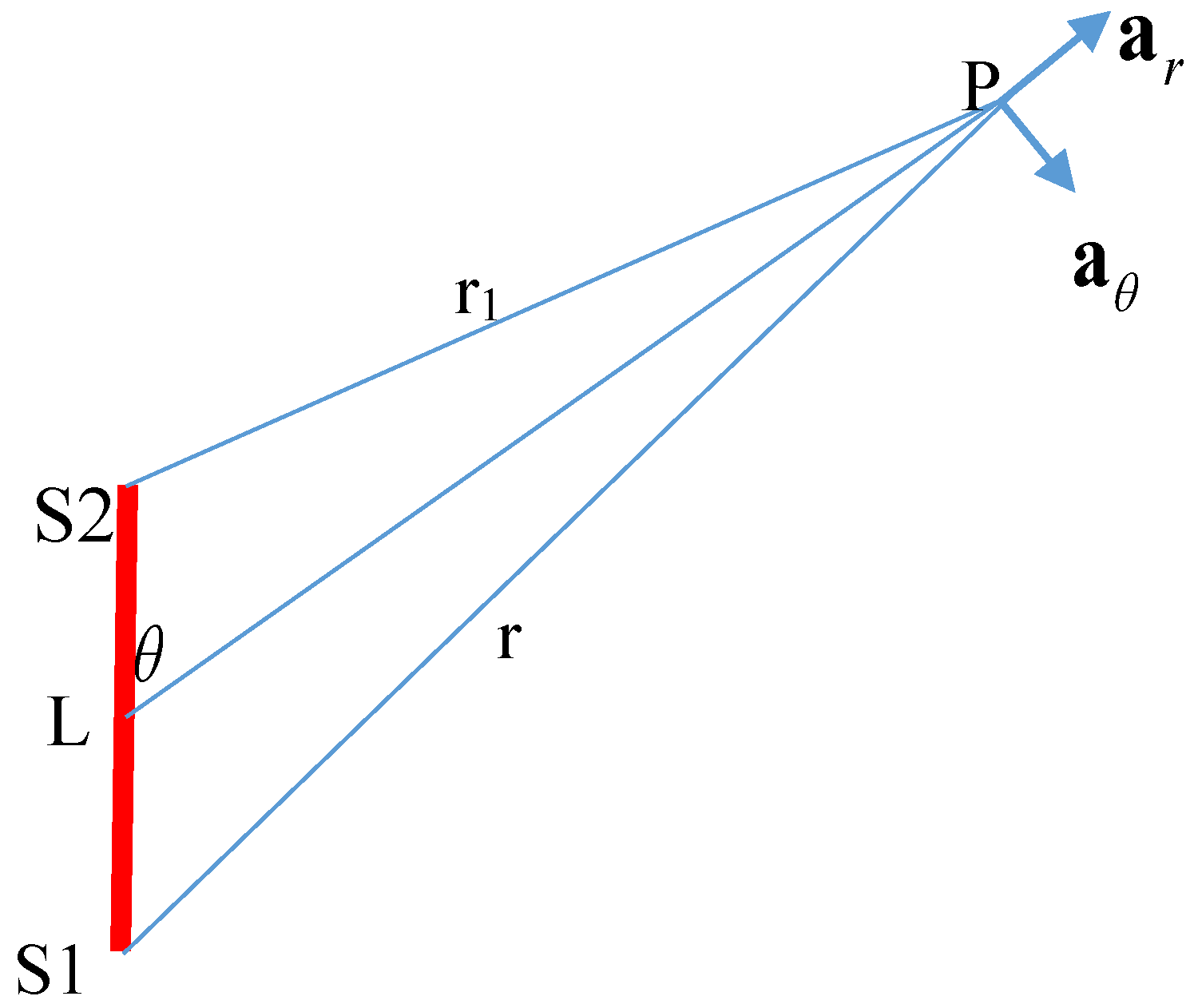
Assume that the dipole or the antenna (from here onwards, the radiating unit is referred to as the antenna) is directed along the z-axis and the origin of the axis is located at the center of the antenna. The relevant geometry is shown in
Figure 1. With this geometry, half of the antenna length is located along the positive z-axis and the other half on the negative z-axis. The z-coordinates at the two ends of the antenna are
L/2 and –
L/2. In order to calculate the electromagnetic fields, it is necessary to know the current distribution along the antenna. This information could be obtained by solving the boundary value problem using Maxwell’s equations, which is a difficult task [
5,
6]. By treating the center-fed antenna as an open circuited transmission line that has been opened out, a sinusoidal current distribution with current nodes at the ends is suggested [
5,
6]. The solution of the problem obtained by replacing the two arms of the antenna with thin ellipsoids revealed that the current is truly sinusoidal [
5]. For the cylindrical case, the assumption of a sinusoidal current is valid in the approximation when the antenna diameter is much smaller than the radius of the conductor [
5,
6] (
i.e., thin wire approximation) when the radiation damping can be neglected [
6]. A rigorous derivation of the antenna current, which indeed shows that the current distribution is sinusoidal, is presented by McDonald [
8]. Unfortunately, as the antenna length to the wavelength ratio becomes larger, the radiation damping cannot be neglected and the effect is a reduction of the amplitude of the current peaks as one moves from the center of the antenna towards its ends. On the other hand, McDonald [
8] claims that under the thin wire approximation the oscillating charges on a perfect conductor do not experience radiation damping. Calculations show that the sinusoidal current distribution is valid at least for the case when the length of the antenna is several times the wavelength of excitation [
9]. An indirect estimation can be made of the order of magnitude of the errors that may result in using the sinusoidal distribution for large
L/
λ. Chen [
10] derived an analytical equation for the transient current along an infinitely long perfectly conducting antenna excited at the center by a voltage pulse. As described by Baba and Rakov [
11], in a paper that provides a good review of the application of these concepts to return strokes of lightning flashes, this equation yields results almost identical to the exact formula given by Wu [
12]. This problem is not identical to the problem being considered here, but the analytical equation of Chen [
10] can be used to study the amount of attenuation of a sinusoidal current pulse as it propagates along the antenna. Calculations based on Chen’s formula show that the peak value of the sinusoidal current pulse can decrease by about 20% when it has travelled a distance equal to 100
λ. This shows that the maximum decrease in the peak of the sinusoidal current in the case of
L/
λ = 100 is about 20% which indicates that the deviation from the ideal sinusoidal current distribution with increasing
L/
λ is not drastic. In the calculations to be presented we will assume a sinusoidal current distribution and for the reasons given above, the results presented will be valid only up to about
L/
λ ≤ 100. However, we will show later that none of our conclusions are significantly affected by these limitations.
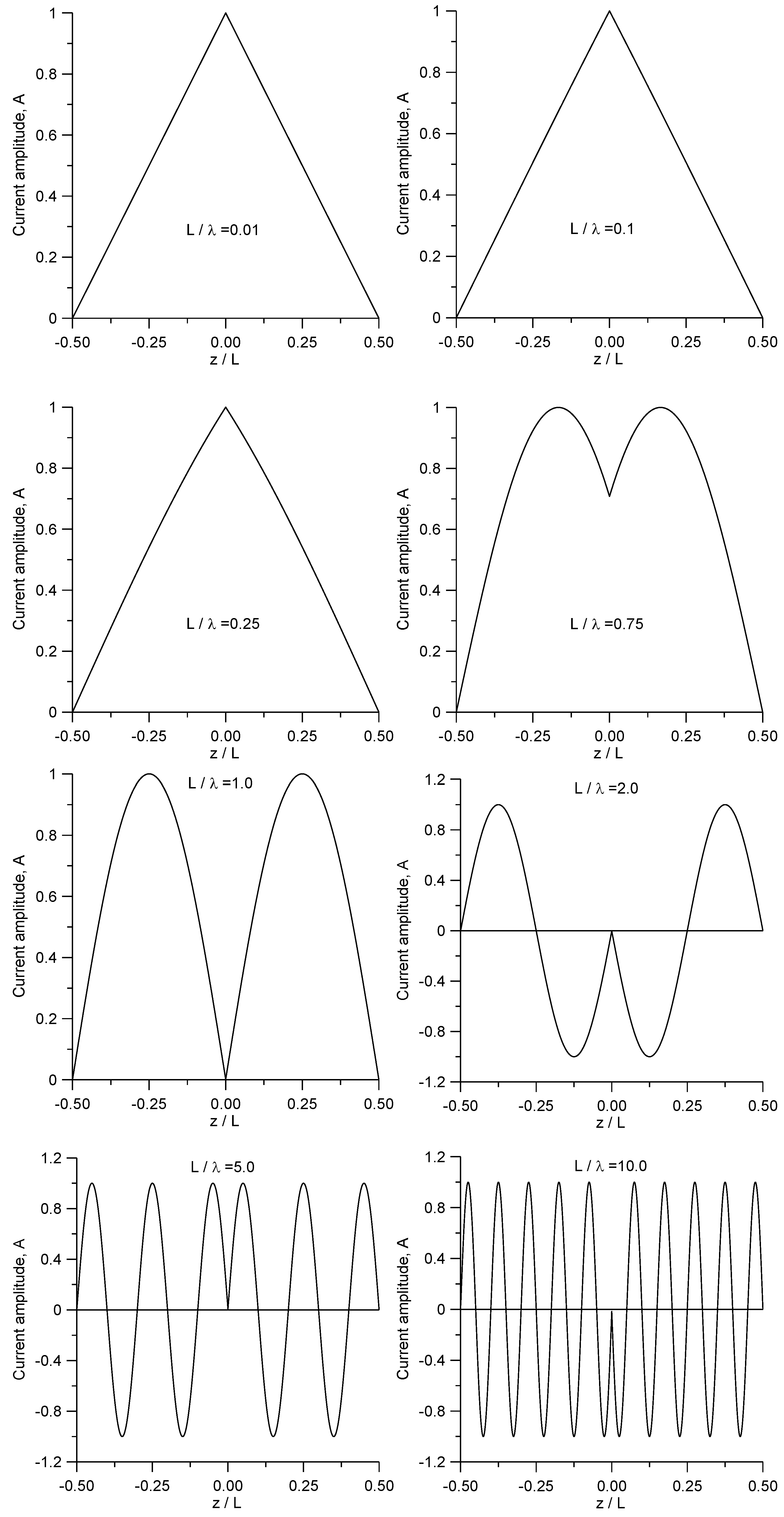
Based on the assumption of a sinusoidal current distribution, the current at any point
z on the antenna is given by [
5,
6,
13,
14]
In the above equations,
λ is the wavelength of the oscillation. The current distribution for several values of the ratio
L/
λ is shown in
Figure 2. Note that the current goes to zero at the ends of the antennas.
The radiation fields generated by an antenna excited by the current described in Equations (1) and (2) are given by [
5,
6,
13,
14]:
In the above equations
c is the speed of light in free space,
ω is the angular frequency and
k =
ω/c. We can also write down the above equation in terms of the charge oscillating in the antenna as:
In the above equations, q is the rms value of the oscillating charge in the antenna. With these equations one can calculate the power and energy produced by the antenna as a function of q and L/λ.
3. The Total Energy Transmitted by the Antenna as a Function of q and L/λ
The Poynting vector
S of the electromagnetic radiation emitted by the antenna along the radial vector is given by:
In the above equation,
аr is a unit vector defined to be in the direction of increasing
r (see
Figure 1). The energy radiated over a period of oscillation through a unit area perpendicular to the radial vector at a given distance
r, denoted by
dU, can be obtained by integrating the Poynting vector over one oscillatory period. The result is given by:
As one can see from the above equation,
dU depends not only on the angle
θ and
L/
λ but also on the frequency of oscillation and
q. In order to remove the dependence on
λ and
q, let us divide
dU by
q2 and
hν where
ν is the frequency of oscillation and
h is Planck’s constant. Note that
hν has the units of energy and, according to the quantum mechanical description, the electromagnetic radiation consists of a large number of photons with energy
hν. Once this is done we obtain:
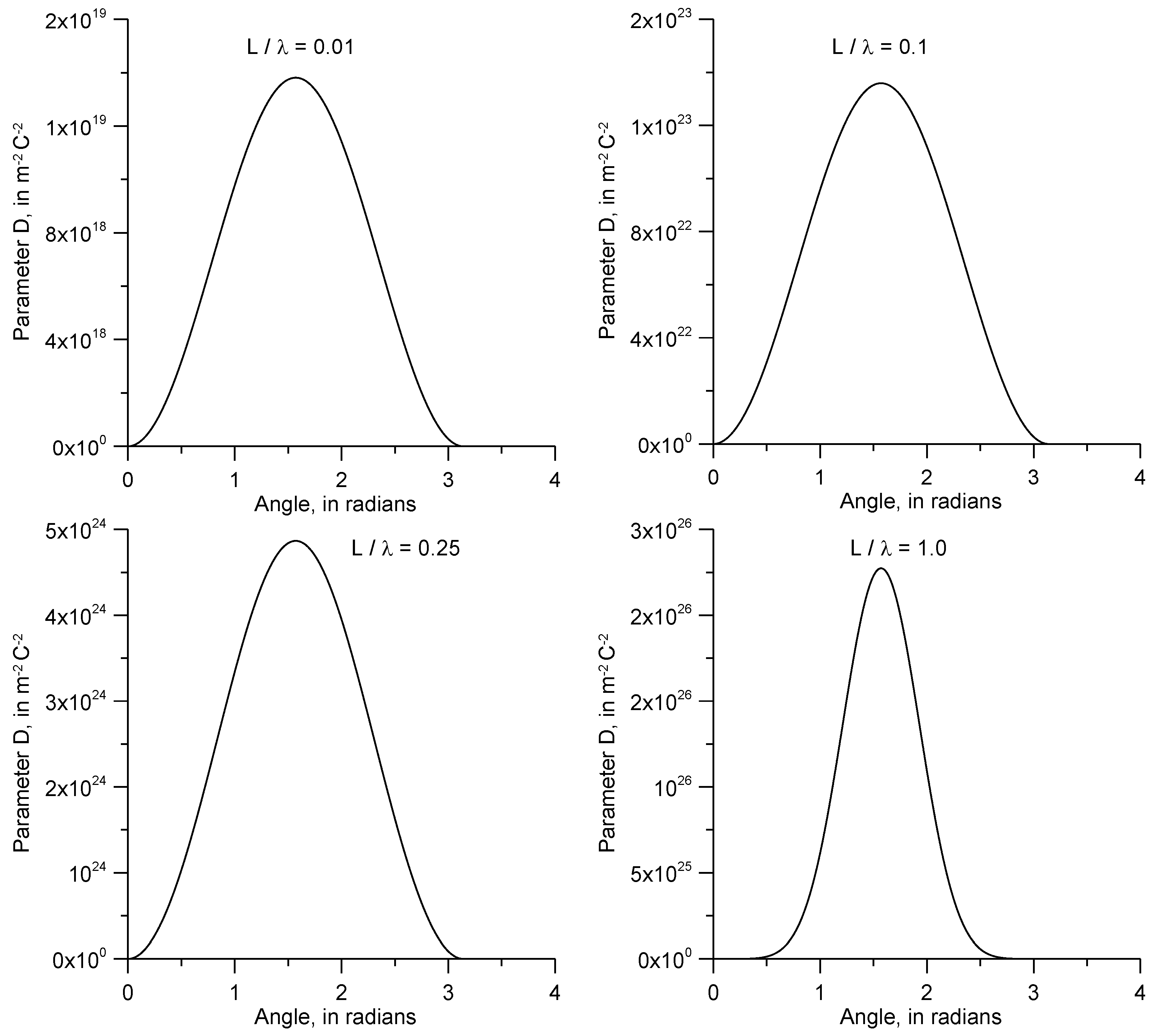
In the above equation, the parameter
D, which has the units of m
−2 C
−2, specifies how the radiation is distributed as a function of the elevation angle
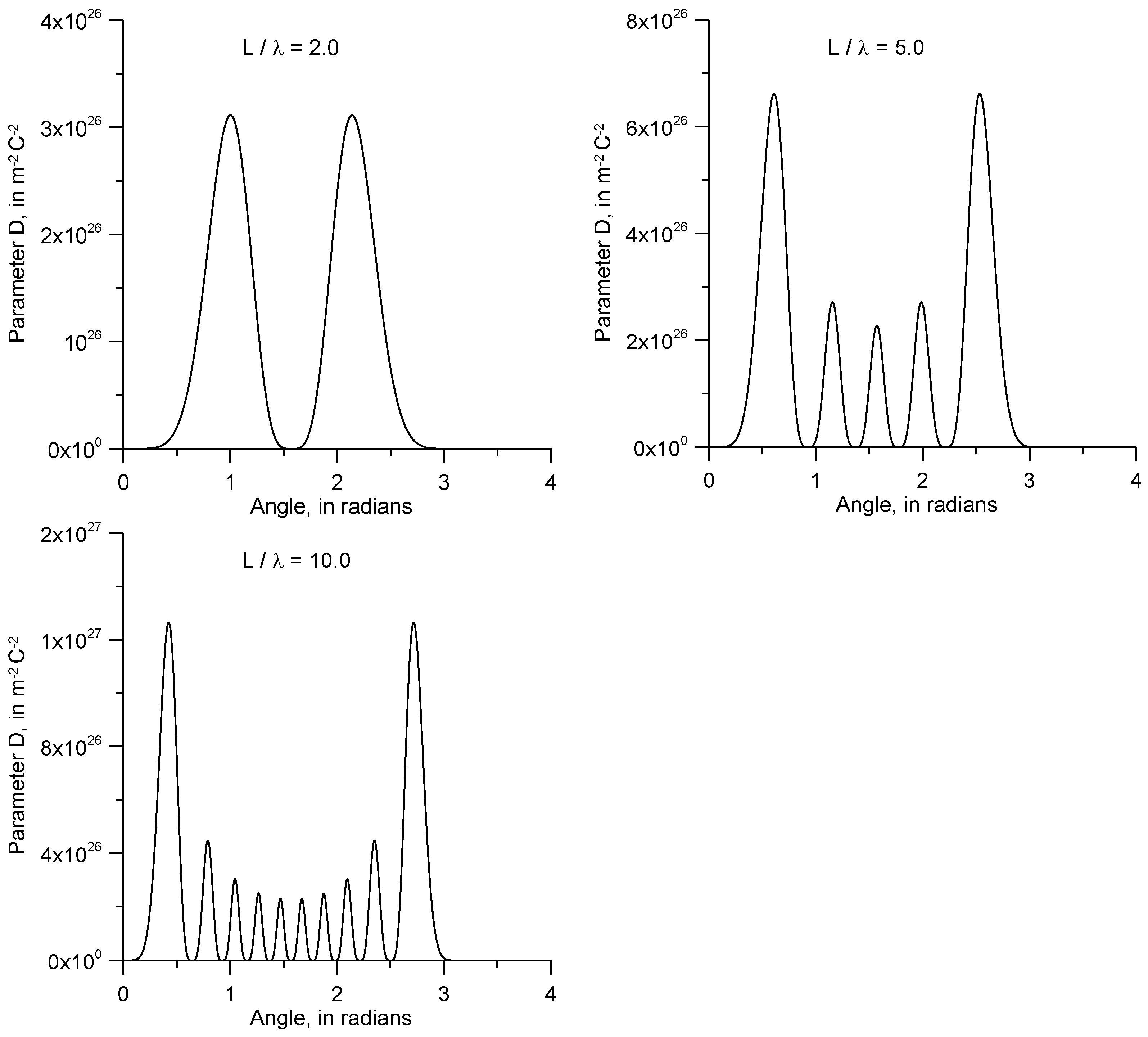
θ or its directivity. This quantity is plotted as a function of angle
θ for several values of the ratio
L/
λ in
Figure 3. In this calculation,
r = 100 km. Observe in these figures how the spatial distribution of the radiation varies as one increases
L/
λ. For very small values of this parameter, the radiation distribution is bell-shaped and it has its maximum in the direction
θ =
π/2. As
L/
λ increases, the spatial distribution of the radiation breaks into many peaks or lobes and the two largest of these move towards the angles
θ = 0 and
θ =
π. However, observe that the radiation is zero at these two angles. As
L/
λ increases further, the concentration of radiation towards these two angles becomes more and more prominent until, at extreme values of this ratio, the radiation is concentrated completely in the vicinity of
θ = 0 and
θ =
π. Notice, however, that the amplitude of the radiation is zero at these angles.
The total energy radiated by the antenna can be obtained by integrating the Poynting vector over a sphere inside which the antenna is located. Based on this, the total energy dissipated by the antenna over a period of oscillation is given by:
As before, one can normalize the energy dissipated within a period with respect to
hν and the result (denoted
Uν) is given by:
The above equation, which gives the radiated energy in units of
hν, can be physically identified as the number of photons generated within one period of oscillation. Note that
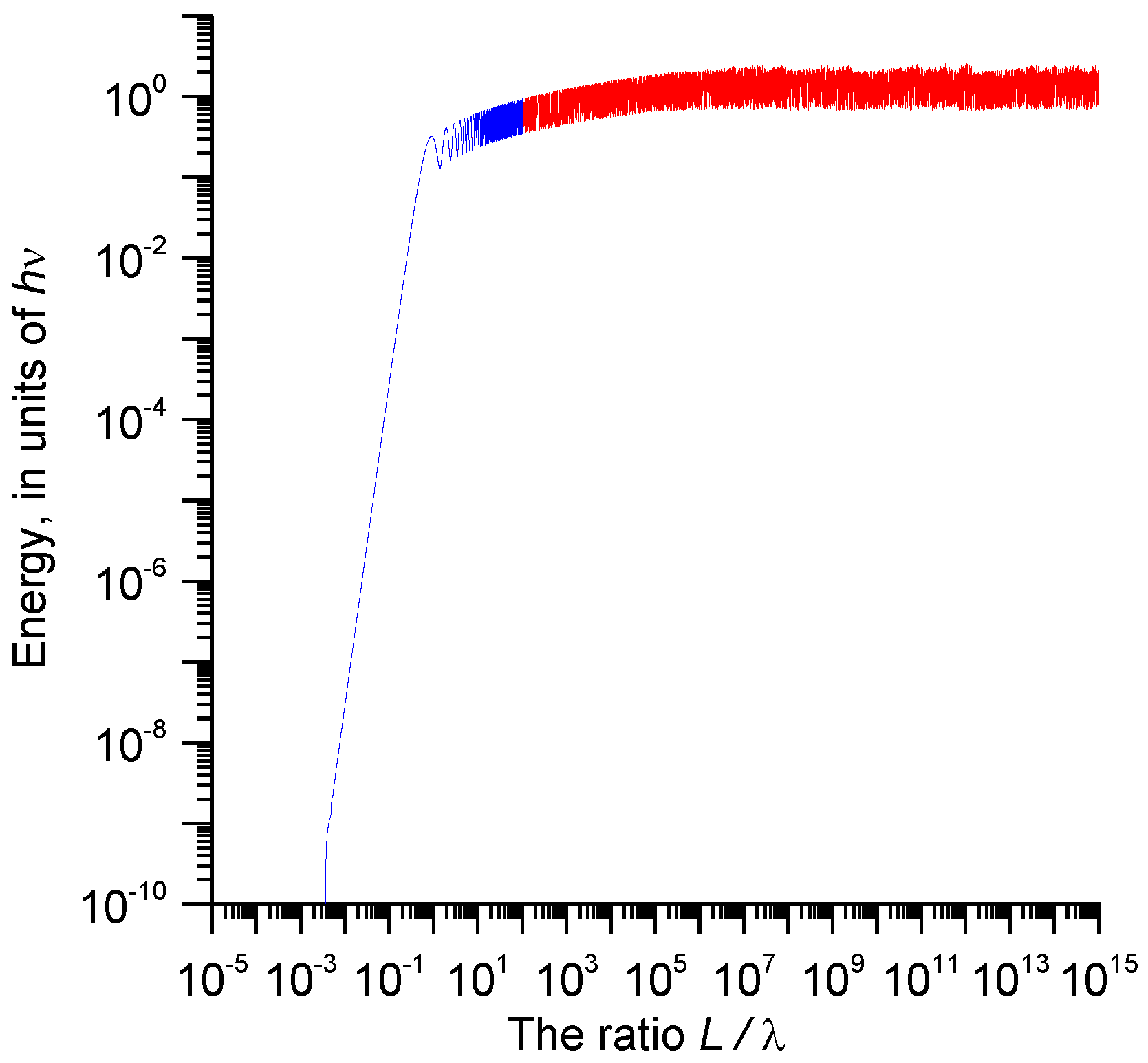
Uν increases as the square of the charge oscillating in the antenna. The values of
U as a function of
L/
λ for
q equal to electronic charge are plotted in
Figure 4. Note, also, that since the energy is proportional to the square of the charge, the energy dissipated by any other charge can be obtained readily from this graph. Observe how the energy increases initially with increasing
L/
λ and then starts to oscillate around a steady value. The amplitude of the oscillation is small compared to the steady value around which the energy oscillates. Also note the fact that, when the oscillating charge is equal to one electronic charge, the steady value of the energy is about
hν. It is important to point out that we have completely neglected the effects of radiation damping in the calculation. As mentioned earlier, the effect of radiation damping is to reduce the current peaks as one moves from the center of the antenna to the end of the antenna. This will lead to a reduction in the emitted energy for a given charge. Thus, in the presence of losses for a given charge, the energy could start decreasing with increasing
L/
λ instead of remaining constant as depicted in
Figure 4. For this reason, the plot is marked in red for values of
L/
λ larger than 100 to indicate that that region of the graph is valid only in ideal conditions (
i.e., a lossless situation) and, in reality, one may find the energy decreases with increasing
L/
λ instead of remaining constant. Observe, however, that the energy almost reaches its steady state value before reaching the region where these uncertainties become important.
Let us introduce a parameter called the action, denoted by
A, defined as the product of the energy dissipation and the time over which this energy is dissipated. That is:
where
T is the period of oscillation. This parameter, which is independent of the frequency, can be used to make a direct comparison with the time domain results to be presented in the next section. Since
T = 1/
ν, one can see from the above results that the steady state value of the action is equal to
h when the oscillating charge is equal to the electronic charge.
4. The Solution to the Analogous Time Domain Problem
The result presented in the previous section is valid for a sinusoidal current distribution along the antenna. This current distribution is derived by treating the antenna as an open-ended transmission line with the two lines opened out. The current distribution is valid for a thin conductor when the effects of radiation damping and other resistances are neglected [
5,
6]. Let us now consider the somewhat analogous problem in the time domain. If a current pulse is injected into a uniform and lossless transmission line, then the pulse will propagate at the speed of light along the line without attenuation and dispersion. Treating the return stroke as a vertical transmission line, this scenario was used by Uman and McLain [
15] to model return strokes in lightning flashes. This model, called the transmission line model, has been used very successfully to remote sense return strokes using electromagnetic fields. In this model, the return stroke is simulated by a current pulse propagating along a vertical channel with uniform speed and without attenuation. Cooray and Cooray [
16,
17] utilized this physical scenario to investigate how the energy dissipated by the radiating system varies as a function of charge. The results obtained by Cooray and Cooray [
16,
17] cannot be directly compared with those obtained in the previous section because, in their analysis, the calculated energy was normalized with respect to one of the geometrical parameters. However, they have presented all of the equations necessary for the present analysis. For this reason, the equations relevant to the radiation fields and the energy dissipated by a current pulse moving with uniform speed along a straight line are not given here in the main text. For the convenience of the reader they are presented in the
Appendix. The procedure described below is identical to the one utilized by Cooray and Cooray [
16,
17] with the exception that the net energy is studied here.
Consider a current pulse moving from one location in space to another along a straight line of length
L with constant speed
c, the speed of light in free space. The duration of the current pulse is denoted by
τ. In order to make the analysis as general as possible, the length of the current path and the duration of the current are combined into one parameter by defining
τ = βL/c, where
β is a positive constant that varies from +0 to ∞. Note that
L/
c is the time taken by the current pulse to traverse the path length
L. For a given path length, as
β varies over this range, the duration of the current waveform varies from a very small value to a very large one. Note that 1/
β can be considered to be the time domain equivalent of
L/
λ. It denotes how many ‘current lengths’ (
i.e.,
τ ×
c) can be accommodated along the path. In the analysis conducted by Cooray and Cooray [
16], the electromagnetic energy was normalized with respect to (
L/
c)/
τ. In order to make a direct comparison with the results presented in the previous section, it is necessary to consider not the normalized energy, but the net energy radiated by the system. This is what is being done here. In the present study, we assume that the propagating current pulse has a Gaussian shape and is given by:
The Gaussian current function above is normalized in such a way that
q is the total charge associated with the current pulse. In other words,
Furthermore, the peak of the Gaussian current function is shifted forward in time by 4
σ so that the amplitude and the derivative of the current pulse at
t = 0 are almost equal to zero. The duration of the Gaussian pulse can be taken as the full width at tenth of maximum (FWTM) of the pulse. This makes the duration of the current pulse,
τ, equal to about 4
σ. The variable duration of the current waveform is given by
τ =
βL/c. This makes
σ ≈
βL/4
c. All the equations necessary for the calculation of the energy and the action are given in Cooray and Cooray [
16,
17]. From the analysis in that paper (and the
Appendix of this paper), one can see directly that the energy dissipated by the current pulse can be written as:
In the above equation,
F is a function of
β and
q is the charge transported by the current. The action
A, defined as the product of the energy dissipation and Δ
t, the duration over which the energy is dissipated, is given by:
The duration over which the current pulse radiates depends on the value of
β and is given by 2
τ when
β ≤ 1 and by
τ(1 + 1/
β) for
β ≥ 1. Thus, the action is given by (see the
Appendix for further clarification)
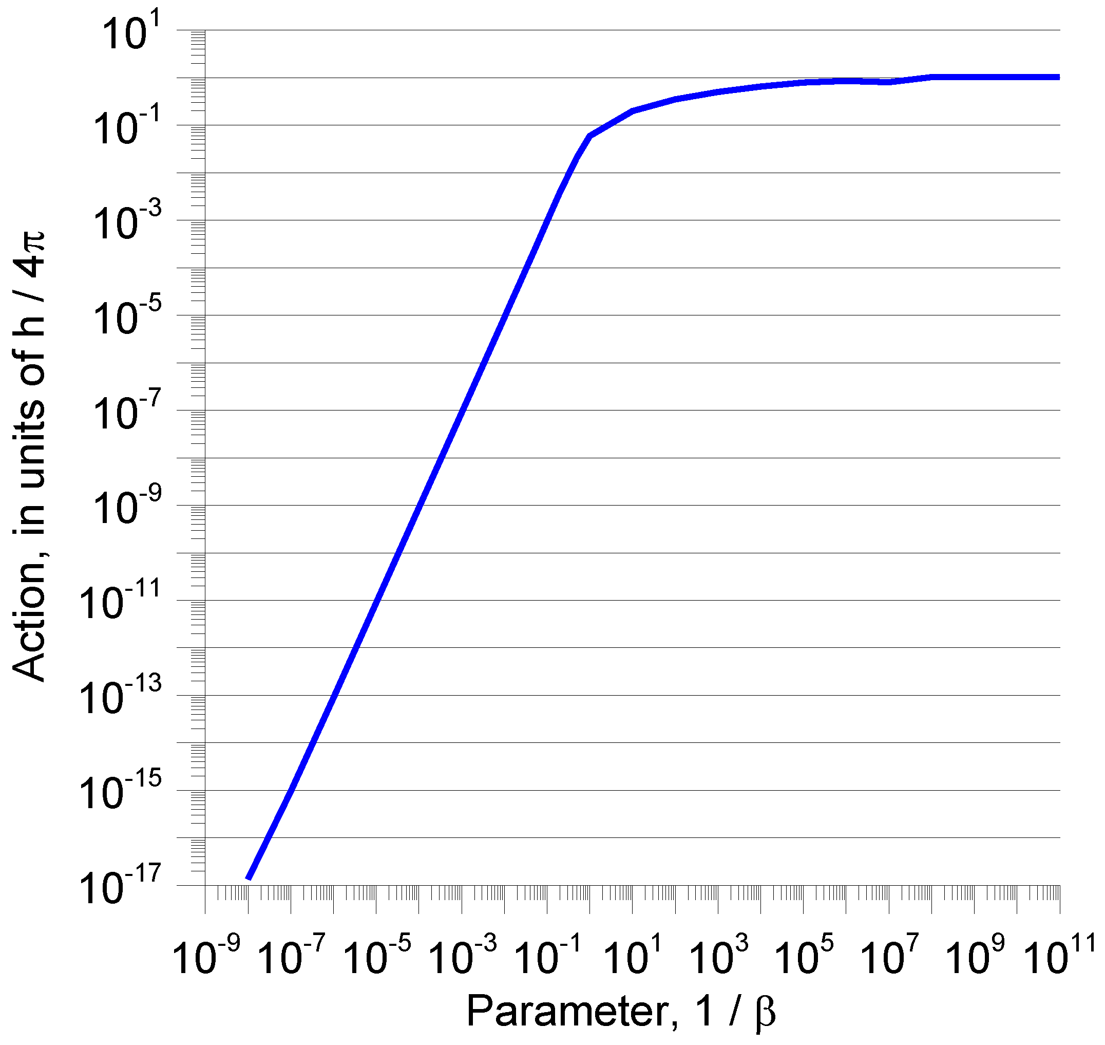
Figure 5 shows how the action varies as a function of 1/
β when the charge transported by the current is equal to one electronic charge. Since the action varies as the square of the charge, the values corresponding to other charges can also be obtained from
Figure 5. Note that, similar to the frequency domain analysis, the action reaches a steady value for large values of 1/
β. This steady value for an electronic charge is
h/4
π.
5. Discussion
Let us first consider the frequency domain results. The results presented in the previous section show that the energy dissipated by the antenna in the form of electromagnetic radiation depends strongly on
L/λ for small values of this ratio, only. As the ratio increases, the magnitude of the dissipated energy reaches a more or less steady value. Note, though, that the distribution of the radiated energy in space varies significantly with this ratio (see
Figure 3).
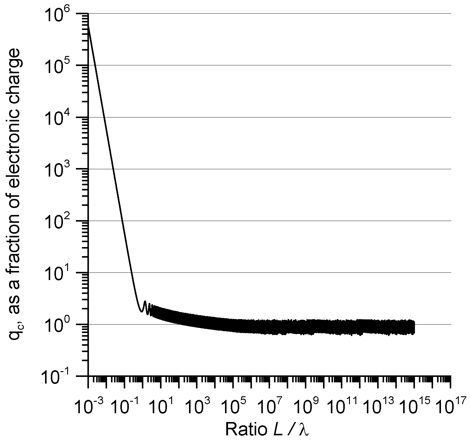
As mentioned previously, the parameter
Uν is the number of photons generated within one period by the antenna under consideration. Quantum mechanics dictates that the smallest amount of energy that can be radiated by an antenna has to be equal to or larger than
hν. An interesting question that one may ask in this respect is: what is the minimum oscillating charge, say
qc, that is necessary in a given antenna so that the energy dissipated within a period of oscillation is equal to
hν? The answer to this question is given directly by Equation (11) and it can be written as:
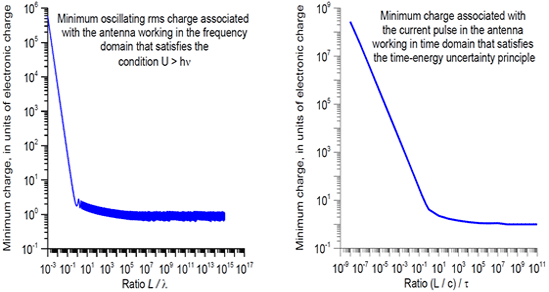
This charge (given as a fraction of the electronic charge) is plotted in
Figure 6 as a function of
L/
λ. Note how the charge decreases with increasing
L/
λ and reaches a steady value in the vicinity of the electronic charge. Now, it is reasonable to assume that the energy radiated within one period of oscillation by the antenna has to be either equal to or larger than the energy of one photon. Indeed, this energy cannot be smaller than the energy of one photon. Incorporating this fact the results can be summarized by the following mathematical expression:
That is, the condition that the electromagnetic energy dissipated over one period should be larger than the energy of a single photon corresponding to the oscillating frequency leads to the conclusion that the minimum charge that can oscillate in the antenna is larger than the electronic charge. Note, however, that the reciprocal of the above condition is not valid. That is, the condition that the oscillating charge is larger than an electron does not guarantee that the energy of the emitted radiation is larger than hν. To the best of our knowledge, this is the first time that results similar to these are presented in the literature.
It is important to recall here that the current distribution assumed in the calculation is valid only for a limited range of
L/
λ and the energy may start to decrease for large values of
L/
λ owing to radiation damping [
6,
8]. If the radiated energy starts to decrease for large values of
L/
λ, the curve in
Figure 6 would increase for large values of
L/
λ. Note, however, that the charge reaches almost an asymptotic value before reaching the region of
L/
λ where the assumed current distribution may fail as a result of radiation damping. On the other hand, the effect of radiation damping is to increase the charge for a given energy and this effect will not disturb the inequality described by Equation (20) (note the comment made in
Section 2 on radiation damping in a thin-wire antenna).
Now let us consider the time domain results. Note that the maximum value of the action when the charge in the current waveform is an electron is
h/4
π. In the case of the frequency domain results, we found that the limiting value is equal to
h. We believe, as shown later, that the factor 4
π that appears in the time domain result may have a physical significance. The result can also be interpreted as follows. First, note that electronic charge is the minimum free charge that can occur in nature. Therefore, in order to generate an action that is larger than or equal to about
h/4
π the charge associated with any current pulse has to be larger than or equal to that of an electron. In other words, one can write:
As in the case of frequency domain results, observe that the reciprocal of this relationship is not valid. That is the condition q ≥ e does not guarantee the condition .
Let us consider the physical meaning of the condition given in Equation (21). The arguments to follow are exactly identical to the ones made by Cooray and Cooray [
16] in analyzing the normalized radiated energy from a propagating current pulse. It is known that the electric charge is quantized and the smallest charge freely available is the electronic charge. Consider an experiment where an attempt is made to measure the charge transported by the current from the radiated energy using Equation (15). Under the best of conditions, the measurement of charge can be done to an accuracy of one electron. When the charge associated with the current approaches that of an electron (
i.e.,
e), the uncertainty in the measurement of the charge, say Δ
e, becomes comparable to the charge
e itself. Thus, for the electronic charge, the left hand side of the relationship given in Equation (21) can be written as:
where we have substituted for
U from Equation (15) and replaced
e2 by
eΔ
e (note that in this case
q =
e). In the case of charges larger than the electronic charge,
q >
e and Δ
q ≥ e (note that Δ
q is the uncertainty in the measurement) the above equation can be written as:
From Equation (15), one can also see that
and the above equation can be written as:
In this equation, Δ
U is the uncertainty in the electromagnetic energy and Δ
t is the duration of the emission of the radiation. This equation is identical to the earliest introduced version of the time energy uncertainty principle [
18]. One can derive a slightly different version of the time energy uncertainty principle by making the arguments as follows. When the charge associated with the current approaches that of an electron (
i.e.,
e), the uncertainty in the measurement of the energy, say Δ
Ue, becomes comparable to the energy
U itself. Thus, for the electronic charge, the left hand side of the relationship given in Equation (21) can be written as:
In the case of charges larger than the electronic charge Δ
U ≥ Δ
Ue, the above equation can be written as:
In this equation too, Δ
U is the uncertainty in the electromagnetic energy and Δ
t is the duration of the emission of the radiation.
Note that Equations (24) and (26) differ by a factor of 2. This difference arises due to the different definitions of the uncertainty in energy used in the two derivations. Actually, both these equations represent the time energy uncertainty principle in quantum mechanics. Indeed, there are several ways to derive the time-energy uncertainty principle and depending on the way it is derived the numerical factor may vary by a factor of 2. Thus, the time-energy uncertainty principle has to be considered as an order of magnitude relationship. It is important to point out here how we have defined the two parameters U and Δt in our analysis. The parameter U is the total energy radiated by the antenna and Δt is the exact time duration (as defined in Equations (A5) and (A6) of the appendix) over which the system was radiating. In other words Δt is the duration over which charges are accelerating in the system. Note that in the case of β < 1, Δt is not the time duration measured from the initiation of the first radiation burst to the end of the second radiation burst. Only with these definitions we can extract Equations (24) and (26). In our case U can also be interpreted as the total change in the energy of the system. This is the case since the radiating system is completely surrounded by the sphere over which the Poynting vector is integrated and the radiation leaving out of this sphere is the only energy that had left the system. Moreover, the parameter Δt can also be interpreted as the uncertainty in the time over which the radiation is generated for the following reasons which, of course, are partly speculative at this stage. The classical electrodynamics predicts correctly the amount of energy dissipated when the charge in the current pulse approaches that of an electron. However, at this stage the radiation may consist of a few photons and classical electrodynamics fails to predict exactly when this energy is radiated. The only statement one can make is that the energy is radiated some time during the time interval Δt during which the charge is accelerating. Thus, Δt can also be interpreted as the uncertainty in time over which the energy is dissipated.
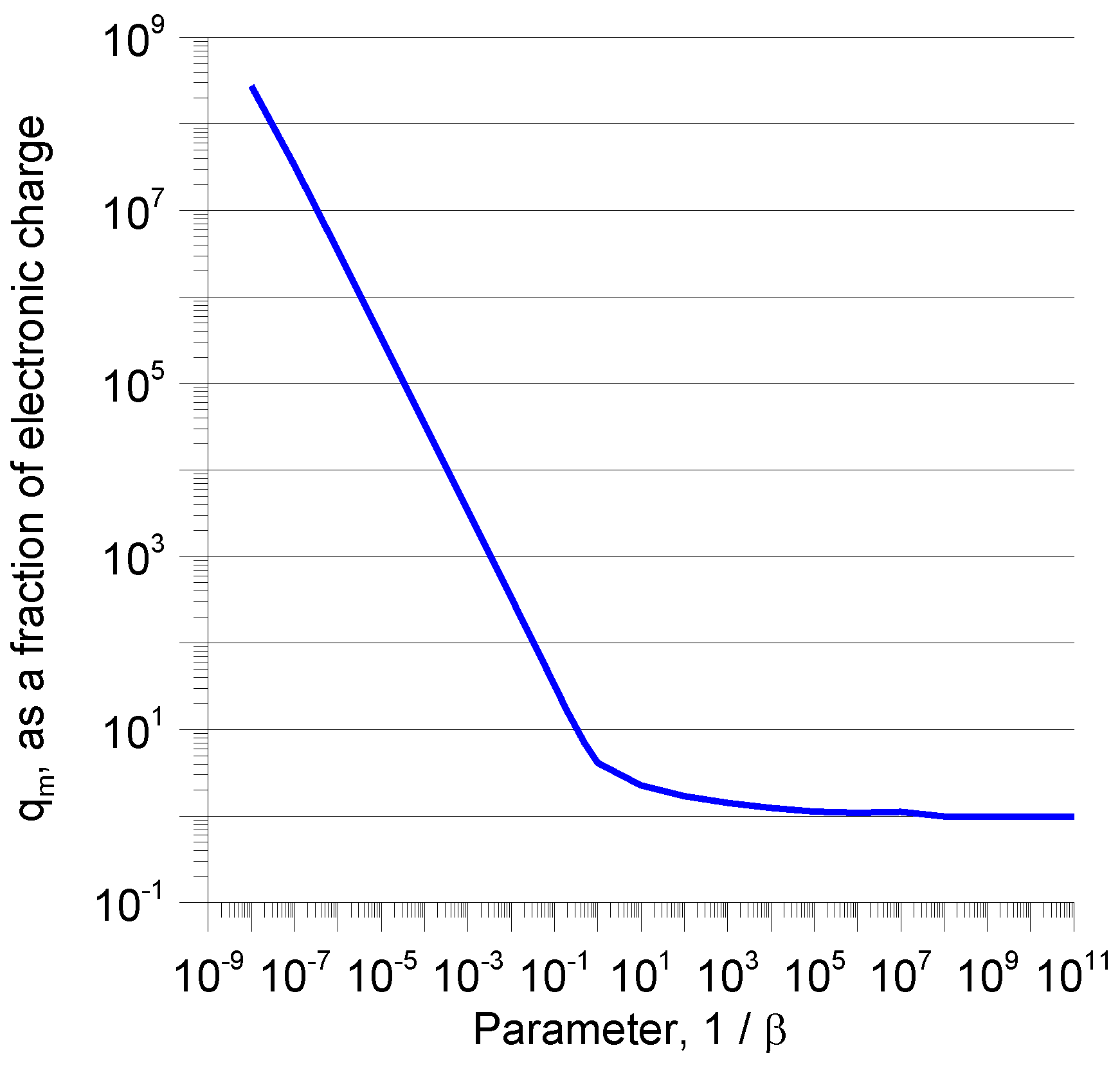
The results presented above show that the time-energy uncertainty principle is governing the fact that the smallest charge that can be detected from the electromagnetic radiation is equal to the electronic charge. For example,
Figure 7 shows the smallest charge
qm, as a function of 1/
β, associated with the current pulse required for the energy dissipation to satisfy the time-energy uncertainty principle. Note that the minimum charge that satisfies the uncertainty principle is the electronic charge. Of course, this is obvious because we have shown that Equation (21) gives rise to either Equation (24) or (26).
It is important to point out that an analysis similar to that presented above is given in the paper published recently by Cooray and Cooray [
16,
17]. The main difference is the following: In estimating the action, Cooray and Cooray [
16,
17] utilized not the net energy generated by the antenna, but the energy normalized with respect to the parameter
β. Thus, the plot of action against 1/
β is different from the one presented here. In principle, one may be able to extract the information presented in this paper from that in Reference [
16]. However, the numerical simulations conducted in that study were optimized to give a high accuracy around
β ≈ 1 where the action based on the normalized energy shows a peak and the accuracy is compromised for large values of 1/
β, making it impossible to obtain the value of the action for very large values of 1/
β. Interestingly, Cooray and Cooray [
16] came to a conclusion similar to the one reached in the present paper because the order of magnitude of the minimum detectable charge does not change when the normalized energy is used instead of the net energy in the analysis.
In this section, approximations made in the analysis of the results presented in this paper will be considered. First, consider the frequency domain results. As mentioned earlier, the approximation of sinusoidal current distribution may fail when the effect of radiation damping is taken into account. The radiation damping may start influencing the results for large values of
L/λ. As mentioned previously, the effect of this is to decrease the energy in
Figure 4 for large values of
L/λ. Fortunately, (almost) the maximum energy is reached before these effects become dominant, and for this reason, the minimum charge estimated in the analysis is not affected significantly. For this reason, we conclude that the main results presented in this paper are not affected by these effects. Moreover, as mentioned previously, the effect of radiation damping is to decrease the radiated energy for a given charge and, as a result, a higher charge is necessary to generate a given amount of energy than in the ideal lossless situation. Fortunately, this will not upset the results given by Equation (20). Let us now consider the time domain results.
In the time domain study we have neglected the attenuation and dispersion of the current pulse as it propagates along the antenna. This assumption is also made in
the transmission line model for return strokes [
15]. The effect of introducing attenuation and dispersion (
i.e., propagation losses) is to decrease the amount of energy radiated (and action) for a given charge [
16]. Fortunately, this does not affect the main conclusion as summarized by Equation (21) because a larger charge is necessary to generate a given amount of energy (and action) in the presence of losses than in the lossless case. Interestingly, this shows that the effects of losses are the same in the frequency and time domain. In the analysis we have assumed that the speed of propagation of the current pulse is equal to the speed of light. If a lower speed is used in the calculation, the amount of radiated energy will be reduced, but for the same reason as that mentioned above, it will not affect the main conclusion of this paper. The time domain analysis presented here is based on a current pulse having a Gaussian shape. The reader may wonder about the extent to which the results obtained are influenced by the temporal variation of the current waveform selected in the calculation. Our calculations (and the data presented in [
16]) show that the results remain more or less the same when other shapes (
i.e., exponential, half sinusoidal,
etc.) are used in the analysis.
The magnitude of the charge of an electron is one of the fundamental constants in nature. To the best of our knowledge no one has derived the magnitude of this charge using fundamental principles. The results presented in this paper show that the electronic charge emerges as the smallest unit of free charge in nature when the quantum mec units of h/4π) as a function of the parameter hanical constraints are applied to the radiated electromagnetic energy of a system calculated using the equations of classical electrodynamics. We hope that these calculations will provide motivation for scientists to study the two problems analyzed in this paper using quantum mechanics so that a deeper understanding can be gained as to the reason why the application of quantum mechanical constraints to the classical electromagnetic energy leads to the fact that the smallest charge that can radiate electromagnetic energy in nature is the electronic charge.


