
Estimation of Atmospheric Fossil Fuel CO2 Traced by Δ14C: Current Status and Outlook

1
School of Applied Meteorology, Nanjing University of Information Science and Technology, Nanjing 210044, China
2
Atmospheric Environment Center, Joint Laboratory for International Cooperation on Climate and Environmental Change, Ministry of Education, Nanjing University of Information Science and Technology, Nanjing 210044, China
*
Author to whom correspondence should be addressed.
Atmosphere 2022, 13(12), 2131; https://doi.org/10.3390/atmos13122131
Submission received: 25 November 2022
/
Revised: 11 December 2022
/
Accepted: 15 December 2022
/
Published: 19 December 2022
(This article belongs to the Section Atmospheric Techniques, Instruments, and Modeling)
Abstract
:Fossil fuel carbon dioxide (FFCO2) is a major source of atmospheric greenhouse gases that result in global climate change. Quantification of the atmospheric concentrations and emissions of FFCO2 is of vital importance to understand its environmental process and to formulate and evaluate the efficiency of carbon emission reduction strategies. Focusing on this topic, we summarized the state-of-the-art method to trace FFCO2 using radiocarbon (14C), and reviewed the 14CO2 measurements and the calculated FFCO2 concentrations conducted in the last two decades. With the mapped-out spatial distribution of 14CO2 values, the typical regional distribution patterns and their driving factors are discussed. The global distribution of FFCO2 concentrations is also presented, and the datasets are far fewer than 14CO2 measurements. With the combination of 14C measurements and atmospheric transport models, the FFCO2 concentration and its cross-regional transport can be well interpreted. Recent progress in inverse methods can further constrain emission inventories well, providing an independent verification method for emission control strategies. This article reviewed the latest developments in the estimation of FFCO2 and discussed the urgent requirements for the control of FFCO2 according to the current situation of climate change.
1. Introduction
Carbon dioxide (CO2), the most important greenhouse gas, is a significant driver of global warming. In 2019, the annual average concentration of CO2 reached 410 ppm, which was higher than any time in at least 2 million years [1]. The observed increase in CO2 concentrations since the beginning of the industrial era is unequivocally caused by human activities, among which the combustion of fossil fuels is responsible for most of the total anthropogenic CO2 emissions. Global warming has caused increases in the global temperature of the surface and upper ocean, increases in precipitation and sea level, weather, and climate extremes, and decreases in glaciers and sea ice [2,3,4,5]. Besides CO2, fossil fuel combustion is also a primary contributor to air pollutants [6]. Thus, slowing down the increase in fossil fuel CO2 (FFCO2) concentration is of vital importance. According to the Paris Agreement and the sixth assessment report of IPCC (Intergovernmental Panel on Climate Change), CO2 emissions need to be net negative to hold the global surface temperature lower than 1.5 °C or 2 °C at the end of this century (very low and low greenhouse gas emission scenarios, according to IPCC, 2021). This means that the anthropogenic removal of CO2 exceed anthropogenic emissions. Under these circumstances, identifying the contribution of FFCO2 to total atmospheric CO2, as well as its atmospheric process interpretation and emission estimation, is a fundamental work for studies on its climatic and environmental impacts and on the evaluation of mitigation actions.
Multiple tracers that co-emitted with CO2 have been used to quantify FFCO2, including carbon monoxide (CO), sulfur hexafluoride (SF6), tetrachloroethylene (C2Cl4) and even air pollutants, based on the ratio of each tracer to CO2 [7,8,9,10,11,12,13,14]. However, there are large uncertainties due to the non-fossil emissions of the tracers [15]. Radiocarbon (14C), a widely used dating method in archaeology, geosciences, etc. [16], is a direct tracer and a promising method to differentiate the emissions of fossil fuel and non-fossil fuel from atmospheric carbon. The abundances of three naturally occurring carbon isotopes 12C, 13C and 14C are 98.89%, 1.11%, and ~10−10%, respectively [17]. The radiocarbon content of CO2 is expressed as Δ14C or Δ14CO2 [18,19]:
(14C/12C)SN is the 14C to 12C ratio of the sample, and (14C/12C)ABS is related to the commonly used primary measurement standard Oxalic Acid I. Radiocarbon is cosmogenic, and has a radioactive half-life of 5730 ± 40 years [20]. Thus, there are no 14C in fossil fuels because they are all depleted during long-term radioactive decay. Since fossil fuel CO2 contains no 14C whereas CO2 from other sources has similar 14C concentrations with the ambient air, the release of fossil fuel CO2 will cause a decrease in the 14C/12C ratio in the atmosphere. This was first discovered by Hans Suess [21], and is called the “Suess effect”. With industrial development, atmospheric Δ14CO2 decreased by 25‰ between 1890 and 1950 [22]. Then comes the nuclear testing period between the 1950s and the early 1960s, during which large-scale detonations of nuclear bombs produced 14C atoms in the Northern Hemisphere. Atmospheric Δ14CO2 in the Northern Hemisphere increased swiftly and reached a peak value of nearly 1000‰ in 1963, and then decreased after the Limited Nuclear Test Ban Treaty [23,24]. In addition to those mentioned above, other principal influence factors on Δ14CO2, include interhemispheric transport, ocean circulation, nuclear power plants and terrestrial biosphere, will be discussed later.
In this review, we focus on the newly added FFCO2 traced by 14C, mainly present progress in the 21st century. We first present the commonly used method of Δ14CO2 sampling and measuring, as well as the basic theory of FFCO2 calculation (Section 2). Then, we summarize the atmospheric Δ14CO2 trend in several representative background sites, which is essential to the calculation of FFCO2 (Section 3). In Section 4, we reviewed the measurements of Δ14CO2 and the calculated FFCO2 concentrations globally and present the spatial patterns and temporal variations. The recent progress of the combination of 14C measurements and atmospheric transport models to interpret FFCO2 concentration and its cross-regional transport, and to estimate the emissions of FFCO2, are also reviewed.
2. The Basis of Tracing Fossil Fuel CO2 Using 14C
2.1. The Theory of Quantifying Fossil Fuel CO2 Using 14C
Observed CO2 mole fraction (or concentration) is thought to be a mixing of many components, mainly including atmospheric background CO2, fossil fuel CO2, biospheric CO2 and oceanic CO2. The most commonly used method to constrain recently added FFCO2 in the atmosphere with 14C is called the pseudo-Lagrangian method [25,26,27], in which a parcel of air with an initial CO2 mixing ratio (CO2bg) and Δ14CO2 value (Δbg) moves across a polluted region, and then CO2 mixing ratio and Δ14CO2 value are modified to CO2obs and Δobs by the addition of FFCO2 and other sources or sinks of CO2. If combining other sources (and sinks) together, the mixing ratio and the Δ14CO2 value could be written as CO2other and Δother. Two balance equations for CO2 mixing ratio and Δ14C can be formulated as below.
By combining Equations (2) and (3), CO2ff can be calculated as:
CO2obs, Δobs are measured in collected samples at interested sites. Δbg is measured in samples from background sites in general, while free tropospheric measurements can also act as Δbg, too [13]. Δff is known to be −1000‰ since CO2ff is 14C-free.
The second term of Equation (4) is bias due to the effect of the others:
some researchers assume β to be zero, which means that all other sources have the same Δ14C compared to those of the background atmosphere, Δother = Δbg [26]. The main contributor to uncertainties in β would be heterotrophic respiration, which has large 14C disequilibrium. The ignorance of β would cause a systematic underestimation of CO2ff, up to 0.5 ppm in summer and 0.2 ppm in winter [13,27]. There are two other factors that influence atmospheric Δ14CO2, air-sea exchange in the oceans, and stratosphere-troposphere transport [28]. However, these exchanges are assumed to affect the background and observed samples equally; thus, normally, they will not be counted in the calculation of FFCO2.
2.2. Air Sampling and Measurement
Atmospheric Δ14CO2 can be measured with direct air sampling. Whole air samples are normally collected using flasks or bags. Short-period and integrated samples can be collected by pump and acid solution, respectively. CO2 samples can be collected by static absorption using CO2-free sodium hydroxide (NaOH) or barium hydroxide (BaOH) solutions in flasks [25,29,30]. The primary collection method is the static absorption of CO2 using CO2-free sodium hydroxide (NaOH) or barium hydroxide (BaOH) solutions in discrete glass flasks [25,29]. The flasks are exposed to air for collection of integrated samples. Besides ground sites, tall towers, aircrafts, balloons, and even kites are all effective platforms to collect CO2 samples [13,31,32,33,34].
Air samples reflect near real-time atmospheric Δ14CO2, can be used to characterize the FFCO2 temporal variations with high resolution effectively. However, the representativeness of the air samples is limited to those of the sampling region and period, while little information (spatial and temporal distribution) is known beyond that. In addition, the sample collecting process and/or the site maintenance is labor and cost intensive. Direct sampling of air is not the only way to analyze atmospheric Δ14CO2. Plants fix CO2 from the atmosphere via photosynthesis, offering a unique complementary analysis method.
For plants, their carbon isotopic composition can be used to reflect the mean atmosphere Δ14CO2 isotopic composition of their growing period. By collecting plant samples in different regions and analyzing 14C, FFCO2 spatial distribution on a large scale can be mapped out. Compared to air samples, collecting plant materials is more convenient and relatively cheap. Tree rings and annual leaves (grasses) are two main types used to reveal the spatiotemporal distribution of FFCO2 [30,35,36,37,38,39,40]. Each plant species may have its own advantages in addition to those illustrated above. Maize is grown in many countries, so it is convenient to map out the large-scale spatial distribution of fossil fuel influences using corn leaves. Gingko is a perennial and deciduous tree that is widely planted in East Asian countries, urban areas, and rural areas. Thus, it is feasible to separate samples of clean sites from samples of polluted sites. Wine ethanol is a unique plant material that can represent previous sampling years, since the harvest year and region are all written on the label of the wine bottle. Tree rings, a unique plant material, help in the reconstruction of annual atmospheric Δ14CO2 for decades or hundreds of years. In practice, however, the sampling of tree rings may be more difficult than that of annual plants since it is difficult to separate one annual ring from the others.
Comparisons of Δ14CO2 and/or FFCO2 between plant materials and air samples show nearly consistent results [30,41,42,43], which verifies the usage of plant materials. Xiong et al. [44] found a significant difference in Δ14CO2 between respired CO2 and bulk organic matter from 21 plant species, suggesting that bias associated with dark respiration should be considered when use 14C in plants to quantify atmospheric FFCO2. It should be noted that biomass accumulated by plants only represents daytime Δ14CO2 (when photosynthesis occurs), and the sampling should be well planned for different plant species considering their growing period and local climate.
Before the analysis of 14C, the preparations of air samples included extracting the CO2 (purification), and the reduction of CO2 to graphite. The extraction of CO2 is to remove water cryogenically, freeze CO2 completely together with N2O (non-interfering), and without freeze O2 or CH4 [13,45]. Graphite is produced by adding hydrogen gas to CO2 over an iron catalyst [46,47]. The atom counting of each graphite sample is then performed by an accelerator mass spectrometer (AMS). The preparation of annual leaves is a little different from air samples: plant samples need to (1) be cleaned by pure water and then dried, (2) be combusted to CO2 and then reduced to graphite [35].
Direct atom-counting of 14C using AMS is a great progress of 14C analysis methods. Before that, the conventional methods were decay counting, solid carbon using a Geiger–Muller counter, and liquid scintillation counting [48]. The sensitivity was improved around 106 times by AMS over the decay counting methods [49]. With the attempts to reduce sample size and to increase precision, the detection limits have been reduced to ~5 µg of carbon [50,51], and the reported precisions have reached 1‰ [17].
3. Atmospheric Δ14CO2 Trend in Background Sites
To characterize the newly added atmospheric FFCO2, it is necessary to first study the Δ14CO2 variations at background sites. Background sites are located in remote areas (high mountain, coastal area, etc.), rarely influenced by local pollution. When analyzing Δ14CO2 values from certain sites to deduce the contribution of local or regional fossil fuels, Δ14CO2 measured at background sites helps separate it from continental trends. In this study, we summarize the background Δ14CO2 measurements in the last two decades from six representative background sites, including Jungfraujoch and Schauinsland (Europe), Niwot Ridge and La Jolla (North America), Waliguan (Asia), and Wellington (Oceania) (Figure 1).
In Europe, Jungfraujoch (JFJ) and Schauinsland (SIL) are the two most representative background sites. Jungfraujoch is located in the Swiss Alps at an elevation of 3450 m a.s.l. and mostly samples air from the free troposphere over [59]. Schauinsland is in Black Forest, Germany, with an elevation of 1205 m a.s.l. Schauinsland normally samples free tropospheric air during the night but is influenced by boundary layer air during the day [60]. The two stations all use 2-week integrated CO2 samples collected by NaOH solution absorption. Levin et al. [53] found Δ14CO2 in both sites showed a steady decreasing trend, about 6‰ per year at the beginning of the 21st century and 3‰ per year on average in 2009–2012. The seasonal features of Δ14CO2, they are similar for nearly all the background sites, with maxima recorded during summer/autumn and minima during winter/spring.
Niwot Ridge (NWR), Colorado, USA, has a high elevation (3475 m a.s.l.) continental site, can be used as a proxy for North American free tropospheric air [56]. The measurement of Δ14CO2 began in 2003 using whole air samples. According to Turnbull et al. [56], Δ14CO2 at NWR decreased by 5.7‰ per year from 2004 to 2006, with a seasonal amplitude of 3–5‰. Lehman et al. [55] extend the dataset to 2011. Measurement in La Jolla, California, is conducted at the Scripps Pier, using whole air samples when meteorological conditions are favorable for collecting clean marine air [54]. The monthly samples show a decreasing trend of 5 ± 0.2‰ per year from 2001 to 2007. The decreasing trends in North American background sites are similar to the two European stations. NWR appears to be a reasonable choice of background air for Northern Hemisphere midlatitude and has been used as background CO2 and Δ14CO2 to quantify FFCO2 [27,58].
Compared to Europe and North America, the measurements of Δ14CO2 in Asian sites are not continuous. Waliguan (WLG) Global Atmosphere Watch (GAW) station, located on top of Mt. Waliguan (3816 m a.s.l.), the northeast part of the Qinghai-Tibetan Plateau, represents the background air for the Eurasian continent. Since Δ14CO2 is not measured conventionally on this site, there is only a small amount of data [57,58]. Δ14CO2 values at WLG during 2004/2005 are close to those measured at NWR [58]. Even though the values of WLG in 2015 are lower than the other background sites in previous years, they may be similar considering the annual trend at other sites. The observations at some regional background sites in China are also shown in Figure 1, all collected during a short period and mostly lower than the values in the WLG [9].
The world’s longest direct record of atmospheric Δ14CO2 was begun at Wellington, New Zealand, in 1954 [52,61]. The sampling sites in Wellington are located in the coastal areas of two islands. Through decades of measurement, the collection method and measurement method have changed several times (details in [52]). In the 21st century, Δ14CO2 in Wellington is consistently higher than in Northern Hemispheric sites, as shown in Figure 1. Based on seven global stations, Graven et al. [28] found that the mean Δ14CO2 in the Northern Hemisphere was 5‰ lower than that in the Southern Hemisphere over 2005–2007. The interhemispheric exchange time is estimated to be 1.4 years [56,62]. Many researchers have interpreted these contributions to the interhemispheric gradient [24,28,52]. The major cause includes the dilution by 14C-free fossil fuel emissions in the north, and the weakening of 14C-depleted ocean upwelling in the south. The oceans are the largest reservoir of carbon, and the principal natural drivers that are responsible for atmospheric Δ14CO2. Air-sea 14C flux is greatly influenced by ocean circulation and atmosphere-ocean CO2 exchange. The reducing 14C uptake and the weakening 14C-depleted upwelling in the Southern Ocean resulted in a decrease in atmospheric Δ14CO2 [24].
Among all background sites, the annual decreasing trends of Δ14CO2 in the 21st century are similar. According to the observations and modeling conducted by Levin et al. [24], the global long-term trend in Δ14CO2 is main influenced by fossil fuel emissions since the 1990s. If fossil fuel emissions continue to increase in a “business-as-usual” scenario in the IPCC Fifth Assessment Report, Δ14CO2 will likely drop below the preindustrial level (0‰) in a decade and be reduced to −250‰ by the year 2100. However, if ambitious emission reductions could be conducted, Δ14CO2 will be sustained near the preindustrial level through 2100 [63].
In general, it is recommended that the quantification of FFCO2 need to refer to the corresponding background Δ14CO2 values and CO2 concentrations, due to the spatial gradients in Δ14CO2. However, Turnbull et al. [58] estimated FFCO2 in South Korea with four different background sites (WLG, NWR, Mauna Loa, Hawaii, and Ulaan Uul, Mongolia) separately, and found no substantial change in the results. The enhancements above baseline are typically large compared to the differences caused by the choice of background.
4. Spatial and Temporal Variations of Δ14CO2 and FFCO2
To provide a periodical review of the spatiotemporal characteristics of FFCO2, we collected Δ14CO2 measurements of air and plant samples and/or the calculated FFCO2 reported in the past two decades (Table 1). Since measurements in Europe and North America have been implemented for decades, we focus more on the recent measurements in Asia (Figure 2, where CO2 emissions are higher than in other regions [64]). The global FFCO2 distribution is plotted in Figure 3.

Table 1.
Δ14CO2 measurements and calculated FFCO2 concentrations reported in the last two decades.
| Location | Sampling Period | 14CO2 (‰) | FFCO2 (ppm by Defult) | Site Type/Name | Note (Air Samples with No Notes) | References | |
|---|---|---|---|---|---|---|---|
| Hungary | September 2008–April 2009 | −4.5~39.1 | city | [65,66] | |||
| 23.1~48.1 | rural (10 m) | ||||||
| 31.4~47.3 | rural (115 m) | ||||||
| Netherlands | 2010–2012 | 35.2, 27.2, 22.6 | corn leaves | [42] | |||
| Germany | 2012 | 17.2 | |||||
| France | 2012 | 31.7 | |||||
| Poland | July 2011–May 2013 | −178.2~4.7 | 66.6~72.7% | [43] | |||
| Romania | August 2012–January 2018 | –57~61 | industrial area | [67] | |||
| Switzerland | June 2013–December 2015 | 4.3 | tall tower | [7] | |||
| England | June 2014–August 2015 | −35.26~59.61 | −1.09~2.27 | tall tower | [68] | ||
| North America | 2004, summer | 66.3 ± 1.7 |
mountain regions,
western North America | corn leaves | [35] | ||
| 58.5 ± 3.9 | 2.7 ± 1.5 | eastern North America | |||||
| 55.2 ± 2.3 | 4.3 ± 1.0 | Ohio-Maryland region | |||||
| California, USA | 2004–2005 | 59.5 ± 2.5 | 0.3 ± 0.08 | North Coast | annual C3 grasses | [37] | |
| 44 ± 10.9 | 6.1 ± 1.1 | San Francisco | |||||
| 48.7 ± 1.9 | 4.8 ± 0.9 | Central Valley | |||||
| 27.7 ± 20 | 13.7 ± 0.4 | Los Angeles | |||||
| Los Angeles, USA | 2006–2013 | −59.4~29.3 | inland Pasadena | [69] | |||
| 2009–2013 | −18.8~40.4 | coastal Palos Verdes | |||||
| high latitudes, | 2008 | spring | 46.6 ± 4.4 | flight | [70] | ||
| North America | summer | 51.5 ± 5 | |||||
| central California, USA | 2009–2012 | winter | 7.2 | Walnut Grove | [71] | ||
| spring | 3.1 | ||||||
| summer | 3.7 | ||||||
| fall | 5.0 | ||||||
|
southern California,
USA | 2013–2014 | winter | 25 | California Institute of Technology in Pasadena | |||
| spring | 21.6 | ||||||
| summer | 25.9 | ||||||
| fall | 21.5 | ||||||
| winter | 8.2 | San Bernardino | |||||
| spring | 5.1 | ||||||
| summer | 11 | ||||||
| fall | 10.2 | ||||||
| Mexico City | March 2006 | 20~132 | [72] | ||||
| South Korea | 2009 | −112.3~−12.4 | 4.2~13.9 | Seoul, metropolitan area | gingko leaves | [73] | |
| −79.5~43.8 | −1.3~10.7 | Busan, metropolitan area | |||||
| –69.3~28.1 | 0.2~9.7 | Daegu, metropolitan area | |||||
| −53.4~−2 | 3.2~8.2 | Daejeon, metropolitan area | |||||
| −41.7~19.2 | 1.1~7 | Gwangju, metropolitan area | |||||
| South Korea | 2009 | 34.8 | clean air sites | gingko leaves | [38] | ||
| 2010 | 24.9 | ||||||
| 2011 | 23.1 | ||||||
| 2012 | 14 | ||||||
| 2013 | 8.3 | ||||||
| Anmyeondo, South Korea | May 2014–August 2016 | −59.5~23.1 | 9.7 ± 7.8 | [9] | |||
| Tae-Ahn Peninsula, | 2004–2010 | all year | 4.4, 60% | [58] | |||
| South Korea | winter | 4.4, 90% | |||||
| Beijing | March 2009–September 2009 | 3.4 ± 11.8 | 16.4 ± 4.9 | [74] | |||
| 12.8 ± 3.1 | suburban sites | ||||||
| −8.4 ± 18.1 | road sites | ||||||
| 2009 | −28.2~29.6 | corn leaves | [75] | ||||
| 2014 | −53.5 ± 54.8 | 39.7 ± 36.1, 75.2 ± 14.6% | urban site | [76] | |||
| Guangzhou | 2010–2011 | –16.4 ± 3.0 | 24 (1–58) | [77] | |||
| Xiamen | 2014 | −8.7 ± 25.3 | 13.6 ± 12.3, 59.1 ± 26.8% | urban site | [76] | ||
| Xi’an | March 2012–March 2013 | −41.3 ± 27.4 | [30] | ||||
| April 2012 | −9.7 ± 23.8 | ||||||
| January 2013 | −90.4 ± 32.4 | ||||||
| March 2012.03–March 2013 | 34.2 ± 9.5 | ||||||
| March 2012–March 2013 | winter | 46.5 ± 8.7 | |||||
| March 2012–March 2013 | summer | 26.6 ± 3.4 | |||||
| Xi’an | 2013 | summer | 20.5 | annual plants | [78] | ||
| 2014 | summer | 23.5 | |||||
| Xi’an | 2014 | winter | 92.7 ± 9.7 | [79] | |||
| 2016 | winter | 61.8 ± 10.6 | urban | [80] | |||
| 2016 | winter | 57.4 ± 9.7 | suburban | ||||
| 2016 | summer | 82.5 ± 23.8 | urban | ||||
| 2016 | summer | 90 ± 24.8 | suburban | ||||
| Bali, Indonesia | September 2018 | 2.2 ± 19 | 6.4 ± 7.5 | evergreen leaves | [81] | ||
Figure 3.
The spatial distribution of Δ14CO2 traced FFCO2. The percentage in pie charts represents the fossil fuel component to total CO2. The grid lines in histograms represent that the FFCO2 value is 50 ppm. Colors in pie charts and histograms: blue-spring, green-summer, orange-autumn, red-winter, black- yearly values [7,9,35,37,43,58,71,74,76,77,79,80,83].

4.1. Spatial Patterns of Δ14CO2 and FFCO2
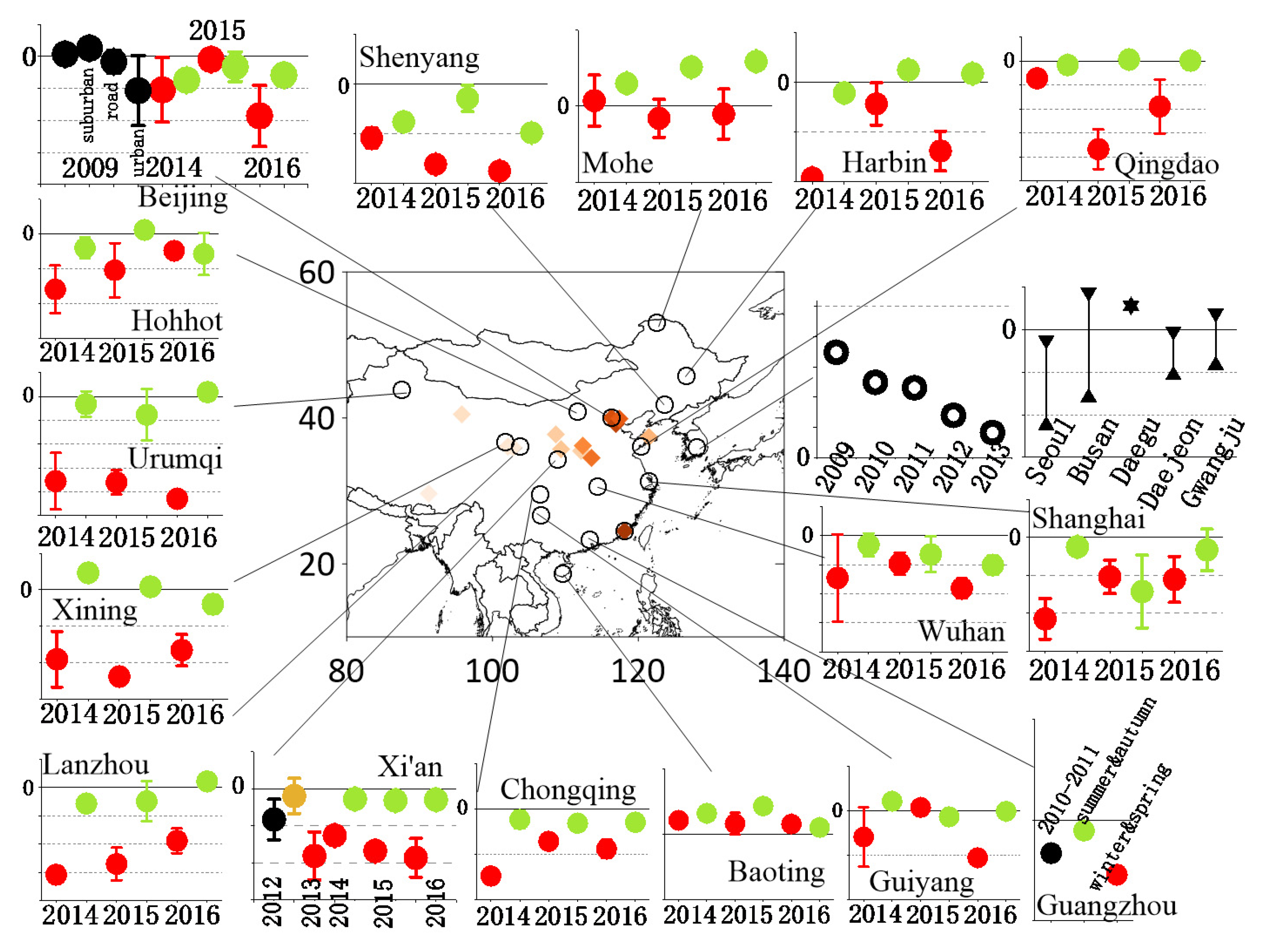
Δ14CO2 measurements in Asia are mostly carried out in China, South Korea, and Japan around the 2010s. There are great differences in Δ14CO2 values among cities. Highest Δ14CO2 values appear in cities in middle and western China (light orange diamonds in Figure 2), where are sparsely populated. The Δ14CO2 values measured in Northeast China (Mohe, Harbin, and Shenyang) and in coastal areas (Baoting, Xiamen, and Guangzhou) are also higher than those in other cities. Lower Δ14CO2 values are observed in the winter months in western China (Urumqi, Xining, and Lanzhou) and in big cities in eastern China (Qingdao, Shanghai, and Beijing). For South Korea, the annual averaged Δ14CO2 values from the clean sites (Gingko leaves) are consistently above zero, but the values in metropolitan areas are much lower [38,73,82]. Plant materials only represent Δ14CO2 in the growing period, which is normally from late spring to early autumn in Asia. Similar spatial patterns of measured Δ14CO2 are found in Beijing and Xi’an. In Beijing, Δ14CO2 values at urban sites are significantly lower than those observed at suburban sites, and road sites are mostly lower than park sites and campus sites [74,76]. For the observations in Xi’an, Δ14CO2 values at suburban sites are significantly and consistently higher than those for urban sites in both winter and summer [80]. On a larger scale, the Δ14CO2 values inside the Guanzhong basin, where the capital city Xi’an is located, are lower than the edge and outside the basin [84,85]. The influence of topography also appears in Beijing, where the Δ14CO2 values in the northwest area (mountain area) are lower than those in the southeast area due to different dispersion situation [74].
FFCO2 concentrations calculated with Δ14CO2 measurements were carried out in fewer cities. Corresponds to the spatial patterns of Δ14CO2, FFCO2 concentrations are higher in Beijing (39.7 ppm in 2014) and Xi’an (34.2 ppm, 2012–2013), and lower in Xiamen (13.6 ppm, 2014) and Guangzhou (24 ppm, 2010–2011) [30,76,77]. In Bali, Indonesia, FFCO2 concentrations in densely populated areas reach 25 ppm, while they are lower than 1 ppm in cleaner sites (Δ14CO2 varies from −46‰ to 18‰ [81]). For regional background sites, FFCO2 concentrations are 12.7 ± 9.6 ppm in Lin’an, 11.5 ± 8.2 ppm in Shangdianzi, 4.6 ± 4.3 ppm in Luhuitou (2014–2015 [57]), and 9.7 ± 7.8 ppm in Anmyeondo (2014–2016 [9]). This means that using a regional background site to quantify FFCO2 would cause a certain underestimation. Most of these studies provided the spatial characteristics of FFCO2 in these cities for the first time, reflecting current emissions and offering a basis for emission reduction.
In North America, based on samples of corn leaves collected during the summer of 2004, mountain regions of western North America show the smallest influence of FFCO2 with a mean Δ14CO2 of 66.3 ± 1.7‰, while Eastern North America and the Ohio-Maryland region show a larger fossil fuel influence with a mean Δ14CO2 of 58.8 ± 3.9‰ and 55.2 ± 2.3‰, respectively [35]. California is another hotspot influenced by fossil fuel, with mean Δ14CO2 values of 44.0 ±10.9‰ in San Francisco, and 27.7 ± 20.0‰ in Los Angeles (winter annual grasses [37]). Large regional gradients were captured near urban areas. Take the Los Angeles megacity as an example, Δ14CO2 in inland Pasadena (2006–2013) and coastal Palos Verdes peninsula (2009–2013) are about −14.2‰ and 15.0‰, respectively [69]. It seems that Δ14CO2 values are higher in North America than in Asia, based on the above-mentioned studies. The reason may be that the measurements in Asian cities were mostly implemented in the 2010s, about 5 to 10 years later than those in North America. Considering that the decreasing trend of Δ14CO2 in background sites is about 5‰ per year, there are no significant differences in Δ14CO2 values of cities between those two areas. For the newly added FFCO2 calculated with Δ14CO2, the values were over 20 ppm in southern California (2013–2014 [71]), while those in the other parts in North America are consistently lower than 10 ppm, e.g., 2.9–8 ppm in central California, 2.7 ppm and 4.3 ppm in eastern North America and Ohio-Maryland region (2004 summer [35]).
As for Europe, Δ14CO2 has been analyzed in countries including Hungary [65,66], Netherlands, Germany, France [42], Switzerland [7], Romania [67], England [68], Poland [43], etc. Plant samples collected from 51 different locations in the Netherlands, Germany, and France, together with model outputs, all capture the regional Δ14CO2 gradients. Bozhinova et al. [42] presume that the largest gradients found in the Netherlands and Germany are associated with emissions from energy production and road traffic. In France, the Δ14CO2 enrichment from nuclear sources dominates in many samples. Similar regional gradients are also found in Poland between the built-up area of the city and several kilometers from the city center [43]. For FFCO2, long-term mean (1986–2002) concentration in Heidelberg, Germany is about 10.5 ppm [26]. In Hungary, the winter peaks were about 10–15 ppm, similar to those in Germany, although they were measured during 2008–2010 [65,66]. The concentrations of FFCO2 calculated using tower-based samples are much lower. In Switzerland, the averaged concentration of FFCO2 sampled at a 212.5 m tower is 4.3 ppm (2013–2015 [7]). In the UK, the concentration is 1.8 ppm (2014–2015) from a 185 m tower [68]. In the high latitude areas of Eurasia, train-based Δ14CO2 observations from Western Russia to Eastern Siberia show an increase in Δ14CO2, which shows large FFCO2 emissions in heavily populated Europe, and gradual dispersion of the fossil fuel plume across Northern Asia [86].
4.2. Temporal Variations of Δ14CO2 and FFCO2
Most cities in the North Hemisphere show significant seasonal differences with Δ14CO2 values higher in summer and lower in winter, including Jungfraujoch, Schauinsland [53], Heidelberg [87], Krakow (Poland [43]), Guangzhou [77], Beijing [88], Xi’an [30,79,80,89] and cities in Figure 2 sourced from Zhou et al. [79]. Consequently, FFCO2 concentrations calculated with Δ14CO2 in winter are higher than in summer [30,77,88,90]. For example, the FFCO2 concentration is 14 ppm in winter and 6.5 ppm in summer Heidelberg [26]. This may be interpreted by the increased fossil fuel consumption and lower boundary layer height in winter, and the intensive biogenic photosynthesis in summer. However, seasonal variations of Δ14CO2 (and/or FFCO2) in some cities are not significant, e.g., in Baoting and Xiamen, China [79,88]. These cities are relatively warm in winter, so there is less fossil fuel consumption for heating. For Gliwice, Poland, Piotrowska et al. [43] attributed this to fluctuations in the measurements resulting from the methodology.
Diurnal variations of FFCO2 (and/or Δ14CO2) are examined with measurements at high temporal resolution. High concentrations of FFCO2 commonly occur during morning and afternoon rush hours, which obviously result from transportation emissions (Germany [14]; China [76]). Some cities observed nighttime FFCO2 peaks, which could be related to weak nocturnal atmospheric dispersion, especially the relatively low planetary boundary layer [76,84]. Diurnal FFCO2 also showed evident variations in the background areas. Niu et al. [88] found that the FFCO2 concentrations at SDZ decreased rapidly from 31.6 ± 1.3 ppm at 00:00 to 0 ppm at 04:00 during the winter sampling days.
5. Estimation of FFCO2 and Its Emissions Combining Numerical Models
How to interpret the measurements is also of vital importance, especially with relatively sparse datasets. Here, we present the studies combining Δ14CO2 measurements (and/or the calculated FFCO2) and atmospheric transport models to provide insights into the variation of atmospheric FFCO2 concentration, to quantify the cross-regional transport, and to estimate the emissions of FFCO2, etc. Hsueh et al. [35] collected samples from 67 sites across North America and estimated the spatial distribution of carbon sources and sinks with the help of transport models, and further identified fossil fuel emissions as the major driver of regional variability. Riley et al. [37] used a regional transport model to simulate anthropogenic and ecosystem CO2 fluxes in California. The model well reproduced the regional patterns of FFCO2, and quantified its fluxes in different directions. Moreover, the model simulations indicated that some areas with high near-surface FFCO2 mixing ratios may not be expected from local emissions inventories. Wenger et al. [68] developed isotope modeling to simulate 12CO2, 13CO2, and 14CO2 directly, and by which they calculated the impact of nuclear and biospheric disequilibrium.
When discussing the observation–model comparisons, possible systematic model biases and short-term observation anomalies need to be noticed. Lafranchi et al. [31] found that their Δ14CO2 observations cannot be reproduced by model simulations, with the terrestrial biosphere being responsible for a significant contribution. The interpretations of observation–model comparisons can also be different between air and plant samples, since the latter offers integrated daytime Δ14CO2 over months. Influenced by local weather information, plant species, etc., the accumulation of CO2 may vary during different growing periods. To address this problem, Bozhinova et al. [91] use a crop growth model to reproduce daily fixation of Δ14CO2 in maize and wheat plants by making a weighted average of the daily contribution from the atmospheric Δ14CO2 mixing ratios. The simulations suggest that the influence of day-to-day plant growth on recorded Δ14CO2 signals is not negligible when interpreting plant sampled Δ14CO2 values [41,42].
The measurements of Δ14CO2 and the derived FFCO2, combined with transport models, offer an appealing method for evaluating and optimizing the emissions of FFCO2 (inverse method). Traditionally, FFCO2 emission inventories are derived from energy and fuel use statistics, combustion efficiencies, and emission factors (“bottom-up” method). These are the basic knowledge for FFCO2 emissions, but the uncertainties for national annual inventories in developed countries may be 5–10% and even larger in developing countries or on smaller scales with finer resolution [92,93]. For example, the relative differences of FFCO2 emissions of China based on nine emission inventories are approximately 21%. The provincial-level spatial distribution shows more consistency, while the top 5% of the grid level accounts for 50–90% of total emissions [94]. Inverse modeling is a statistical method used to estimate emissions by narrowing the mismatch between simulations and observations. It has long been used to constrain emissions of CO2 [95,96], other greenhouse gases, CO, black carbon, [97,98] etc. The big advantage of inverse methods is that the evaluation is more accurate and independent. Turnbull et al. [58] compared modeled and observed FFCO2 (derived from Δ14CO2), and the results are consistent with each other when considering a 63% increase in emissions. Turnbull et al. [99] evaluated FFCO2 emissions of a point source, the uncertainties of which were better than 10%, representing an improvement by a factor of 2. According to Basu et al. [100], the uncertainties of FFCO2 emissions for the US national can be constrained within 1% for a whole year and within 5% for most months. Thus, this method may act as an independent way to assess emission reductions and regulations under a global warming background. It should be noted that there are internal errors in the inverse methods, including representation errors, aggregation errors, systematic errors in the transport model, etc. [101]. Thus, the propagation of errors between the Δ14CO2 measurements and the inverse models needs to be carefully considered. Moreover, three or more sites are required for the further reduction of uncertainty in the estimates of FFCO2 emissions [102].
6. Conclusions and Outlook
Radiocarbon (14C) is a reliable and promising tool for quantifying fossil fuel components in atmospheric CO2 (FFCO2). Focusing on the quantification of the atmospheric concentrations and emissions of FFCO2, we reviewed the 14CO2 measurements and the calculated FFCO2 concentrations conducted mainly in the last two decades. Spatial-temporal characteristics were presented, and the recent progress of the combination of 14C measurements and atmospheric transport models was also discussed. As the most accurate method to quantify FFCO2, the radiocarbon technique is promising, although there are several issues that need to be improved currently. Nuclear power plants play a significant role in the quantification of FFCO2, since the enrichment by Δ14CO2 from nuclear sources can partly mask, or even exceed the influence from fossil fuel emissions in some regions [41,68,103]. Thus, Δ14CO2 values need to be corrected before quantifying FFCO2. The combination of atmospheric transport models and reported nuclear industry emissions offers a solution to this issue [104,105]. As for the FFCO2 emission estimation, it is complex for urban areas, where most FFCO2 emit from. With the coexistence of biomass burning and/or heterotrophic respiration, the emissions of FFCO2 may be underestimated. As illustrated in Section 2.1, the “other” term needs to be carefully considered regarding the sources and sinks in the catchment area.
Based on different projections of future CO2 emissions and atmospheric concentrations, new issues related to 14C techniques will emerge. The sensitivity of Δ14CO2 to newly added FFCO2 diminishes with an increase in atmospheric FFCO2. For example, the atmospheric CO2 concentration and 14C value were ~380 ppm and 66‰, respectively, in 2003. Thus, 1 ppm of 14C-free FFCO2 added to the atmosphere will produce a 14CO2 depletion of ~2.8‰ [13]. For the year 2015, atmospheric CO2 concentration and 14C value were ~400 ppm and 17‰ (WLG), respectively, resulting in a depleting rate of ~2.5‰ ppm−1-CO2. This trend is likely to continue in the near future if the emissions of greenhouse gases follow the high, very high, and intermediate scenarios as IPCC assessed. This requires a more precise measurement of 14C to maintain the current detection capabilities. Meanwhile, the deep ocean upwelling in the Southern Hemisphere may provide 14C-enriched CO2 rather than 14C-depleted CO2 comparing to atmospheric Δ14CO2. On the contrary, if CO2 removal and emission reduction can be effectively conducted, the ocean and terrestrial ecosystem will shift from carbon sinks to carbon sources as net CO2 emissions become negative. Under either circumstance, Δ14CO2 fluxes and their influences on FFCO2 quantification need to be reconsidered.
Because the importance of CO2 emission control has attracted worldwide attention, future fossil fuel fractions in total CO2 may be greatly influenced by policy factors. According to the Climate Ambition Alliance: Net Zero 2050, more than 100 nations have committed to getting carbon neutral (also called net zero), which means that the CO2 released into the atmosphere is balanced by its removal from the atmosphere. The CO2 emissions of these countries account for over 65% of the global total emissions. For example, China announced a carbon peak by 2030 and carbon neutrality by 2060 at the Group of 20 (G20) summit in 2020. According to the guideline to reach carbon peak by 2030 (http://www.gov.cn/zhengce/content/2021-10/26/content_5644984.htm, released in October 2021, latest access on 1 November 2021), the main goals include adjusting the industrial and energy structures, and raising the share of non-fossil fuel energy to around 25% by 2030. How to evaluate the effect of these policies scientifically and accurately is of concern. Though “bottom-up” methods may provide CO2 emissions for each factory and each county, the radiocarbon technique has its irreplaceable advantages: (a) is an independent verification method disturbed by no political willingness, and (b) may quickly respond to rapid CO2 emission variations. Thus, a comprehensive carbon emission estimation system is highly recommended in the future for the evaluation of FFCO2 emissions, containing a well-designed monitoring network of CO2 and Δ14CO2, uniform measurement standard, FFCO2 quantification method, and the corresponding emission inversion modeling. Until now, most of the Δ14CO2 measurements have been conducted in limited cities, and continuous measurements have been conducted in fewer cities. Thus, the measurements need to be further expanded, especially at background sites. Moreover, stable carbon isotopic compositions (13C) vary with different types of fossil fuels (coal and liquid fossil fuels) and industrial processes [106], and can also provide more information on the ecosystem carbon cycle. Therefore, the combination of 14C and 13C may further help refine the partitioning of source apportionments for atmospheric CO2.
Author Contributions
Conceptualization, Y.-L.Z. and M.-Y.Y.; writing—original draft preparation, M.-Y.Y.; writing—review and editing, M.-Y.Y., Y.-C.L. and Y.-L.Z. All authors have read and agreed to the published version of the manuscript.
Funding
This research was funded by the National Natural Science Foundation of China, grant number 42107123, and the Startup Foundation for Introducing Talent of NUIST, grant number 2021r104.
Institutional Review Board Statement
Not applicable.
Informed Consent Statement
Informed consent was obtained from all subjects involved in the study.
Data Availability Statement
Data available on request.
Conflicts of Interest
The authors declare no conflict of interest.
References
- IPCC. Climate Change 2021: The Physical Science Basis; Cambridge University Press: Cambridge, UK, 2021. [Google Scholar]
- Diffenbaugh, N.S.; Singh, D.; Mankin, J.S.; Horton, D.E.; Swain, D.L.; Touma, D.; Charland, A.; Liu, Y.; Haugen, M.; Tsiang, M.; et al. Quantifying the influence of global warming on unprecedented extreme climate events. Proc. Natl. Acad. Sci. USA 2017, 114, 4881–4886. [Google Scholar] [CrossRef] [PubMed] [Green Version]
- Frolicher, T.L.; Fischer, E.M.; Gruber, N. Marine heatwaves under global warming. Nature 2018, 560, 360–364. [Google Scholar] [CrossRef] [PubMed]
- Kraaijenbrink, P.D.A.; Bierkens, M.F.P.; Lutz, A.F.; Immerzeel, W.W. Impact of a global temperature rise of 1.5 degrees Celsius on Asia’s glaciers. Nature 2017, 549, 257–260. [Google Scholar] [CrossRef] [PubMed]
- Papalexiou, S.M.; Montanari, A. Global and Regional Increase of Precipitation Extremes under Global Warming. Water Resour. Res. 2019. [Google Scholar] [CrossRef]
- Shindell, D.; Smith, C.J. Climate and air-quality benefits of a realistic phase-out of fossil fuels. Nature 2019, 573, 408–411. [Google Scholar] [CrossRef] [Green Version]
- Berhanu, T.A.; Szidat, S.; Brunner, D.; Satar, E.; Schanda, R.; Nyfeler, P.; Battaglia, M.; Steinbacher, M.; Hammer, S.; Leuenberger, M. Estimation of the fossil fuel component in atmospheric CO2 based on radiocarbon measurements at the Beromünster tall tower, Switzerland. Atmos. Chem. Phys. 2017, 17, 10753–10766. [Google Scholar] [CrossRef] [Green Version]
- Konovalov, I.B.; Berezin, E.V.; Ciais, P.; Broquet, G.; Zhuravlev, R.V.; Janssens-Maenhout, G. Estimation of fossil-fuel CO2 emissions using satellite measurements of “proxy” species. Atmos. Chem. Phys. 2016, 16, 13509–13540. [Google Scholar] [CrossRef] [Green Version]
- Lee, H.; Dlugokencky, E.J.; Turnbull, J.C.; Lee, S.; Lehman, S.J.; Miller, J.B.; Petron, G.; Lim, J.-S.; Lee, G.-W.; Lee, S.-S.; et al. Observations of atmospheric (CO2)-C-14 at Anmyeondo GAW station, South Korea: Implications for fossil fuel CO2 and emission ratios. Atmos. Chem. Phys. 2020, 20, 12033–12045. [Google Scholar] [CrossRef]
- Lopez, M.; Schmidt, M.; Delmotte, M.; Colomb, A.; Gros, V.; Janssen, C.; Lehman, S.J.; Mondelain, D.; Perrussel, O.; Ramonet, M.; et al. CO, NOx and 13CO2 as tracers for fossil fuel CO2: Results from a pilot study in Paris during winter 2010. Atmos. Chem. Phys. 2013, 13, 7343–7358. [Google Scholar] [CrossRef] [Green Version]
- Niu, Z.; Zhou, W.; Feng, X.; Feng, T.; Wu, S.; Cheng, P.; Lu, X.; Du, H.; Xiong, X.; Fu, Y. Atmospheric fossil fuel CO2 traced by (CO2)-C-14 and air quality index pollutant observations in Beijing and Xiamen, China. Environ. Sci. Pollut. R 2018, 25, 17109–17117. [Google Scholar] [CrossRef]
- Rivier, L.; Ciais, P.; Hauglustaine, D.A.; Bakwin, P.; Bousquet, P.; Peylin, P.; Klonecki, A. Evaluation of SF6, C2Cl4, and CO to approximate fossil fuel CO2 in the Northern Hemisphere using a chemistry transport model. J. Geophys. Res. 2006, 111. [Google Scholar] [CrossRef]
- Turnbull, J.C.; Miller, J.B.; Lehman, S.J.; Tans, P.P.; Sparks, R.J.; Southon, J. Comparison of 14CO2, CO, and SF6as tracers for recently added fossil fuel CO2 in the atmosphere and implications for biological CO2 exchange. Geophys. Res. Lett. 2006, 33. [Google Scholar] [CrossRef]
- Vogel, F.; Hamme, S.; Steinhof, A.; Kromer, B.; Levin, I. Implication of weekly and diurnal 14C calibration on hourly estimates of CO-based fossil fuel CO2 ata moderately polluted site in southwestern Germany. Tellus B Chem. Phys. Meteorol. 2010, 62, 512–520. [Google Scholar] [CrossRef]
- Gamnitzer, U.; Karstens, U.; Kromer, B.; Neubert, R.E.M.; Meijer, H.A.J.; Schroeder, H.; Levin, I. Carbon monoxide: A quantitative tracer for fossil fuel CO2? J. Geophys. Res. 2006, 111, D22. [Google Scholar] [CrossRef] [Green Version]
- Libby, W.F.; Anderson, E.C.; Arnold, J.R. Age Determination by Radiocarbon Content: World-Wide Assay of Natural Radiocarbon. Science 1949, 109, 227–228. [Google Scholar] [CrossRef]
- Schuur, E.A.G.; Druffel, E.; Trumbore, S.E. Radiocarbon and Climate Change: Mechanisms, Applications and Laboratory Techniques; Springer International Publishing: Cham, Switzerland, 2016. [Google Scholar]
- Reimer, P.J.; Brown, T.A.; Reimer, R.W. Discussion: Reporting and Calibration of Post-Bomb 14C Data. Radiocarbon 2004, 46, 1299–1304. [Google Scholar] [CrossRef] [Green Version]
- Donahue, D.J.; Linick, T.W.; Jull, A.J.T. Isotope-Ratio and Background Corrections for Accelerator Mass Spectrometry Radiocarbon Measurements. Radiocarbon 2016, 32, 135–142. [Google Scholar] [CrossRef] [Green Version]
- Godwin, H. Half-life of Radiocarbon. Nature 1962, 195, 984. [Google Scholar] [CrossRef]
- Suess, H.E. Radiocarbon Concentration in Modern Wood. Science 1955, 122, 415–417. [Google Scholar] [CrossRef]
- Stuiver, M.; Quay, P.D. Atmospheric14C changes resulting from fossil fuel CO2 release and cosmic ray flux variability. Earth Planet Sci. Lett. 1981, 53, 349–362. [Google Scholar] [CrossRef]
- Dutta, K. Sun, Ocean, Nuclear Bombs, and Fossil Fuels: Radiocarbon Variations and Implications for High-Resolution Dating. In Annual Review of Earth and Planetary Sciences; Jeanloz, R., Freeman, K.H., Eds.; Northwestern Univ, Dept Earth & Planetary Sci: Evanston, IL, USA, 2016; Volume 44, p. 239. [Google Scholar]
- Levin, I.; Naegler, T.; Kromer, B.; Diehl, M.; Francey, R.; Gomez-Pelaez, A.; Steele, P.; Wagenbach, D.; Weller, R.; Worthy, D. Observations and modelling of the global distribution and long-term trend of atmospheric 14CO2. Tellus B Chem. Phys. Meteorol. 2010, 62, 26–46. [Google Scholar] [CrossRef] [Green Version]
- Levin, I.; Schuchard, J.; Kromer, B.; Münnich, K.O. The Continental European Suess Effect. Radiocarbon 1989, 31, 431–440. [Google Scholar] [CrossRef] [Green Version]
- Levin, I.; Kromer, B.; Schmidt, M.; Sartorius, H. A novel approach for independent budgeting of fossil fuel CO2 over Europe by 14CO2 observations. Geophys. Res. Lett. 2003, 30. [Google Scholar] [CrossRef]
- Turnbull, J.; Rayner, P.; Miller, J.; Naegler, T.; Ciais, P.; Cozic, A. On the use of (CO2)-C-14 as a tracer for fossil fuel CO2: Quantifying uncertainties using an atmospheric transport model. J. Geophys. Res.-Atmos. 2009, 114, D22302. [Google Scholar] [CrossRef]
- Graven, H.D.; Guilderson, T.P.; Keeling, R.F. Observations of radiocarbon in CO2 at seven global sampling sites in the Scripps flask network: Analysis of spatial gradients and seasonal cycles. J. Geophys. Res.-Atmos. 2012, 117, D02302. [Google Scholar] [CrossRef]
- Manning, M.R.; Lowe, D.C.; Melhuish, W.H.; Sparks, R.J.; Gavin, W.; Brenninkmeijer, C.; Mcgill, R.C. The Use of Radiocarbon Measurements in Atmospheric Studies. Radiocarbon 1990, 32, 37–58. [Google Scholar] [CrossRef] [Green Version]
- Zhou, W.; Wu, S.; Huo, W.; Xiong, X.; Cheng, P.; Lu, X.; Niu, Z. Tracing fossil fuel CO2 using Delta C-14 in Xi’an City, China. Atmos. Environ. 2014, 94, 538–545. [Google Scholar] [CrossRef]
- LaFranchi, B.W.; McFarlane, K.J.; Miller, J.B.; Lehman, S.J.; Phillips, C.L.; Andrews, A.E.; Tans, P.P.; Chen, H.; Liu, Z.; Turnbull, J.C.; et al. Strong regional atmospheric C-14 signature of respired CO2 observed from a tall tower over the midwestern United States. J. Geophys. Res.-Biogeo. 2016, 121, 2275–2295. [Google Scholar] [CrossRef]
- Turnbull, J.C.; Keller, E.D.; Baisden, T.; Brailsford, G.; Bromley, T.; Norris, M.; Zondervan, A. Atmospheric measurement of point source fossil CO2 emissions. Atmos. Chem. Phys. 2014, 14, 5001–5014. [Google Scholar] [CrossRef] [Green Version]
- Karion, A.; Sweeney, C.; Tans, P.; Newberger, T. AirCore: An Innovative Atmospheric Sampling System. J. Atmos. Ocean. Technol. 2010, 27, 1839–1853. [Google Scholar] [CrossRef]
- Paul, D.; Chen, H.; Been, H.A.; Kivi, R.; Meijer, H.A.J. Radiocarbon analysis of stratospheric CO2 retrieved from AirCore sampling. Atmos. Meas. Technol. 2016, 9, 4997–5006. [Google Scholar] [CrossRef] [Green Version]
- Hsueh, D.Y.; Krakauer, N.Y.; Randerson, J.T.; Xu, X.M.; Trumbore, S.E.; Southon, J.R. Regional patterns of radiocarbon and fossil fuel-derived CO2 in surface air across North America. Geophys. Res. Lett. 2007, 34, L02815. [Google Scholar] [CrossRef] [Green Version]
- Palstra, S.W.L.; Karstens, U.; Streurman, H.-J.; Meijer, H.A.J. Wine ethanol C-14 as a tracer for fossil fuel CO2 emissions in Europe: Measurements and model comparison. J. Geophys. Res.-Atmos. 2008, 113, D21. [Google Scholar] [CrossRef] [Green Version]
- Riley, W.J.; Hsueh, D.Y.; Randerson, J.T.; Fischer, M.L.; Hatch, J.G.; Pataki, D.E.; Wang, W.; Goulden, M.L. Where do fossil fuel carbon dioxide emissions from California go? An analysis based on radiocarbon observations and an atmospheric transport model. J Geophys. Res.-Biogeo. 2008, 113, G04002. [Google Scholar] [CrossRef] [Green Version]
- Park, J.H.; Hong, W.; Xu, X.; Park, G.; Sung, K.S.; Sung, K.; Lee, J.-G.; Nakanishi, T.; Park, H.-S. The distribution of Delta C-14 in Korea from 2010 to 2013. Nucl. Instrum. Methods Phys. Res. Sect. B-Beam Interact. Mater. At. 2015, 361, 609–613. [Google Scholar] [CrossRef]
- Djuricin, S.; Xu, X.; Pataki, D.E. The radiocarbon composition of tree rings as a tracer of local fossil fuel emissions in the Los Angeles basin: 1980–2008. J. Geophys. Res. Atmos. 2012, 117. [Google Scholar] [CrossRef]
- Hou, Y.; Zhou, W.; Cheng, P.; Xiong, X.; Du, H.; Niu, Z.; Yu, X.; Fu, Y.; Lu, X. (14)C-AMS measurements in modern tree rings to trace local fossil fuel-derived CO2 in the greater Xi’an area, China. Sci. Total Environ. 2020, 715, 136669. [Google Scholar] [CrossRef]
- Bozhinova, D.; van der Molen, M.K.; van der Velde, I.R.; Krol, M.C.; van der Laan, S.; Meijer, H.A.J.; Peters, W. Simulating the integrated summertime Delta(CO2)-C-14 signature from anthropogenic emissions over Western Europe. Atmos. Chem. Phys. 2014, 14, 7273–7290. [Google Scholar] [CrossRef] [Green Version]
- Bozhinova, D.; Palstra, S.W.L.; van der Molen, M.K.; Krol, M.C.; Meijer, H.A.J.; Peters, W. Three years of delta(CO2)-C-14 observations from maize leaves in the netherlands and western europe. Radiocarbon 2016, 58, 459–478. [Google Scholar] [CrossRef]
- Piotrowska, N.; Pazdur, A.; Pawelczyk, S.; Rakowski, A.Z.; Sensula, B.; Tudyka, K. Human activity recorded in carbon isotopic composition of atmospheric CO2 in gliwice urban area and surroundings (southern poland) in the years 2011–2013. Radiocarbon 2019, 62, 141–156. [Google Scholar] [CrossRef]
- Xiong, X.; Zhou, W.; Cheng, P.; Wu, S.; Niu, Z.; Du, H.; Lu, X.; Fu, Y.; Burr, G.S. Delta(CO2)-C-14 from dark respiration in plants and its impact on the estimation of atmospheric fossil fuel CO2. J. Environ. Radioact. 2017, 169, 79–84. [Google Scholar] [CrossRef]
- Zhao, C.L.; Tans, P.P.; Thoning, K.W. A high precision manometric system for absolute calibrations of CO2 in dry air. J. Geophys. Res. Atmos. 1997, 102, 5885–5894. [Google Scholar] [CrossRef]
- Slota, P.J.; Jull, A.J.T.; Linick, T.W.; Toolin, L.J. Preparation of Small Samples for 14C Accelerator Targets by Catalytic Reduction of CO. Radiocarbon 1987, 29, 303–306. [Google Scholar] [CrossRef] [Green Version]
- McNichol, A.P.; Gagnon, A.R.; Jones, G.A.; Osborne, E.A. Illumination of a Black Box: Analysis of Gas Composition During Graphite Target Preparation. Radiocarbon 2016, 34, 321–329. [Google Scholar] [CrossRef] [Green Version]
- Anderson, E.C.; Arnold, J.R.; Libby, W.F. Measurement of Low Level Radiocarbon. Rev. Sci. Instrum. 1951, 22, 225–230. [Google Scholar] [CrossRef] [PubMed]
- Litherland, A.E. Ultrasensitive Mass Spectrometry with Accelerators. Annu. Rev. Nucl. Part Sci. 1980, 30, 437–473. [Google Scholar] [CrossRef]
- Ziolkowski, L.A.; Druffel, E.R. Quantification of extraneous carbon during compound specific radiocarbon analysis of black carbon. Anal. Chem. 2009, 81, 10156–10161. [Google Scholar] [CrossRef] [Green Version]
- Smith, A.M.; Hua, Q.; Williams, A.; Levchenko, V.; Yang, B. Developments in micro-sample 14C AMS at the ANTARES AMS facility. Nucl. Instrum. Methods Phys. Res. Sect. B Beam Interact. Mater. At. 2010, 268, 919–923. [Google Scholar] [CrossRef]
- Turnbull, J.; Mikaloff Fletcher, S.E.; Ansell, I.; Brailsford, G.; Moss, R.; Norris, M.; Steinkamp, K. Sixty years of radiocarbon dioxide measurements at Wellington, New Zealand: 1954–2014. Atmos. Chem. Phys. 2017, 17, 14771–14784. [Google Scholar] [CrossRef] [Green Version]
- Levin, I.; Kromer, B.; Hammer, S. Atmospheric Δ14CO2 trend in Western European background air from 2000 to 2012. Tellus B Chem. Phys. Meteorol. 2013, 65, 20092. [Google Scholar] [CrossRef]
- Graven, H.D.; Guilderson, T.P.; Keeling, R.F. Observations of radiocarbon in CO2 at La Jolla, California, USA 1992-2007: Analysis of the long-term trend. J. Geophys. Res.-Atmos. 2012, 117, D02302. [Google Scholar] [CrossRef] [Green Version]
- Lehman, S.J.; Miller, J.B.; Wolak, C.; Southon, J.; Tans, P.P.; Montzka, S.A.; Sweeney, C.; Andrews, A.; LaFranchi, B.; Guilderson, T.P.; et al. Allocation of terrestrial carbon sources using (CO2)-C-14: Methods, measurement, and modeling. Radiocarbon 2013, 55, 1484–1495. [Google Scholar] [CrossRef]
- Turnbull, J.; Lehman, S.J.; Miller, J.B.; Sparks, R.J.; Southon, J.R.; Tans, P.P. A new high precision14CO2 time series for North American continental air. J. Geophys. Res. 2007, 112, D11310. [Google Scholar] [CrossRef]
- Niu, Z.; Zhou, W.; Cheng, P.; Wu, S.; Lu, X.; Xiong, X.; Du, H.; Fu, Y. Observations of Atmospheric Delta(CO2)-C-14 at the Global and Regional Background Sites in China: Implication for Fossil Fuel CO2 Inputs. Environ. Sci. Technol. 2016, 50, 12122–12128. [Google Scholar] [CrossRef] [PubMed]
- Turnbull, J.; Tans, P.P.; Lehman, S.J.; Baker, D.; Conway, T.J.; Chung, Y.S.; Gregg, J.; Miller, J.B.; Southon, J.R.; Zhou, L.-X. Atmospheric observations of carbon monoxide and fossil fuel CO2 emissions from East Asia. J. Geophys. Res.-Atmos. 2011, 116, D24306. [Google Scholar] [CrossRef]
- Levin, I.; Hammer, S.; Kromer, B.; Meinhardt, F. Radiocarbon observations in atmospheric CO2: Determining fossil fuel CO2 over Europe using Jungfraujoch observations as background. Sci. Total Environ. 2008, 391, 211–216. [Google Scholar] [CrossRef]
- Schmidt, M.; Graul, R.; Sartorius, H.; Levin, I. The Schauinsland CO2 record: 30 years of continental observations and their implications for the variability of the European CO2 budget. J. Geophys. Res. 2003, 108. [Google Scholar] [CrossRef]
- Currie, K.I.; Brailsford, G.; Nichol, S.; Gomez, A.; Sparks, R.; Lassey, K.R.; Riedel, K. Tropospheric 14CO2 at Wellington, New Zealand: The world’s longest record. Biogeochemistry 2011, 104, 5–22. [Google Scholar] [CrossRef]
- Patra, P.K.; Houweling, S.; Krol, M.; Bousquet, P.; Belikov, D.; Bergmann, D.; Bian, H.; Cameron-Smith, P.; Chipperfield, M.P.; Corbin, K.; et al. TransCom model simulations of CH4 and related species: Linking transport, surface flux and chemical loss with CH4 variability in the troposphere and lower stratosphere. Atmos. Chem. Phys. 2011, 11, 12813–12837. [Google Scholar] [CrossRef] [Green Version]
- Graven, H.D. Impact of fossil fuel emissions on atmospheric radiocarbon and various applications of radiocarbon over this century. Proc. Natl. Acad. Sci. USA 2015, 112, 9542–9545. [Google Scholar] [CrossRef]
- Wang, R.; Tao, S.; Ciais, P.; Shen, H.Z.; Huang, Y.; Chen, H.; Shen, G.F.; Wang, B.; Li, W.; Zhang, Y.Y.; et al. High-resolution mapping of combustion processes and implications for CO2 emissions. Atmos. Chem. Phys. 2013, 13, 5189–5203. [Google Scholar] [CrossRef] [Green Version]
- Molnar, M.; Haszpra, L.; Svingor, E.; Major, I.; Svetlik, I. Atmospheric fossil fuel CO2 measurement using a field unit in a central european city during the winter of 2008/09. Radiocarbon 2010, 52, 835–845. [Google Scholar] [CrossRef] [Green Version]
- Molnar, M.; Major, I.; Haszpra, L.; Svetlik, I.; Svingor, E.; Veres, M. Fossil fuel CO2 estimation by atmospheric C-14 measurement and CO2 mixing ratios in the city of Debrecen, Hungary. J. Radioanal. Nucl. Chem. 2010, 286, 471–476. [Google Scholar] [CrossRef]
- Faurescu, I.; Varlam, C.; Vagner, I.; Faurescu, D.; Bogdan, D.; Costinel, D. Radiocarbon level in the atmosphere of ramnicu valcea, romania. Radiocarbon 2019, 61, 1625–1632. [Google Scholar] [CrossRef]
- Wenger, A.; Pugsley, K.; O’Doherty, S.; Rigby, M.; Manning, A.J.; Lunt, M.F.; White, E.D. Atmospheric radiocarbon measurements to quantify CO2 emissions in the UK from 2014 to 2015. Atmos. Chem. Phys. 2019, 19, 14057–14070. [Google Scholar] [CrossRef] [Green Version]
- Newman, S.; Xu, X.; Gurney, K.R.; Hsu, Y.K.; Li, K.F.; Jiang, X.; Keeling, R.; Feng, S.; O’Keefe, D.; Patarasuk, R.; et al. Toward consistency between trends in bottom-up CO2 emissions and top-down atmospheric measurements in the Los Angeles megacity. Atmos. Chem. Phys. 2016, 16, 3843–3863. [Google Scholar] [CrossRef] [Green Version]
- Vay, S.A.; Choi, Y.; Vadrevu, K.P.; Blake, D.R.; Tyler, S.C.; Wisthaler, A.; Hecobian, A.; Kondo, Y.; Diskin, G.S.; Sachse, G.W.; et al. Patterns of CO2 and radiocarbon across high northern latitudes during International Polar Year 2008. J. Geophys. Res.-Atmos. 2011, 116, D14301. [Google Scholar] [CrossRef] [Green Version]
- Cui, X.; Newman, S.; Xu, X.; Andrews, A.E.; Miller, J.; Lehman, S.; Jeong, S.; Zhang, J.; Priest, C.; Campos-Pineda, M.; et al. Atmospheric observation-based estimation of fossil fuel CO2 emissions from regions of central and southern California. Sci. Total Environ. 2019, 664, 381–391. [Google Scholar] [CrossRef] [Green Version]
- 7Vay, S.A.; Tyler, S.C.; Choi, Y.; Blake, D.R.; Blake, N.J.; Sachse, G.W.; Diskin, G.S.; Singh, H.B. Sources and transport of delta C-14 in CO2 within the Mexico City Basin and vicinity. Atmos. Chem. Phys. 2009, 9, 4973–4985. [Google Scholar] [CrossRef] [Green Version]
- Park, J.H.; Hong, W.; Park, G.; Sung, K.S.; Lee, K.H.; Kim, Y.E.; Kim, J.K.; Choi, H.W.; Kim, G.D.; Woo, H.J. Distributions of fossil fuel originated CO2 in five metropolitan areas of Korea (Seoul, Busan, Daegu, Daejeon, and Gwangju) according to the Delta C-14 in ginkgo leaves. Nucl. Instrum. Methods Phys. Res. Sect. B-Beam Interact. Mater. At. 2013, 294, 508–514. [Google Scholar] [CrossRef]
- Niu, Z.; Zhou, W.; Zhang, X.; Wang, S.; Zhang, D.; Lu, X.; Cheng, P.; Wu, S.; Xiong, X.; Du, H.; et al. The spatial distribution of fossil fuel CO2 traced by Delta C-14 in the leaves of gingko (Ginkgo biloba L.) in Beijing City, China. Environ. Sci. Pollut. R 2016, 23, 556–562. [Google Scholar] [CrossRef]
- Xi, X.T.; Ding, X.F.; Fu, D.P.; Zhou, L.P.; Liu, K.X. Regional Delta C-14 patterns and fossil fuel derived CO2 distribution in the Beijing area using annual plants. Chin. Sci. Bull. 2011, 56, 1721–1726. [Google Scholar] [CrossRef] [Green Version]
- Niu, Z.; Zhou, W.; Wu, S.; Cheng, P.; Lu, X.; Xiong, X.; Du, H.; Fu, Y.; Wang, G. Atmospheric Fossil Fuel CO2 Traced by Delta C-14 in Beijing and Xiamen, China: Temporal Variations, Inland/Coastal Differences and Influencing Factors. Environ. Sci. Technol. 2016, 50, 5474–5480. [Google Scholar] [CrossRef] [PubMed]
- Ding, P.; Shen, C.D.; Yi, W.X.; Wang, N.; Ding, X.F.; Fu, D.P.; Liu, K.X. Fossil-fuel-derived CO2 contribution to the urban atmosphere in guangzhou, south china, estimated by (CO2)-C-14 observation, 2010–2011. Radiocarbon 2013, 55, 791–803. [Google Scholar] [CrossRef]
- Xiong, X.H.; Zhou, W.J.; Wu, S.G.; Cheng, P.; Du, H.; Hou, Y.Y.; Niu, Z.C.; Wang, P.; Lu, X.F.; Fu, Y.C. Two-Year Observation of Fossil Fuel Carbon Dioxide Spatial Distribution in Xi’an City. Adv. Atmos. Sci. 2020, 37, 569–575. [Google Scholar] [CrossRef]
- Zhou, W.; Niu, Z.; Wu, S.; Xiong, X.; Hou, Y.; Wang, P.; Feng, T.; Cheng, P.; Du, H.; Lu, X.; et al. Fossil fuel CO2 traced by radiocarbon in fifteen Chinese cities. Sci. Total Environ. 2020, 729. [Google Scholar] [CrossRef]
- Wang, P.; Zhou, W.; Niu, Z.; Cheng, P.; Wu, S.; Xiong, X.; Lu, X.; Du, H. Emission characteristics of atmospheric carbon dioxide in Xi’an, China based on the measurements of CO2 concentration, big up tri, open(14)C and delta(13)C. Sci. Total Environ. 2018, 619–620, 1163–1169. [Google Scholar] [CrossRef]
- Varga, T.; Jull, A.J.T.; Lisztes-Szabó, Z.; Molnár, M. Spatial Distribution of 14C in Tree Leaves from Bali, Indonesia. Radiocarbon 2019, 62, 235–242. [Google Scholar] [CrossRef]
- Park, J.H.; Hong, W.; Park, G.; Sung, K.S.; Lee, K.H.; Kim, Y.E.; Kim, J.K.; Choi, H.W.; Kim, G.D.; Woo, H.J.; et al. A comparison of distribution maps of Delta C-14 in 2010 and 2011 in korea. Radiocarbon 2013, 55, 841–847. [Google Scholar] [CrossRef]
- Xi, X.T.; Ding, X.F.; Fu, D.P.; Zhou, L.P.; Liu, K.X. Delta C-14 level of annual plants and fossil fuel derived CO2 distribution across different regions of China. Nucl. Instrum. Methods Phys. Res. Sect. B-Beam Interact. Mater. At. 2013, 294, 515–519. [Google Scholar] [CrossRef]
- Feng, T.; Zhou, W.; Wu, S.; Niu, Z.; Cheng, P.; Xiong, X.; Li, G. Simulations of summertime fossil fuel CO2 in the Guanzhong basin, China. Sci. Total Environ. 2018, 624, 1163–1170. [Google Scholar] [CrossRef]
- Wu, S.G.; Zhou, W.J.; Cheng, P.; Xiong, X.H.; Zhou, J.; Feng, T.; Hou, Y.Y.; Chen, N.; Wang, P.; Du, H.; et al. Tracing fossil fuel CO2 by C-14 in maize leaves in Guanzhong Basin of China. J Environ. Manag. 2022, 323, 116286. [Google Scholar] [CrossRef] [PubMed]
- Turnbull, J.; Miller, J.B.; Lehman, S.J.; Hurst, D.; Peters, W.; Tans, P.P.; Southon, J.; Montzka, S.A.; Elkins, J.W.; Mondeel, D.J.; et al. Spatial distribution of Delta(CO2)-C-14 across Eurasia: Measurements from the TROICA-8 expedition. Atmos. Chem. Phys. 2009, 9, 175–187. [Google Scholar] [CrossRef] [Green Version]
- Levin, I.; Hammer, S.; Eichelmann, E.; Vogel, F.R. Verification of greenhouse gas emission reductions: The prospect of atmospheric monitoring in polluted areas. Philos Trans. R. Soc. A 2011, 369, 1906–1924. [Google Scholar] [CrossRef] [PubMed]
- Niu, Z.; Zhou, W.; Feng, X.; Hou, Y.; Chen, N.; Du, H.; Wu, S.; Fu, Y.; Lu, X.; Cheng, P.; et al. Determining diurnal fossil fuel CO2 and biological CO2 by Delta(CO2)-C-14 observation on certain summer and winter days at Chinese background sites. Sci. Total Environ. 2020, 718. [Google Scholar] [CrossRef]
- Wang, P.; Zhou, W.J.; Niu, Z.C.; Xiong, X.H.; Wu, S.G.; Cheng, P.; Hou, Y.Y.; Lu, X.F.; Du, H. Spatio-temporal variability of atmospheric CO2 and its main causes: A case study in Xi’an city, China. Atmos. Res. 2021, 249. [Google Scholar] [CrossRef]
- Zimnoch, M.; Jelen, D.; Galkowski, M.; Kuc, T.; Necki, J.; Chmura, L.; Gorczyca, Z.; Jasek, A.; Rozanski, K. Partitioning of atmospheric carbon dioxide over Central Europe: Insights from combined measurements of CO2 mixing ratios and their carbon isotope composition. Isot. Environ. Health Stud. 2012, 48, 421–433. [Google Scholar] [CrossRef]
- Bozhinova, D.; Combe, M.; Palstra, S.W.L.; Meijer, H.A.J.; Krol, M.C.; Peters, W. The importance of crop growth modeling to interpret the Delta(CO2)-C-14 signature of annual plants. Glob. Biogeochem. Cycles 2013, 27, 792–803. [Google Scholar] [CrossRef] [Green Version]
- Andres, R.J.; Boden, T.A.; Higdon, D. A new evaluation of the uncertainty associated with CDIAC estimates of fossil fuel carbon dioxide emission. Tellus B Chem. Phys. Meteorol. 2014, 66, 23616. [Google Scholar] [CrossRef] [Green Version]
- Liu, Z.; Guan, D.; Wei, W.; Davis, S.J.; Ciais, P.; Bai, J.; Peng, S.; Zhang, Q.; Hubacek, K.; Marland, G.; et al. Reduced carbon emission estimates from fossil fuel combustion and cement production in China. Nature 2015, 524, 335–338. [Google Scholar] [CrossRef]
- Han, P.; Zeng, N.; Oda, T.; Lin, X.; Crippa, M.; Guan, D.; Janssens-Maenhout, G.; Ma, X.; Liu, Z.; Shan, Y.; et al. Evaluating China’s fossil-fuel CO2 emissions from a comprehensive dataset of nine inventories. Atmos. Chem. Phys. 2020, 20, 11371–11385. [Google Scholar] [CrossRef]
- Göckede, M.; Michalak, A.M.; Vickers, D.; Turner, D.P.; Law, B.E. Atmospheric inverse modeling to constrain regional-scale CO2 budgets at high spatial and temporal resolution. J. Geophys. Res. 2010, 115. [Google Scholar] [CrossRef] [Green Version]
- Lauvaux, T.; Miles, N.L.; Deng, A.; Richardson, S.J.; Cambaliza, M.O.; Davis, K.J.; Gaudet, B.; Gurney, K.R.; Huang, J.; O’Keefe, D.; et al. High-resolution atmospheric inversion of urban CO2 emissions during the dormant season of the Indianapolis Flux Experiment (INFLUX). J. Geophys. Res. Atmos. 2016, 121, 5213–5236. [Google Scholar] [CrossRef] [PubMed] [Green Version]
- Evangeliou, N.; Thompson, R.L.; Eckhardt, S.; Stohl, A. Top-down estimates of black carbon emissions at high latitudes using an atmospheric transport model and a Bayesian inversion framework. Atmos. Chem. Phys. 2018, 18, 15307–15327. [Google Scholar] [CrossRef] [Green Version]
- Hedelius, J.K.; Liu, J.J.; Oda, T.; Maksyutov, S.; Roehl, C.M.; Iraci, L.T.; Podolske, J.R.; Hillyard, P.W.; Liang, J.M.; Gurney, K.R.; et al. Southern California megacity CO2, CH4, and CO flux estimates using ground- and space-based remote sensing and a Lagrangian model. Atmos. Chem. Phys. 2018, 18, 16271–16291. [Google Scholar] [CrossRef] [Green Version]
- Turnbull, J.C.; Keller, E.D.; Norris, M.W.; Wiltshire, R.M. Independent evaluation of point source fossil fuel CO2 emissions to better than 10%. Proc. Natl. Acad. Sci. USA 2016, 113, 10287–10291. [Google Scholar] [CrossRef] [PubMed] [Green Version]
- Basu, S.; Miller, J.B.; Lehman, S. Separation of biospheric and fossil fuel fluxes of CO2 by atmospheric inversion of CO2 and (CO2)-C-14 measurements: Observation System Simulations. Atmos. Chem. Phys. 2016, 16, 5665–5683. [Google Scholar] [CrossRef] [Green Version]
- Wang, Y.; Broquet, G.; Ciais, P.; Chevallier, F.; Vogel, F.; Kadygrov, N.; Wu, L.; Yin, Y.; Wang, R.; Tao, S. Estimation of observation errors for large-scale atmospheric inversion of CO2 emissions from fossil fuel combustion. Tellus Ser. B-Chem. Phys. Meteorol. 2017, 69. [Google Scholar] [CrossRef] [Green Version]
- Potier, E.; Broquet, G.; Wang, Y.L.; Santaren, D.; Berchet, A.; Pison, I.; Marshall, J.; Ciais, P.; Breon, F.M.; Chevallier, F. Complementing XCO2 imagery with ground-based CO2 and (CO2)-C-14 measurements to monitor CO2 emissions from fossil fuels on a regional to local scale. Atmos. Meas. Technol. 2022, 15, 5261–5288. [Google Scholar] [CrossRef]
- Levin, I.; Worthy, D.E.J. Implications for Deriving Regional Fossil Fuel CO2 Estimates from Atmospheric Observations in a Hot Spot of Nuclear Power Plant 14CO2 Emissions. Radiocarbon 2016, 55, 1556–1572. [Google Scholar] [CrossRef]
- Graven, H.D.; Gruber, N. Continental-scale enrichment of atmospheric (CO2)-C-14 from the nuclear power industry: Potential impact on the estimation of fossil fuel-derived CO2. Atmos. Chem. Phys. 2011, 11, 12339–12349. [Google Scholar] [CrossRef] [Green Version]
- Kuderer, M.; Hammer, S.; Levin, I. The influence of (CO2)-C-14 releases from regional nuclear facilities at the Heidelberg (CO2)-C-14 sampling site (1986–2014). Atmos. Chem. Phys. 2018, 18, 7951–7959. [Google Scholar] [CrossRef] [Green Version]
- Wang, P.; Zhou, W.J.; Xiong, X.H.; Wu, S.G.; Niu, Z.C.; Yu, Y.L.; Liu, J.Z.; Feng, T.; Cheng, P.; Du, H.; et al. Source Attribution of Atmospheric CO2 Using C-14 and C-13 as Tracers in Two Chinese Megacities During Winter. J. Geophys. Res.-Atmos. 2022, 127, 1–12. [Google Scholar] [CrossRef]
Figure 1.
Δ14CO2 measurements of background sites. Blue square: Wellington, Newzealand [52]; black cross: Jungfraujoch, black box: Schauinsland, Europe [53]; semi-filled green circle: La Jolla, green triangle: Niwot Ridge, North America [54,55,56]; purple box: Waliguan, China [57,58]; other red symbols: regional background sites in China, Shangdianzi, Luhuitou, Li’an, Longfengshan [57].

Figure 2.
The spatial distribution of Δ14CO2 in Asia. Orange diamonds in the map denote the sites with Δ14CO2 values [9,30,38,57,73,74,75,77,78,79,80,82]. The scatter plots outside the map denote the time serials of Δ14CO2 measurements, the main grid line (solid) represents the Δ14CO2 value is zero, and the Δ14CO2 value between every two dashed lines represents a difference of 50‰. Green dots: summer months, red dots: winter months, black symbols: yearly values, brown dot: autumn months.

Publisher’s Note: MDPI stays neutral with regard to jurisdictional claims in published maps and institutional affiliations. |
© 2022 by the authors. Licensee MDPI, Basel, Switzerland. This article is an open access article distributed under the terms and conditions of the Creative Commons Attribution (CC BY) license (https://creativecommons.org/licenses/by/4.0/).
Share and Cite
MDPI and ACS Style
Yu, M.-Y.; Lin, Y.-C.; Zhang, Y.-L. Estimation of Atmospheric Fossil Fuel CO2 Traced by Δ14C: Current Status and Outlook. Atmosphere 2022, 13, 2131. https://doi.org/10.3390/atmos13122131
AMA Style
Yu M-Y, Lin Y-C, Zhang Y-L. Estimation of Atmospheric Fossil Fuel CO2 Traced by Δ14C: Current Status and Outlook. Atmosphere. 2022; 13(12):2131. https://doi.org/10.3390/atmos13122131
Chicago/Turabian StyleYu, Ming-Yuan, Yu-Chi Lin, and Yan-Lin Zhang. 2022. "Estimation of Atmospheric Fossil Fuel CO2 Traced by Δ14C: Current Status and Outlook" Atmosphere 13, no. 12: 2131. https://doi.org/10.3390/atmos13122131
Note that from the first issue of 2016, this journal uses article numbers instead of page numbers. See further details here.