
Short-Term Regional Temperature Prediction Based on Deep Spatial and Temporal Networks
by
Shun Wu
1,2,
Fengchen Fu
3,*,
Lei Wang
3,
Minhang Yang
3,
Shi Dong
2,
Yongqing He
2,
Qingqing Zhang
4 and
Rong Guo
5 1
Sichuan Province Key Laboratory of Heavy Rain, Drought and Flood Disasters in Plateau and Basin, Chengdu 610072, China
2
Sichuan Meteorological Service Centre, Chengdu 610072, China
3
Shaanxi Meteorological Information Centre, Xi’an 710014, China
4
The First Institute of Photogrammetry and Remote Sensing, MNR, Xi’an 710014, China
5
Department of Computer Science and Engineering, Northwest Normal University, Lanzhou 730070, China
*
Author to whom correspondence should be addressed.
Atmosphere 2022, 13(12), 1948; https://doi.org/10.3390/atmos13121948
Submission received: 21 October 2022
/
Revised: 12 November 2022
/
Accepted: 15 November 2022
/
Published: 23 November 2022
(This article belongs to the Special Issue Artificial Intelligence for Meteorology Applications)
Abstract
:Accurate prediction of air temperature is of great significance to outdoor activities and daily life. However, it is important and more challenging to predict air temperature in complex terrain areas because of prevailing mountain and valley winds and variable wind directions. The main innovation of this paper is to propose a regional temperature prediction method based on deep spatiotemporal networks, designing a spatiotemporal information processing module to align temperature data with regional grid points and further transforming temperature time series data into image sequences. Long Short-Term Memory network is constructed on the images to extract the depth features of the data to train the model. The experiments demonstrate that the deep learning prediction model containing the spatiotemporal information processing module and the deep learning prediction module is fully feasible in short-term regional temperature prediction. The comparison experiments show that the model proposed in this paper has better prediction results for classical models, such as convolutional neural networks and LSTM networks. The experimental conclusion shows that the method proposed in this paper can predict the distribution and change trend of temperature in the next 3 h and the next 6 h on a regional scale. The experimental result RMSE reached 0.63, showing high stability and accuracy. The model provides a new method for local regional temperature prediction, which can support the planning of production and life in advance and tend to save energy and reduce consumption.
1. Introduction
At present, domestic and international meteorological forecasts mainly include air temperature and humidity [1,2], rainfall, wind direction and wind force [3,4,5,6,7], solar radiation [8], pollution index [9,10], etc. Meteorological forecasting is an essential part of daily life. As we all know, air temperature prediction has always been a key factor in meteorological forecasts. It affects crop production [11], solar energy, wind power generation and outdoor production and construction. In addition, air temperature is closely related to evaporation and rainfall [12], which are critical to hydropower stations and agricultural activities.
With the continuous development of information processing, data monitoring and other technologies, while the meteorological ground observation sites continue to expand, the accuracy and diversity of meteorological data monitored by meteorological sites have been greatly improved [13,14]. This has put forward higher requirements for the analysis and processing technology of meteorological data. Short-time regional microclimate prediction will become the development direction of future weather forecasting [15]. Especially in recent years, with the global trend of frequent extreme heat weather disasters on a large scale, short-term air temperature forecasting has an increasing impact on daily life travel, outdoor activities held, energy consumption planning, tourism planning, transportation and agriculture, making air temperature prediction more important. Moreover, in construction and HVAC (Heating, Ventilation and Air Conditioning) design, outdoor air temperature has a large impact on the performance of HVAC systems, which typically account for more than 50% of the total building energy consumption [16]. Accurate short-term regional air temperature prediction can help to develop global optimal control settings for heating, ventilation and air conditioning systems in buildings. Studying outdoor air temperature prediction algorithms allows estimating the load on the air conditioning system in the building energy management system in advance and using optimization techniques to reduce the energy consumption of the system. In the summer months, when outdoor temperatures are high, the reduction in energy consumption of the air conditioning system can greatly improve the energy-saving potential of the building. Therefore, accurate prediction of ambient air temperature’s is a critical task. However, it is still difficult to meet the demand for real-time weather forecasting on small and medium scales with the current stage of weather forecasting models. For example, in scenarios such as hydropower plants and outdoor operational construction in specific areas, researchers lack an effective means to make regional weather forecasts in a specific range, although they can obtain real-time monitoring data from a large number of meteorological stations [17]. They usually make estimates in combination with larger-scale meteorological forecasts, which are highly subjective and difficult to achieve with higher forecasting standards [18]. In addition, in specific environments, such as outdoor construction work activities, air temperature forecasts are even life-saving. Moreover, large equipment such as hydropower stations are generally built on areas with special terrain such as the wilderness, with complex terrain, high and low ground undulations and variable temperatures, making it more difficult for short-term air temperature prediction.
In recent years, there has been a great deal of research on air temperature prediction. Many new methods have been proposed by researchers both at home and abroad. It can be roughly divided into two categories: one is the traditional weather forecasting model, which relies on large-scale numerical model calculations and requires the input of a large amount of regional historical data, combines with dynamical and hydrodynamic equations for intensive calculations to deduce future meteorological parameters for large regions, including wind speed and air temperature [19]. Traditional weather forecasting models include linear models, Autoregressive integrated moving average models (ARIMA), etc. [20]. Hinke et al. [21] came out with vectors to represent spatial data, mapping the relationship between data in different spaces into vector relationships; Wan et al. [22] used two statistical methods, stepwise regression and logistic regression. Dimri et al. [23] used seasonal ARIMA to fit a univariate model of temperature. Tan [24] chose seasonal indices and ARIMA models to fit forecasts into the series. Although the traditional weather forecasting model’s are easy to fit the data, they have high input data requirements, a huge number of parameters, and high computational costs, and the results are approximate forecasts over a wide area, which cannot be adapted to short-time accurate forecasts for local areas.
Air temperature prediction is a typical time series prediction problem. Deep learning has been widely used for nonlinear time series prediction tasks, as opposed to traditional numerical models for predicting environmental temperatures [25]. Compared to statistical learning models, deep learning methods for predicting ocean surface temperatures can well characterize complex features in the data and the variation of features over time series. Therefore, with the help of advanced meteorological prediction models, a high-accuracy air temperature prediction model is established for regional air temperature prediction by combining meteorological prediction data from regional-scale meteorological observation sites to obtain accurate regional air temperature forecast data, which is then applied to short-time small-scale high-precision air temperature prediction in specific regions to improve the accuracy of regional microclimate prediction and provide technical support for regional production and life disaster warning.
Therefore, another class of approaches is data-driven models, which include random forests [26] and neural network methods with multiple hidden layers. In 2015, Shi et al. transformed precipitation proximity forecasting into a spatiotemporal sequence prediction problem and proposed the ConvLSTM model. This model extends the LSTM by making the input-to-state and state-to-state transitions with a convolutional structure, which not only establishes the time-series relationship like the LSTM but also portrays local spatial features like convolutional layers [16]. In 2016, Mathew et al. [27] used a 10-year linear time series (LTS) model to predict future surface temperatures, with mean absolute error (MAE) ranging from 0.292 to 0.353. In 2019, Wei et al. used artificial neural networks (ANNs) and multilayer perceptrons (MLPs) to predict sea surface temperatures [28]. In Dong et al. [29] or Xiaoyun et al. [30], the authors applied recurrent neural networks to predict temperature, wind speed or radiation. Better air temperature forecasting raises the need for accurate estimates of estimated wind and solar power generation. Even small improvements in prediction accuracy can help improve power plant scheduling and reduce costs. In addition, Zheng et al. [9] proposed a hybrid prediction method that combines the time prediction method based on linear regression with the spatial prediction method based on an artificial neural network to realize the prediction of pollutant concentration. Zhang et al. [10] proposed a parallel random forest algorithm to model air quality predictions. Gao et al. [11] verified the feasibility of using the neural network model to predict the concentration of atmospheric pollutants, but only 6 meteorological characteristics and time variables were used. Dai et al. [31] proposed a hybrid model combining XGBoost, four GARCH models and MLP models (XGBoost-MLP) to predict PM2.5 concentrations. They also proposed an ODMSCNN-LSTM air pollutant concentration prediction model based on a case study in Xi’an, China, using spatiotemporal features [32]. Although the above methods have made some progress, they all have some limitations, especially those not suitable for handling large amounts of data, and they have relatively low training efficiency and a lack of temporal features for deep mining.
In summary, traditional weather forecasting models rely on a large number of parameter inputs and complex equation operations to derive large-scale weather evolution trends, which are further analyzed and refined to regions to form forecasts. Although the prediction method of the data model uses a large number of real-time observation data and the complex model also carries out a huge amount of engineering calculation, the essence of the analysis method of the data is to rely on the artificial construction of the engineering calculation paradigm. In contrast, neural network forecasting research focuses on data-driven, in which the models are built based on observed data, trained to automatically acquire parameters and features, and parameters are automatically learned and adjusted during the model training process, making neural network models flexible and efficient for small area-wide or small-scale application scenarios.
All of the above studies have their advantages. All of them predicted the trend of meteorological elements. However, areas such as hydroelectric power stations, field engineering construction areas or canyons do not achieve good prediction accuracy of temperature on a large coarse-grained scale due to the special terrain. Moreover, the use scenarios are relatively limited and few studies have been conducted in this area. General machine learning does not have enough local area data samples, and the models built are not suitable for air temperature prediction in specific areas. There are models with better generalization ability, but regional matching is insufficient and does not take into account factors such as local altitude topographic differences.
Therefore, in our study, based on the highly coupled sites in the target area range, the location features are fully integrated, and multifactor fusion is considered to assist in modeling, making full use of the learning ability of the ST-Net (Spatiotemporal prediction network) model in extracting features in a specific domain, strengthening the correlation of data from highly correlated sites, and using data from a small number of sites for regional short-time air temperature prediction. The scheme can extract common abstract features from sites in close proximity to the location, integrate altitude, light and other factors, and model temporal data to form a model with stronger adaptability and generalization capability. Then, the parameters of the model were adjusted in batches according to different regional types to fine-tune the model to adapt to different target regions without overfitting. A prediction model with robustness is obtained to obtain better prediction results and solve the problem of insufficient air temperature data in local areas.
There are four main highlight works in our study, which are as follows:
- The paper, ST-Net model is constructed to predict the air temperature in the next 1–6 h according to the nonlinear characteristics of the observed data in the short-term time series of the region. The model is based on ConvLSTM to construct a prediction model of regional temperature, using a multilayer convolutional neural network to extract complex features of images combined with LSTM to learn time series features.
- The paper proposes a spatiotemporal information processing module to interpolate the observation data of discrete air temperature monitoring stations distributed pointwise in geographic space into temperature images by gridding, transforming them into image sequences by time series, and then using the deep spatiotemporal network to predict the temperature.
- The paper solves the problem of air temperature prediction under small sample data in local areas, and the proposed model can achieve more accurate air temperature prediction by using only a small number of historical observation data from local stations.
- The sample data of this study are based on the area where Baihetan Hydropower Station is located. The prediction model proposed in this paper has been practically applied in the scenarios of hydropower station construction and construction, as well as in operation and peaking power generation, which has been tested in practice and engineering applications. It has realized a good economic and social value.
In the next section, Section 1 introduces the construction process and working principle of the ST-Net model and describes the overall structure of the deep learning network; Section 2 focuses on the data model of the key parts of the model, which can fully exploit the abstract features in the time series. Section 3 summarizes the results and research progress of the experiments, the experimental process and strategies, and introduces the attention mechanism module of the model. Section 4 synthesizes the model evaluation and provides a comparative analysis of the results. Three sets of experiments are specifically analyzed and compared with the classical neural network baseline model. The comparison shows that the ST-Net model approach predicts the good stability of the results. Section 5 is the conclusion section, which summarizes the analysis of the results of the experiments. The results provide constructive support for hydropower stations and regional construction.
2. Materials and Methods
2.1. Meteorological Data Acquisition and Pre-Processing
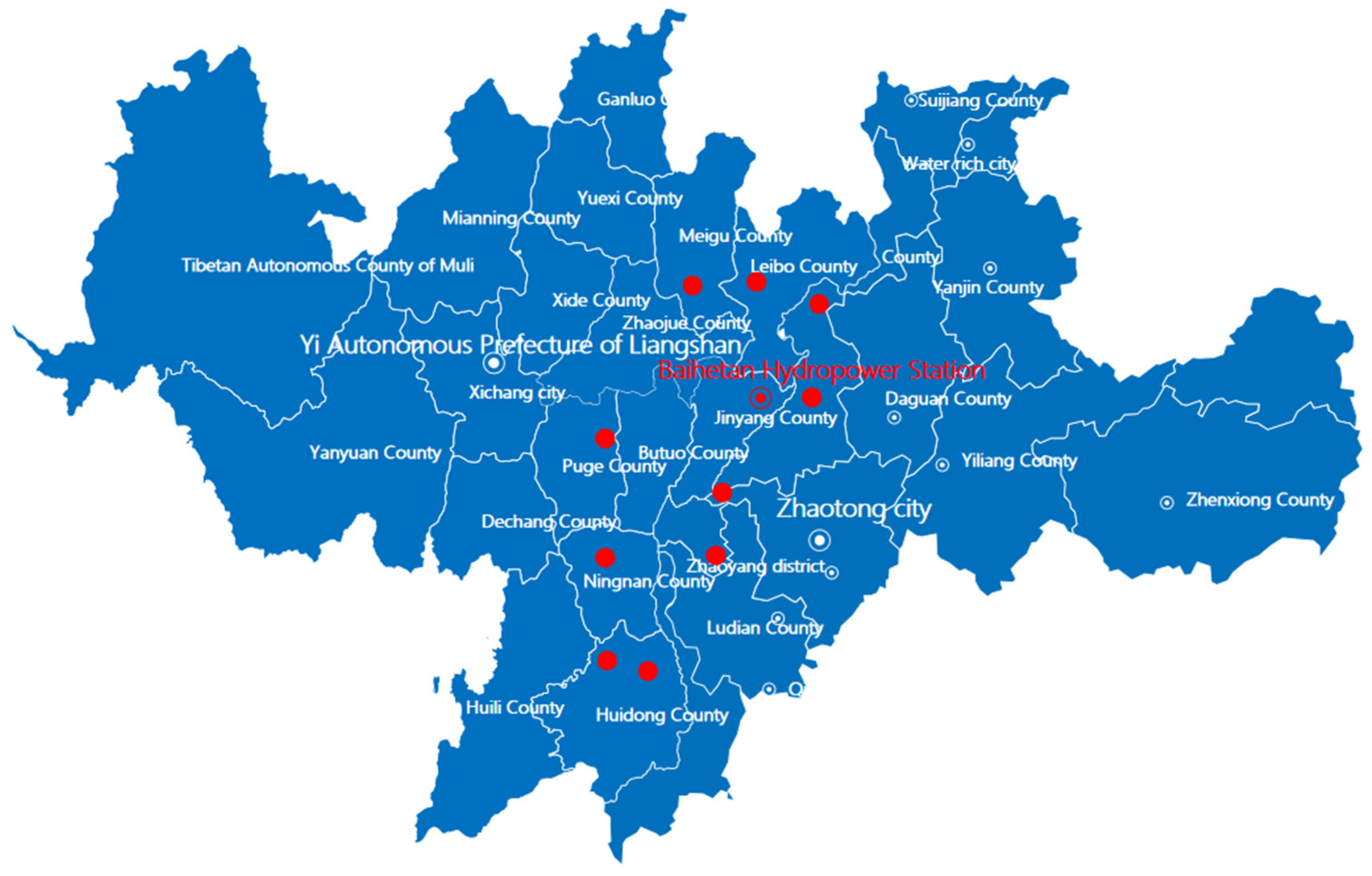
This paper takes the dam area of Baihetan Hydropower Station as the study area. Baihetan Hydropower Station is located at the junction of Dazhai Town, Qiaojia County, Yunnan Province, China and Liucheng Town, Ningnan County, Liangshan Yi Autonomous Prefecture, Sichuan Province, China. It is 75 km from Ningnan County. Baihetan Hydropower Station is the second of the four hydropower steps in the lower reaches of Jinsha River—Wudongde, Baihetan, Xiluodu and Xiangjiaba (Figure 1), about 41 km upstream from Qiaojia County and 182 km from Wudongde Dam Site; about 195 km downstream from Xiluodu Hydropower Station and about 380 km from Yibin City river mileage. The dam site controls a watershed area of 430,300 square km, accounting for 91% of the watershed area above the Jinsha River.
The ground meteorological data used are from 10 meteorological monitoring stations distributed in the area. The meteorological data in the area, including air pressure, air temperature and wind speed, are collected by hour.
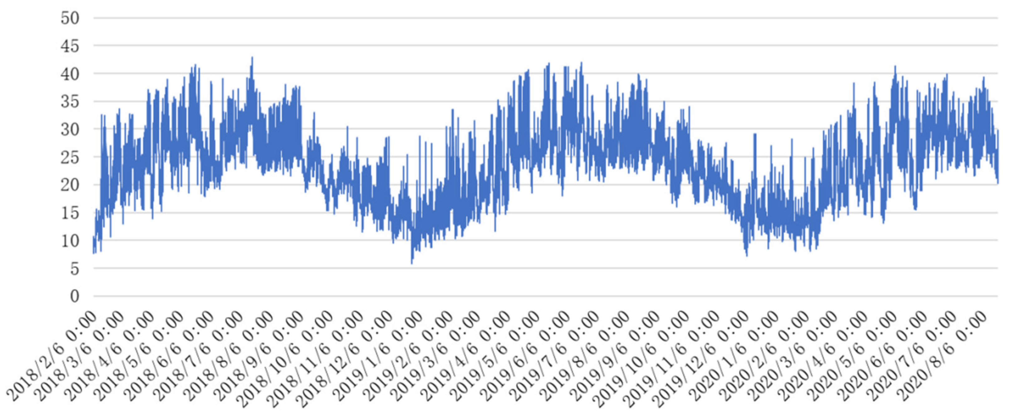
The air temperature dataset was obtained from 10 meteorological monitoring stations within the study area for a total of approximately 30 months of hourly air temperature observations from 2018 to 2020, including hourly mean air temperature, minimum air temperature, maximum air temperature, average air temperature, location (longitude and latitude) and time stamp for a total of 220,429 entries. Some sample data are shown in Table 1.
Figure 2 shows the variation of the hourly mean air temperature across the study area during the study period, with the lowest occurring in winter (29 December 2018 19:00), while the highest level was obtained in summer (18 July 2018 18:00).
2.2. Spatiotemporal Information Processing Module
The purpose of air temperature forecasting is to use air temperature change data from past time periods to forecast air temperature changes in future time periods. The air temperature monitoring stations in the region are distributed in the form of points. The monitoring data of individual stations represent the air temperature conditions at the locations of the stations. Previous studies have focused on the prediction of a single location, but in order to predict the air temperature change of the whole region at the same time, this paper first gridded the whole region, and then the point distribution of the monitoring station is mapped into a graph series by a spatial interpolation algorithm. In this way, we can use the historical graph series to predict the future graph series, thus achieving the regional temperature prediction task. First, the spatiotemporal information processing module proposed in this paper is introduced.
2.2.1. Regional Gridding
Traditionally, air temperature prediction methods are oriented toward a single location, which makes it difficult to solve the demand for regional air temperature prediction. In reality, weather monitoring stations are distributed in various locations in the region. In this paper, we first use GIS technology to vectorize the region to obtain a regional vector map and to project all weather monitoring stations to the corresponding locations in the regional vector map based on geographic coordinates. Then, grid the whole region and assign the information of all stations to the corresponding grids. The spatiotemporal map is defined to map the monitoring data of all stations into a unified spatiotemporal feature space. Finally, the single location-oriented prediction form is converted into a region-oriented spatiotemporal sequence prediction form.
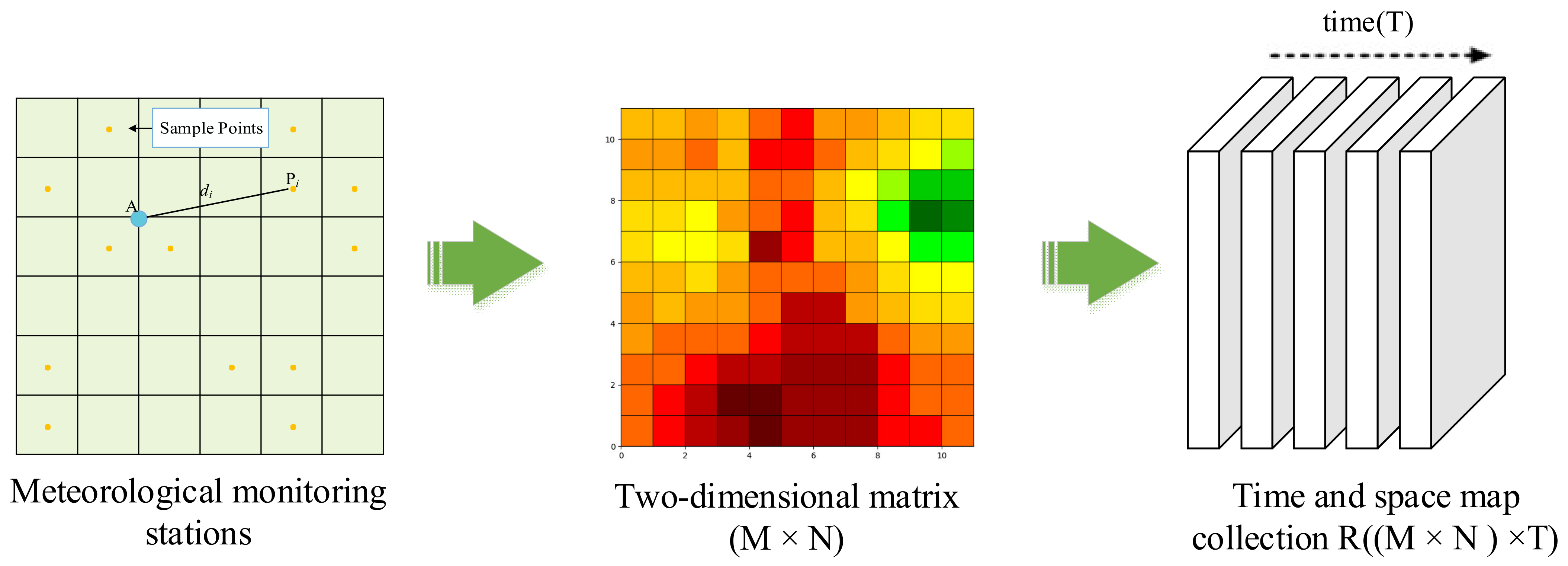
The distribution of each meteorological monitoring station in the region is distributed as a point distribution. This point distribution needs to be converted into a graphical form to represent the global distribution of air temperature in space. After obtaining the regional vector map using GIS technology, we divided the map into M × N girds according to the area size and the number of stations. We obtained 11 × 11 grids of size 500 m × 500 m. For each monitoring station and its monitoring value, we correspond to the grid in the map according to its latitude and longitude. For those grids corresponding to multiple stations, the average of multiple stations is taken as the final allocation to the grid.
For a regional grid map, it represents the air temperature distribution of the whole region at a given time t, which is defined as a two-dimensional matrix of size M × N. For consecutive time nodes T = (t1, …, t2, …, tn), the air temperature of the whole region changes over time. Therefore, the combination of graphs in the time nodes T can represent the spatial-temporal changes of air temperature in the whole region, which is defined as the collection R with the size of (M × N) × T. Figure 3 shows the overall process of constructing the spatiotemporal graph series.
2.2.2. Spatial Data Interpolation
For blank grids where air temperature monitoring values do not exist in the figure, they need to be data-populated using existing data to represent the approximate distribution of air temperature in space in this region, which is necessary for the subsequent use of deep spatiotemporal networks to capture the complete spatial variation process of temperature. Here, we use a spatial interpolation model to convert the existing air temperature monitoring values at the station to the actual observations approximated by these grids (for blank grids that are not in the region range, no interpolation is done to fill in with zeros), for which our core assumption is that, for any given grid, its air temperature is spatially closely related to its neighboring regions.
2.2.3. Classification of Spatial Interpolation Algorithms
Depending on the number of reference points used for estimation, the existing spatial data interpolation methods can be divided into global and local fitting methods, where the former uses the values of all existing reference points to estimate the value of the interpolation point, while the latter uses the partial values of the adjacent sample points to estimate the value of the interpolation point. In addition, existing interpolation methods for spatial data can be divided into exact and inexact interpolation methods. For interpolation points with known values, the exact interpolation method interpolates the same value at that point as the actual value at that point, while the inexact interpolation method does not guarantee the same. The spatial interpolation methods can also be divided into deterministic and stochastic according to whether the interpolation algorithm itself provides an error-checking model. Based on the above theory, the existing interpolation algorithms are classified and summarized in this paper, as shown in Table 2.
2.2.4. Principle of Inverse Distance Weight Interpolation
In this paper, we take the Inverse Distance Weight as an example here to illustrate the process of spatial data interpolation. Inverse Distance Weight interpolation, namely IDW, can also be called the distance inverse multiplication method. This means that the distance inverse multiplication square grid method is a weighted average interpolation method that can be interpolated in an exact or rounded way. The square parameter controls how the weight coefficient decreases with increasing distance from a gridded node. For a larger square, the closer data points are given a higher share of the weights, and for a smaller square, the weights are distributed more evenly across the data points.
IDW interpolation explicitly verifies the assumption that things that are closer to each other are more similar than things that are farther away from each other. When predicting values for any unmeasured location, the inverse distance weighting method uses measurements around the predicted location. The measurements closest to the predicted location have a greater influence on the predicted value than the measurements farther away from the predicted location. The inverse distance weighting method assumes that each measurement has a local influence that decreases with distance. Since this method assigns a larger weight to the point closest to the predicted location, while the weight decreases as a function of distance, it is called inverse Distance Weight. IDW follows the first law of geography that everything is related to everything else, but nearer things are more related than far things, and because of the use of weights, its interpolation for regional ranges does not produce incomprehensible or uninterpretable interpolation results. Its algorithm is defined as shown in Equation (1).
where Z is the interpolation result of the target grid, m is the number of sample points, and Zi is the ith (i = 1, 2, …, m) actual values of the sample points, n is the weight of the distance, and di is the distance from the ith sample point to the target grid, which is calculated as shown in Equation (2).
where xi, yi are the spatial coordinates of the i sample point, xA, yA are the spatial coordinates of the target grid.
2.2.5. Inverse Distance Weight Interpolation Process
Since things that are close to each other are more similar than things that are far away from each other, the relationship between the measured values and the predicted values will become less and less close as the distance between locations increases. To shorten the computation time, distant data points that have little impact on the prediction can be excluded (black points). Therefore, it is a common method to limit the number of measurements by specifying the search neighborhood. The shape of the neighborhood limits the search distance and the search location of the measurements to be used in the prediction. Other neighborhood parameters limit the locations that will be used in the shape. As shown in Figure 4, the orange circle has adjacent points, five measurement points (adjacent points, such as red points) are used when predicting values for locations with no measurements (orange points).
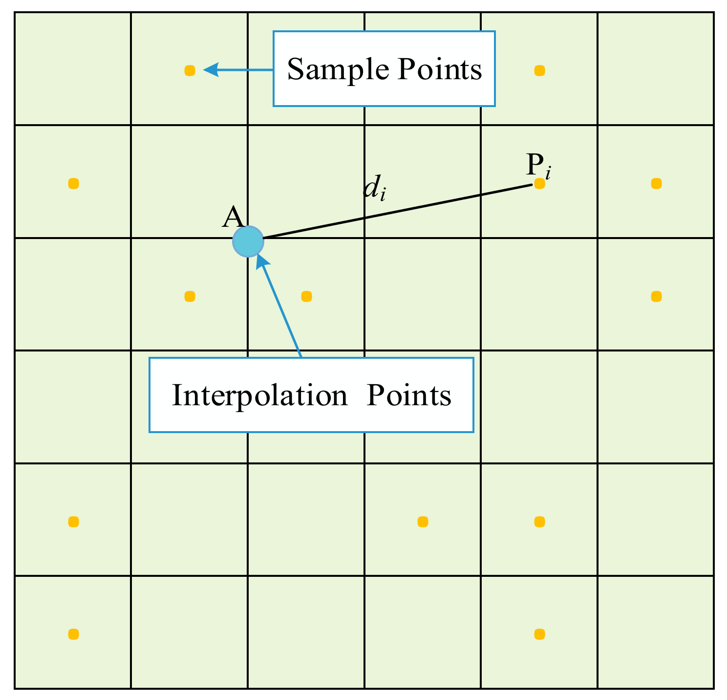
The blue point A is the interpolation point, and the other points are the sample points. Suppose there are a number of sample points within the fixed search radius of interpolation point A. For the interpolation point and the sample points, their own corresponding X, Y matrix coordinates on the grid matrix, as shown in the example in Figure 5.
Based on the principle of the IDW algorithm, the execution steps of IDW grid interpolation in this paper are as follows.
- (1)
- Input the values of all sample points and the grid matrix coordinates (X, Y) where they are located.
- (2)
- Determine the grid matrix coordinates of interpolation point A.
- (3)
- Determine the maximum search radius and the maximum number of sample points.
- (4)
- Search for the sample point Pi within the search radius. The distance di between the ith sample point Pi and interpolation point A is calculated according to Equation (2).
- (5)
- Calculates the estimated value Z of interpolation point A according to Equation (1).
- (6)
- Repeat steps (2), (3), (4), and (5) to find the values of all interpolated points.
2.3. Deep Spatiotemporal Prediction Module
2.3.1. Deep Spatiotemporal Prediction Model
The purpose of regional air temperature prediction is to input the historical air temperature graph series Xk (k = 0, 1, …, t − 1) to predict the future time air temperature graph series Xt, which represents the regional scale air temperature prediction results. At the same time, in reality, people are not only concerned about how the air temperature changes at a single time point in the recent future but also about the air temperature conditions at multiple time points in the future, which requires the construction of a model with a multi-step spatiotemporal prediction capability to effectively extract the spatiotemporal information and produce prediction results for multiple future time points. In this paper, a model design study is carried out based on deep learning technology. A deep spatiotemporal network prediction model is constructed to capture the complex nonlinear spatiotemporal information in the air temperature graph series to obtain the final short-term air temperature multi-step prediction results.
2.3.2. Long Short-Term Memory
Long Short-Term Memory (LSTM) is a recurrent neural network that solves the gradient explosion problem of traditional recurrent neural networks. Hua and Zhao et al. [33] proposed deep learning with long short-term memory for time series prediction. It solves the long-term dependence problem and reduces computational costs. Due to its unique structure, it is widely used to predict events with long intervals and time delays in time series. LSTM introduces the concept of “gates” to selectively let information pass through, which include forgetting gates, input gates and output gates. The LSTM unit has three inputs at time t, the input value xt of the network at the current moment, the output value ht − 1 of the unit at the previous moment, and the state ct − 1 of the unit at the previous moment. The LSTM unit has two outputs at time t, the output value ht at the current moment, and the state ct of the unit at the current moment. The forward propagation process of the LSTM network to process the input xt and finally generate the output ht can be divided into six steps, as follows.
Equations (3)–(8) distributions calculate the forgetting gate ft, the input gate it, the new information ct of the writing unit, the output gate ot, and the short-time output vector ht of the unit. Where Wif, Wii, Wic, and Wio distributions are the weight matrices of the current input multiplied by the forgetting gate, the input gate, the new information ct of the writing unit, and the output gate, respectively. Wfh, Wih, Wch, and Who are the weight matrices of the last output multiplied by the forgetting gate, the input gate, the new information of the writing unit, and the output gate, respectively. bf, bi, bc, and bo are the corresponding bias terms, and σ is the sigmoid function.
The main drawback of LSTM processing spatiotemporal data is that the input one-dimensional vector must be expanded before processing. Thus, all spatial information is lost during processing. Therefore, it is difficult for the traditional LSTM network to solve the spatiotemporal prediction problem of regional temperature.
2.3.3. Convolutional Long Short-Term Memory
Convolutional Long Short-Term Memory (ConvLSTM) is an extension of the currently popular Long Short-Term Memory (LSTM) network, with the goal of overcoming the shortcomings of LSTM when dealing with spatiotemporal data. Specifically, in the ConvLSTM network, the fully connected gates of the LSTM module are replaced by convolutional gates to encode spatiotemporal features. Following the conventional representation, let Xt, Ht, ct and yt denote the input, hidden state, cell state and output of the ConvLSTM network at moment t, respectively. The equations describing the ConvLSTM are as follows.
where, W and b are trainable parameters whose sizes match the corresponding tensor. All gate activations and hidden states in ConvLSTM are three-dimensional tensors that can handle both temporal and spatial information. The vectors in the traditional LSTM lose natural spatial information and can only handle the temporal dimension. Therefore, this paper is based on ConvLSTM to construct a prediction model of regional temperature.
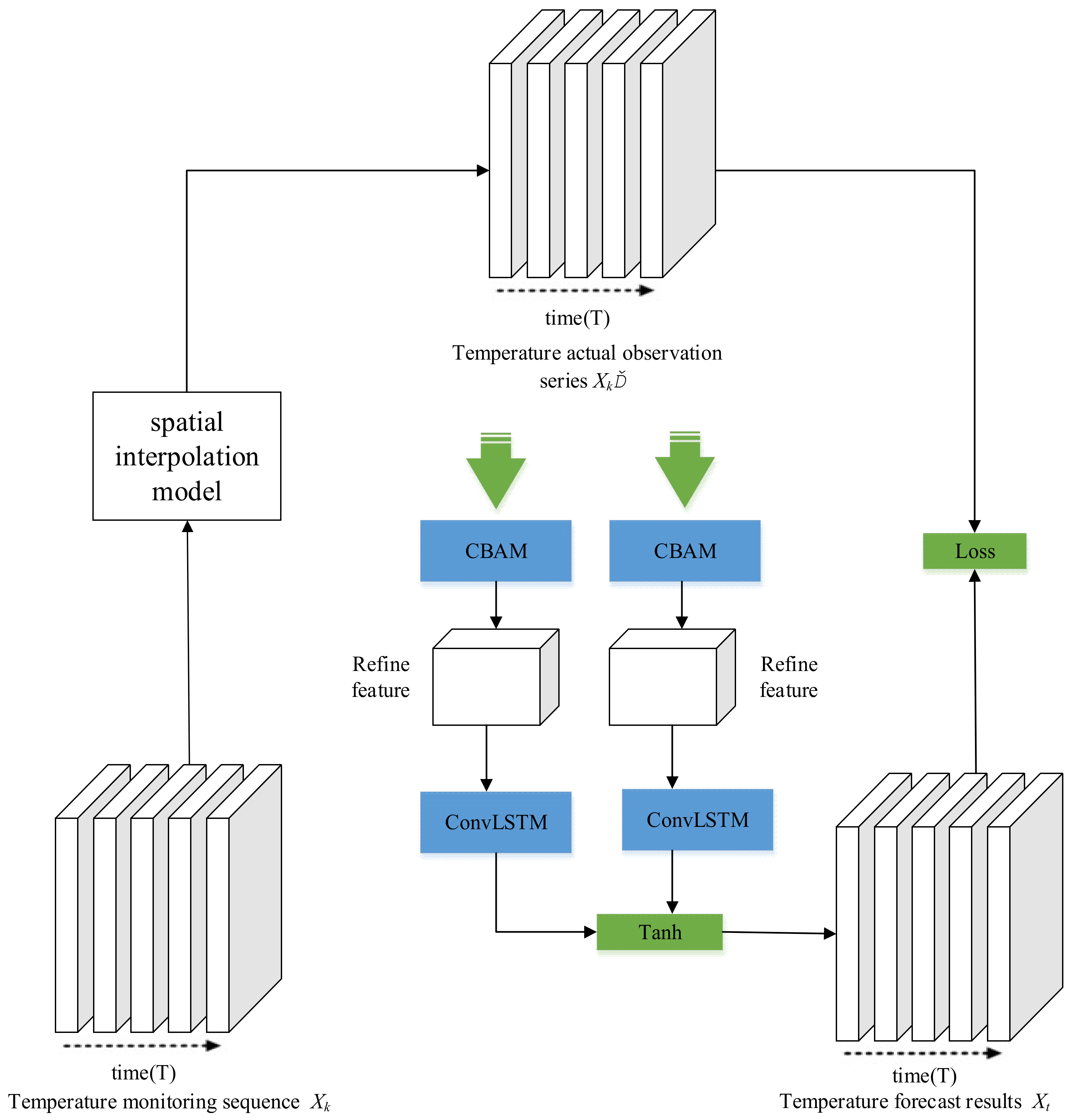
2.3.4. Model Structure
ConvLSTM is a structure that combines CNN and LSTM, which uses CNN to capture spatial features in multidimensional data and uses LSTM for time-series prediction modeling. Therefore, ConvLSTM can not only extract spatial features but also temporal features. In this paper, a deep spatiotemporal network model, ST-Net, is designed for regional air temperature prediction based on the ConvLSTM structure. The attention mechanism module CBAM (Convolutional Block Attention Module) is added to improve the prediction capability of the model for extreme air temperature cases. The model structure of ST-Net is shown in Figure 6.
2.3.5. Attention Module CBAM
An important property of the human visual system is that people do not try to process the entire scene they see at the same time. Instead, to better capture visual structure, humans use a series of local glimpses that selectively focus on salient parts. In recent years, there have been attempts to introduce attention mechanisms into convolutional neural networks to focus on salient parts of an image to improve their performance in computer vision tasks.
Corresponding to the task of spatiotemporal prediction of regional temperatures, the attention mechanism can be used to better capture extreme variations in regional temperatures. Such as low or high temperatures, especially for extreme high temperatures, which is important to guide realistic production activities. In this paper, the attention mechanism is introduced into the prediction model to forecast extreme temperatures more effectively.
2.3.6. Overall Structure of CBAM
The Convolutional Block Attention Module (CBAM) is a lightweight module that combines channel attention and spatial attention, which, like SENet, can be embedded in almost any CNN network to dramatically improve model performance while bringing a small amount of computation and a number of parameters. The overall structure of the CBAM module is shown in Figure 7.
2.3.7. Channel Attention
Channel attention focuses on “what” is meaningful to the input image. Its principle structure is shown in Figure 8. In order to efficiently compute channel attention, the spatial dimension of the input feature map needs to be compressed. For the aggregation of spatial information, the common method is average pooling. However, it has been suggested that maximum pooling collects another important clue about unique object features that can infer attention on finer channels. Therefore, the average pooling and maximum pooling features are used simultaneously.
Fcavg and Fcmax in Equation (14) denote the average pooling feature and the maximum pooling feature, respectively. These two descriptors are then forwarded to a shared network to produce our channel attention graph Mc. The shared network consists of a multilayer perceptron (MLP) with an implicit layer. To reduce the parameter overhead, the activation size of the hidden layer is set to R/C = r × 1 × 1, where R is the descent rate. After applying the shared network to each descriptor, the output feature vectors are combined using element-wise summation. σ denotes the sigmoid function. Mc(F) is element-wise multiplied by F to obtain F′.
Compared to SE-Net, which only uses a global-level pooling layer to compress channel features. Maximum pooling can collect more important cues between indistinguishable objects to obtain more detailed channel attention. Therefore, CBAM uses both the average pooled and maximum pooled features and then feeds them sequentially into a weight-sharing multilayer perceptron (MLP). Finally, the respective output features are summed at corresponding positions.
2.3.8. Spatial Attention
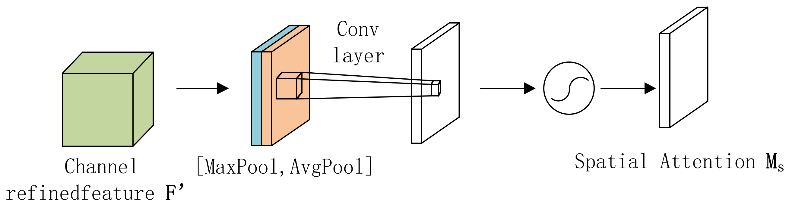
Spatial attention is focused on “where” is the most informative part, which complements channel attention. Its principle structure is shown in Figure 9. To compute spatial attention, average pooling and maximum pooling operations are applied along the channel axes, and then they are concatenated to generate a valid feature descriptor. A convolutional layer is then applied to generate a spatial attention map Ms(F) of size R × H × W, as shown in Equation (15), which encodes the locations that need attention or suppression.
Specifically, two pooling operations are used to aggregate the channel information of a feature map to generate two two-dimensional graphs, the size of the Fsavg is 1 × H × W. the size of the Fsmax is 1 × H × W. Among them, σ represents a sigmoid function, and f 7 × 7 denotes a convolution operation with a filter size of 7 × 7.
The inclusion of the spatial attention module compensates, to some extent, for the lack of channel-only attention. Spatial attention focuses mainly on which part of the input image is richer in valid information. It is worth noting that the pooling operation here is performed along the channel axis, comparing the values between different channels for each pooling instead of the values of different regions of the same channel. One feature map is obtained by maximum pooling and one by average pooling, and then they are stitched together into a 2-D feature map and then input into a standard 7 × 7 convolution for parameter learning. Finally, a 1-D weighted feature map is obtained.
3. Experimental Results and Visualization
3.1. Dataset Processing (Study Area and Dataset)
We experimented with an Ubuntu system (Groovy Gorilla 20.10) with 32G of RAM. The CPU version is IntelI XI(R) Gold 5218. The GPU version is NVIDIA RTX 6000. The Python version is 3.6. The PyTorch version is 1.8.1.
First, 30 months of air temperature observations were transformed into 22,240 maps using the spatiotemporal information processing module, with the first 70% of the data serving as the training set and the last 30% as the test set. Next, the training and test sets were slide-cut using a window with a size of 12 h. As a result, a total of 22,218 sequences were generated, each containing 12 graphs (6 for input and 6 for prediction). Finally, 15,553 graph sequences were obtained for training and 6665 graph sequences were used for testing.
The number of network lIyers is 4. The convolution kernel size of the model used is 3 × 3. The maximum Epoch is set to 150. The Batch size is set to 16. The learning rate is set to 0.001, and the optimizer is Adam. In order to prevent the over-fitting of training data in the process of model training, the original training set was divided into the training set and the verification set according to the ratio of 7:3. The early stop method [34] was adopted to assist the training process. When the error of the model on the verification set was worse than the last training result, the training was stopped and the last iteration result was used as the final parameter of the model.
3.2. Evaluation Metrics
We uses three metrics to evaluate the performance of air temperature prediction. Mean absolute error (MAE), Root mean square error (RMSE), and Coefficient of determination (R2) are used to evaluate the error and stability between the predicted value and the real value yt+h,i at time point i. is the sample mean. N is the number of samples in the test set. Their formula is defined as follows:
Mean absolute error (MAE):
Root mean squared error (RMSE):
Coefficient of determination (R2):
3.3. Prediction Performance Comparison
3.3.1. Single-Step Duration Prediction
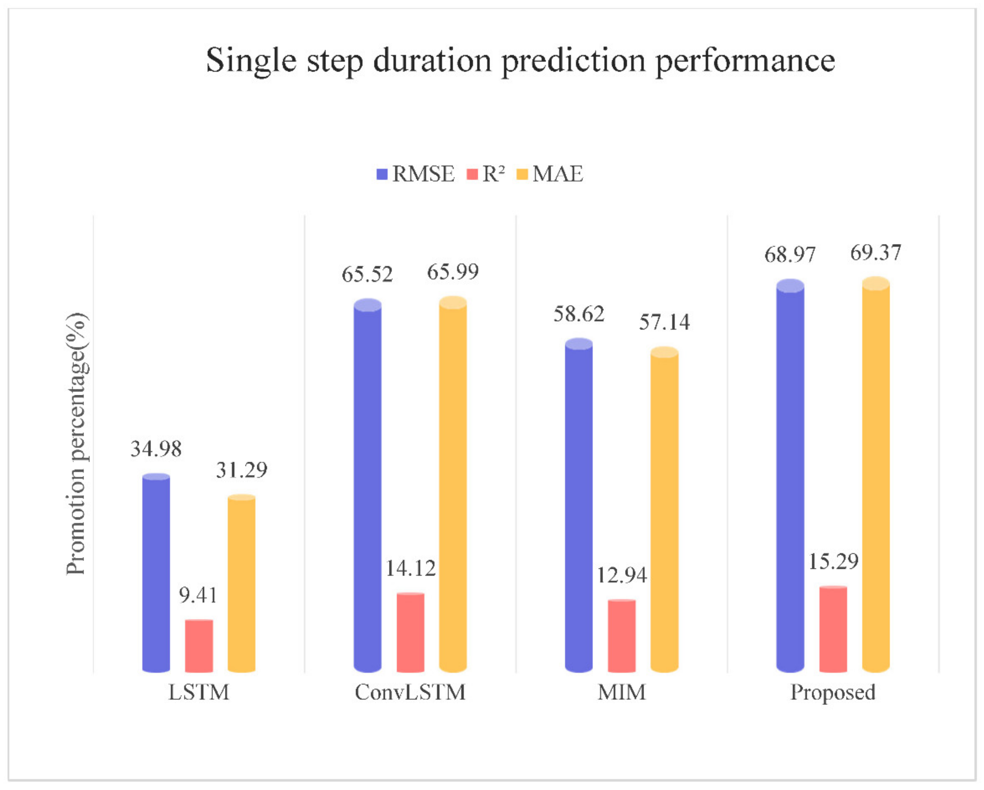
This section shows the single-step temporal prediction performance comparison, i.e., the prediction of the future 1-h air temperature change using historical air temperature monitoring data. Table 3 shows the prediction performance of the model proposed in this paper on the test set and compares it with the current mainstream spatiotemporal prediction model ConvLSTM, Memory in Memory (MIM), which is compared with two spatiotemporal prediction models in detail. The ST-Net proposed in this paper has superior performance compared with MIM. As shown in Figure 10, the RMSE, R2 and MAE of ST-Net changed 68.97%, 15.29% and 69.37% respectively compared to CNN. The experimental results of MIM changed less than that of ST-Net. Notably, the model parameter of ST-Net is 63% of ConvLSTM and 29% of MIM, which means a lower memory demand. Meanwhile, the training time consumption of ST-Net is only 40% of MIM and prediction time consumption is only 47% of MIM. Therefore, ST-Net is better suited for realistic model deployment.
3.3.2. Multi-Step Duration Prediction
Furthermore, we used historical observations to predict the regional air temperature change at the next 6 h. The prediction performance of these models is compared, as shown in Table 4. With the increase in the time step, the performance of these models decreases. However, the proposed model always shows the best performance. The prediction performance of the ConvLSTM model in the first 2 h is higher than that of the MIM, indicating that the MIM model improves the prediction ability for long-term data compared to the ConvLSTM model but decreases the prediction performance for the most recent time point. It is noteworthy that the prediction performance of ST-Net is consistently better than that of ConvLSTM and MIM in the time span of 6 h, which demonstrates that the proposed model can better learn the spatial and temporal changes in air temperature to obtain better prediction performance at multiple time steps.
3.3.3. Individual Site Predictions
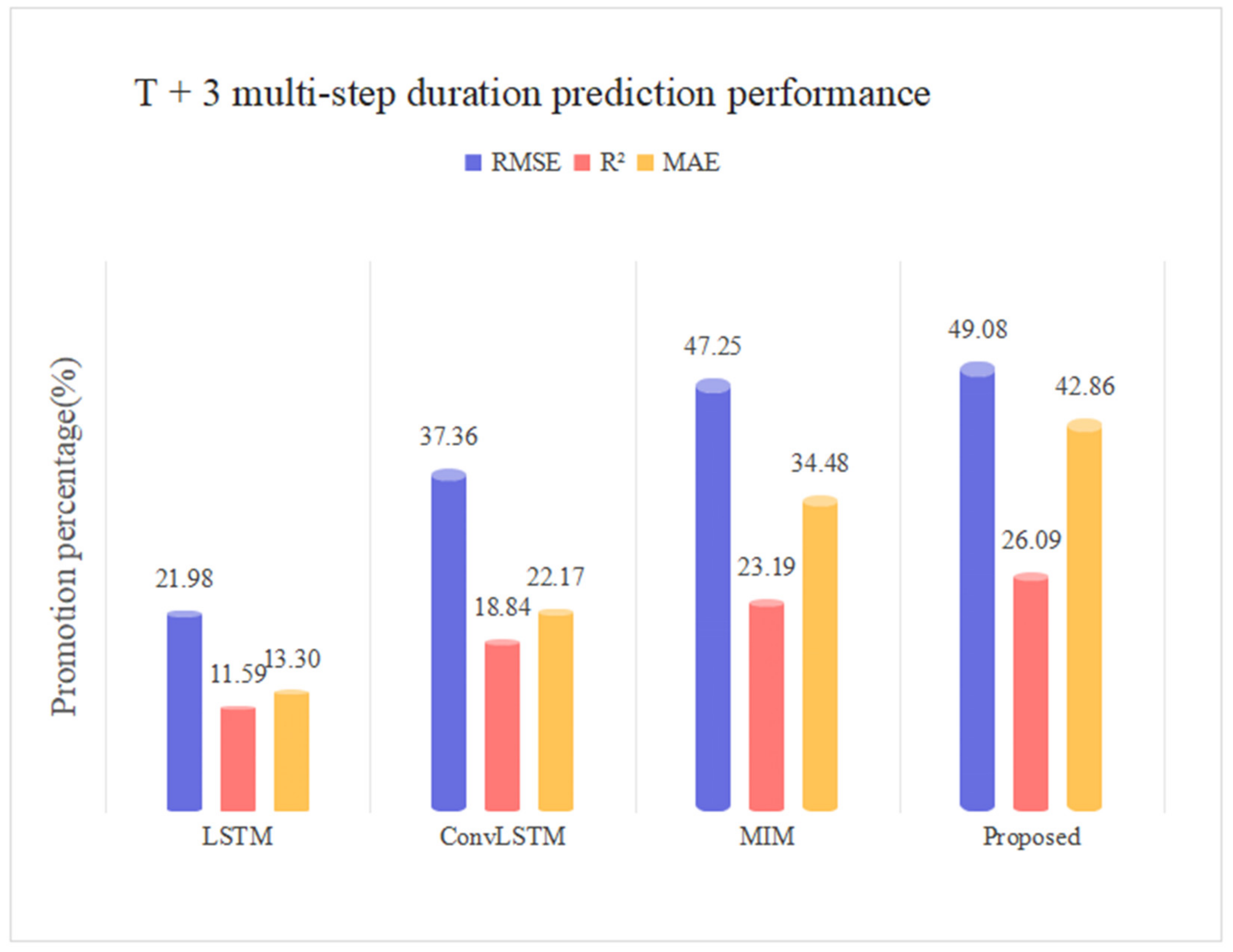
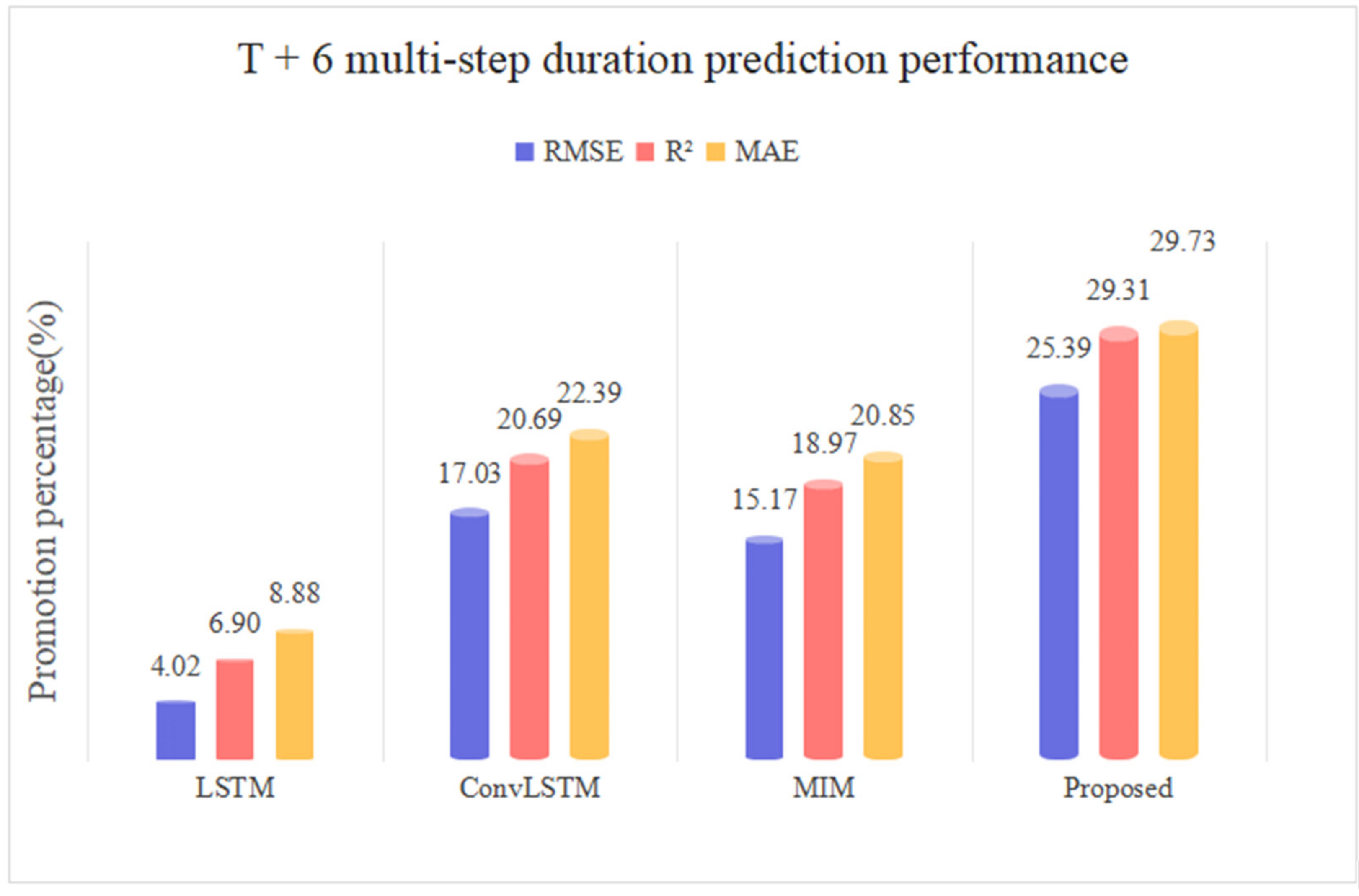
In addition to evaluating the regional air temperature prediction performance, this paper also tests the prediction capability of ST-Net for a single location and compares it with other models. Here, the prediction capability of a meteorological monitoring station for the next three and six moments is further analyzed and the results are shown in Table 4. As shown in Figure 11, the RMSE, R2 and MAE of ST-Net changed by 49.08%, 26.09% and 42.86% at the moment T + 3 compared to CNN, respectively. As shown in Figure 12, the RMSE, R2 and MAE of ST-Net changed by 25.39%, 29.31% and 29.73% respectively at T + 6, compared to CNN. From the prediction results for individual stations, ST-Net still shows the best prediction ability, while MIM is still weaker than ST-Net for the last three and six moments, which is consistent with the previous regional air temperature prediction results.
3.4. Visualization of Prediction Results
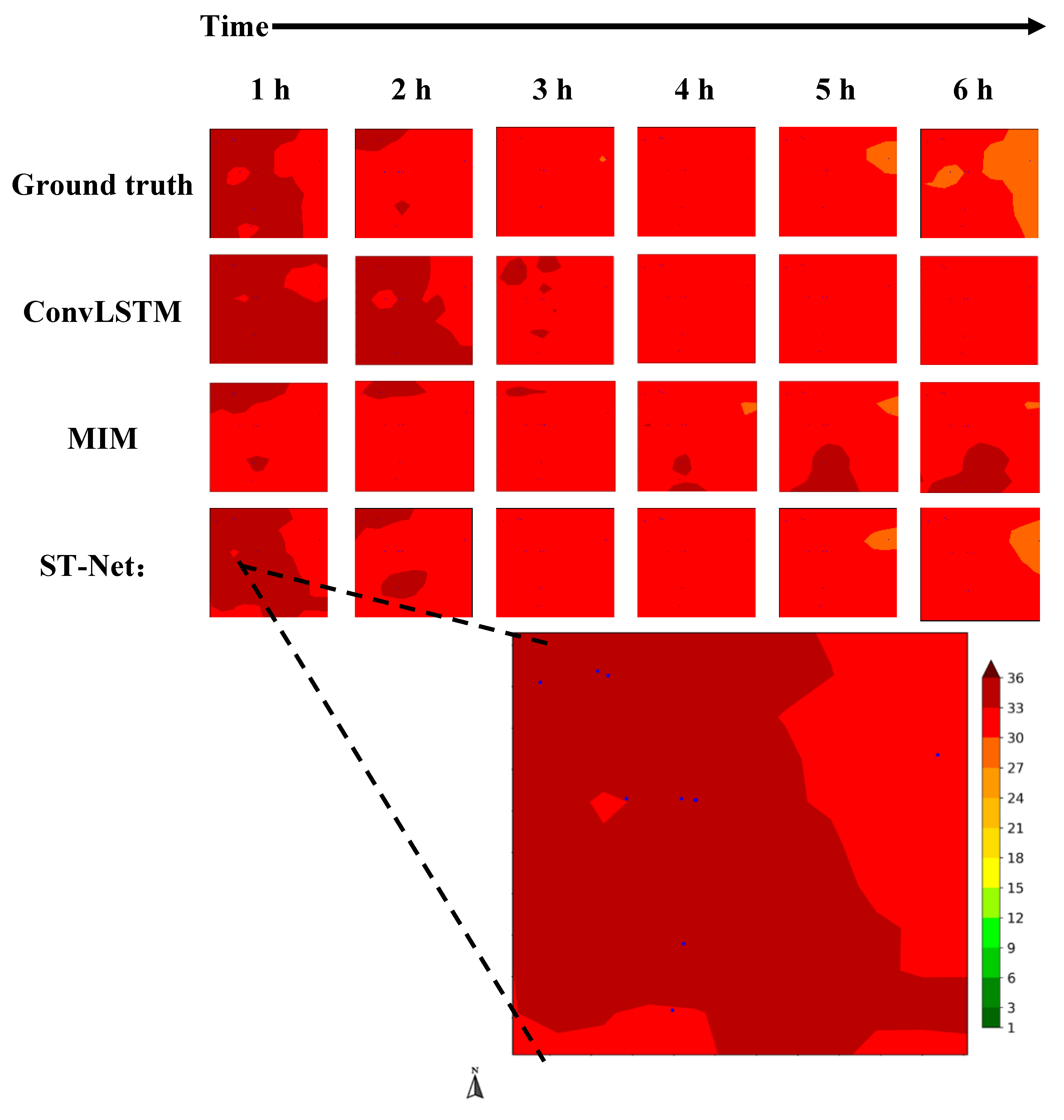
The purpose of regional air temperature prediction is to give the future air temperature conditions and the trend of changes at any location in the region, which can provide important decision support for realistic construction and personnel safety, project quality and safety, risk management and cost control. Figure 13 shows a 6-h sequence of regional air temperature prediction maps given by each method and compared with the real air temperature map sequence. It can be seen that the method proposed in this paper can well predict the high temperature in the western part of the study area in the first hour of the future and the trend of gradually decreasing air temperature in the next 5 h. ConvLSTM has some prediction ability for the regional air temperature in the next 1 h, while MIM has the weakest prediction ability relatively for the next 1 h, but the prediction ability of MIM for the regional air temperature with multi-step duration is stronger than ConvLSTM.
4. Discussion
Our proposed ST-Net achieves the best RMSE, R2 and MAE compared to other traditional models. ST-Net has the best predictions for the next 1 h compared to a longer time. This is also reflected in the visualized images of the prediction results, where ST-Net’s prediction images 1 h ahead are closer to the real temperature image than other methods. This reflects the superiority of the model proposed in this paper. In addition, ST-Net is more lightweight and has a shorter training time. However, our proposed model also has some limitations. Due to the small sample size of the dataset, the model is suitable for temperature prediction in a specific small area. In the future, we will investigate how to expand the dataset to enhance the generalization of the model.
5. Conclusions
In this paper, a deep spatiotemporal network-based air temperature prediction method is proposed for simultaneously predicting the air temperature variation of the whole region. The spatiotemporal information processing component is used to convert the point-distributed air temperature monitoring data into a spatiotemporal graph sequence, and then a deep learning model is used to learn the complex nonlinear spatiotemporal variations in the graph sequence and, finally, to obtain the short-term air temperature prediction results at the regional scale. Based on air temperature collection data from 10 meteorological monitoring stations at Baihetan Hydropower Station to implement short-term air temperature prediction. At the first hour of the future, the RMSE, R2 and MAE of ST-Net reached 0.63, 0.98, and 0.45, respectively. At the moment of T + 3, the RMSE, R2 and MAE of ST-Net reached 1.39, 0.87, and 1.16, respectively, and at the moment of T + 6, the RMSE, R2 and MAE of ST-Net reached 2.41, 0.75, 1.82 and 1.82, respectively. Our proposed method can predict air temperature changes on a regional scale and thus provide important decision support for realistic engineering management.
Author Contributions
Conceptualization and Validation, S.W.; Formal analysis, Writing—original draft, and Methodology, F.F.; Writing—review & editing, F.F. and M.Y.; Data curation and Funding acquisition, L.W.; Validation, S.D.; Data processing, Y.H.; Formal analysis, Q.Z.; Software design, R.G. All authors have read and agreed to the published version of the manuscript.
Funding
This research was funded by the research and application of key meteorological forecasting techniques for hydropower stations in the lower reaches of Jinsha River, grant number JG/20015B, the Shanghai science and technology innovation action plan special project of artificial intelligence science and technology support, grant number 20511101600, “Research on solar radiation identification and prediction model based on artificial intelligence and image”, grant number “2022XXJ-5”, and Shaanxi Meteorological Information Center unveiled the list of scientific and technological projects.
Informed Consent Statement
Informed consent was obtained from all subjects involved in the study.
Data Availability Statement
The data presented in this study are available on request from the corresponding author. The data are not publicly available due to the atmospheric temperature data is real station data and contains location information.
Conflicts of Interest
The authors declare no conflict of interest.
References
- Tian, D.; Wei, X.; Wang, Y.; Zhao, A.; Mu, M.; Feng, J. Prediction of temperature in edible fungi greenhouse based on MA-ARIMA-GASVR. Trans. Chin. Soc. Agric. Eng. 2020, 36, 190–197. [Google Scholar]
- Xie, Q.; Zheng, P.; Bao, J.; Su, Z. Thermal Environment Prediction and Validation Based on Deep Learning Algorithm in Closed Pig House. J. Agric. Mach. 2020, 51, 353–361. [Google Scholar]
- Li, F.; Zeng, X.; Wei, M.; Ding, M. Short-term wind power forecasting based on cluster analysis and a hybrid evolutionary-adaptive methodology. Power Syst. Prot. Control 2020, 48, 151–158. [Google Scholar]
- Meng, X.; Wang, R.; Zhang, X.; Wang, M.; Qiu, G.; Wang, Z. Ultra-short-term wind power prediction based on empirical mode decomposition and multi-branch neural network. J. Comput. Appl. 2021, 41, 237–242. [Google Scholar]
- Han, Y.; Mi, L.; Shen, L.; Cai, C.S.; Liu, Y.; Li, K. A short-term wind speed interval prediction method based on WRF simulation and multivariate line regression for deep learning algorithms. Energy Convers. Manag. 2022, 258, 115540. [Google Scholar] [CrossRef]
- Chen, Y.; Wang, Y.; Dong, Z.; Su, J.; Han, Z.; Zhou, D.; Zhao, Y.; Bao, Y. 2-D regional short-term wind speed forecast based on CNN-LSTM deep learning model. Energy Convers. Manag. 2021, 244, 114451. [Google Scholar] [CrossRef]
- Ji, L.; Fu, C.; Ju, Z.; Shi, Y.; Wu, S.; Tao, L. Short-Term Canyon Wind Speed Prediction Based on CNN—GRU Transfer Learning. Atmosphere 2022, 13, 813. [Google Scholar] [CrossRef]
- Yang, D.; Li, J.; Lv, J.; Yang, W.; Wang, X. Research on solar direct normal irradiance prediction model based on improved CNN for concentrating solar power station. Renew. Energy Resour. 2021, 39, 182–188. [Google Scholar]
- Zhang, Q.; Fu, F.; Tian, R. A deep learning and image-based model for air quality estimation. Sci. Total Environ. 2020, 724, 138178. [Google Scholar] [CrossRef] [PubMed]
- Zhang, Q.; Gao, T.; Liu, X.; Zheng, Y. Exploring the influencing factors of public environmental satisfaction based on socially aware computing. J. Clean. Prod. 2020, 266, 121774. [Google Scholar] [CrossRef]
- Cobaner, M.; Citakoglu, H.; Kisi, O.; Haktanir, T. Estimation of mean monthly air temperatures in Turkey. Comput. Electron. Agric. 2014, 109, 71–79. [Google Scholar] [CrossRef]
- Ozbek, A.; Sekertekin, A.; Bilgili, M.; Arslan, N. Prediction of 10-min, hourly, and daily atmospheric air temperature: Comparison of LSTM, ANFIS-FCM, and ARMA. Arab. J. Geosci. 2021, 14, 622. [Google Scholar] [CrossRef]
- Cheng, Z.; Zhuang, L.; Zhang, Y.; Wu, M.; Li, X.; Zhao, Y. Improvement of the Format and Transmission Mode of the Uploaded Data File in the Agrometeorological Observing Data Operation System. Chin. J. Agrometeorol. 2021, 42, 243–249. [Google Scholar]
- Hou, Y.; Zhang, L.; Wu, M.; Song, Y.; Guo, A.; Zhao, X. Advances of Modern Agrometeorological Service and Technology in China. J. Appl. Meteorol. Sci. 2018, 29, 641–656. [Google Scholar]
- Xiong, M. Calibrating daily 2 m maximum and minimum air temperature forecasts in the ensemble prediction system. Acta Meteorol. Sin. 2017, 75, 211–222. [Google Scholar]
- Pérez-Lombard, L.; Ortiz, J.; Pout, C. A review on buildings energy consumption information. Energ Build. 2008, 40, 394–398. [Google Scholar] [CrossRef]
- Qu, Z.; Shang, X.; Wang, J.; Liang, Y.; Gao, F.; Yang, F. Vertical temperature distribution and its forecast for two tree structures of apple orchard during the blooming period in the Loess Plateau. Chin. J. Appl. Ecol. 2015, 26, 3405–3412. [Google Scholar]
- Duan, W.; Wang, Y.; HUo, Z.; Zhou, F. Ensemble forecast methods for numerical weather forecast and climate prediction: Thinking and prospect. Clim. Environ. Res. 2019, 24, 396–406. [Google Scholar]
- Frnda, J.; Durica, M.; Nedoma, J.; Zabka, S.; Martinek, R.; Kostelansky, M. A weather forecast model accuracy analysis and ecmwf enhancement proposal by neural network. Sensors 2019, 19, 5144. [Google Scholar] [CrossRef] [Green Version]
- Zhao, C.; Liu, D.; Xie, X.; Liu, J. Research on Seasonal Temperature Forecasting Based on Time Series. J. Anhui Jianzhu Univ. 2022, 30, 83–89. [Google Scholar]
- Hinke, T.H.; Rushing, J.; Ranganath, H.; Graves, S.J. Techniques and experience in mining remotely sensed satellite data. Artif. Intell. Rev. 2000, 14, 503–531. [Google Scholar] [CrossRef]
- Wabf, F.; Yuan, H.; Song, J.; Wang, Y. Research on precipitation forecasts in Nanjing City. J. Nanjing Univ. (Nat. Sci.) 2012, 48, 513–525. [Google Scholar] [CrossRef]
- Dimri, T.; Ahmad, S.; Sharif, M. Time series analysis of climate variables using seasonal ARIMA approach. J. Earth Syst. Sci. 2020, 129, 149. [Google Scholar] [CrossRef]
- Tan, X. The Application of the Method of Time Series Analysis in the Study of Chongqing Temperatures; College of Mathematics and Statistics of Chongqing University: Chongqing, China, 2016. [Google Scholar]
- Ismail Fawaz, H.; Forestier, G.; Weber, J.; Idoumghar, L.; Muller, P. Deep learning for time series classification: A review. Data Min. Knowl. Discov. 2019, 33, 917–963. [Google Scholar] [CrossRef] [Green Version]
- Tao, Y.; Du, J. Temperature prediction using long short term memorynetwork based on random forest. Comput. Eng. Des. 2019, 40, 737–743. [Google Scholar] [CrossRef]
- Mathew, A.; Sreekumar, S.; Khandelwal, S.; Kaul, N.; Kumar, R. Prediction of land-surface temperatures of Jaipur city using linear time series model. IEEE J. Sel. Top. Appl. Earth Obs. Remote Sens. 2016, 9, 3546–3552. [Google Scholar] [CrossRef]
- Wei, L.; Guan, L.; Qu, L. Prediction of sea surface temperature in the South China Sea by artificial neural networks. IEEE Geosci. Remote Sens. Lett. 2019, 17, 558–562. [Google Scholar] [CrossRef]
- Dong, D.; Sheng, Z.; Yang, T. Wind power prediction based on recurrent neural network with long short-term memory units. In Proceedings of the 2018 International Conference on Renewable Energy and Power Engineering (REPE), Toronto, ON, Canada, 24–26 November 2018; pp. 34–38. [Google Scholar]
- Xiaoyun, Q.; Xiaoning, K.; Chao, Z.; Shuai, J.; Xiuda, M. Short-term prediction of wind power based on deep long short-term memory. In Proceedings of the 2016 IEEE PES Asia-Pacific Power and Energy Engineering Conference (APPEEC), Xi’an, China, 25–28 October 2016; pp. 1148–1152. [Google Scholar]
- Dai, H.; Huang, G.; Zeng, H.; Zhou, F. PM2.5 volatility prediction by XGBoost-MLP based on GARCH models. J. Clean. Prod. 2022, 356, 131898. [Google Scholar] [CrossRef]
- Dai, H.; Huang, G.; Wang, J.; Zeng, H.; Zhou, F. Prediction of Air Pollutant Concentration Based on One-Dimensional Multi-Scale CNN-LSTM Considering Spatial-Temporal Characteristics: A Case Study of Xi’an, China. Atmosphere 2021, 12, 1626. [Google Scholar] [CrossRef]
- Hua, Y.; Zhao, Z.; Li, R.; Chen, X.; Liu, Z.; Zhang, H. Deep learning with long short-term memory for time series prediction. IEEE Commun. Mag. 2019, 57, 114–119. [Google Scholar] [CrossRef]
- Prechelt, L. Early stopping-but when? In Neural Networks: Tricks of the Trade; Springer: Berlin/Heidelberg, Germany, 1998; pp. 55–69. [Google Scholar]
Figure 1.
Geographical Location of Hydropower Station.

Figure 2.
Regional Average Air Temperature Change Chart.

Figure 3.
Spatiotemporal graph construction process.

Figure 4.
Diagram of the IDW search field.

Figure 5.
Schematic diagram of IDW interpolation.

Figure 6.
Structure of the ST-Net model.

Figure 7.
CBAM module structure.

Figure 8.
Channel Attention Structure.

Figure 9.
Spatial attention structure.

Figure 10.
Single-step duration prediction performance.

Figure 11.
T + 3 multi-step duration prediction performance.

Figure 12.
T + 6 multi-step duration prediction performance.

Figure 13.
Visualization images of regional air temperature (°C) forecast results.


Table 1.
Site Data Table.
| Datetime | Air Temperature (°C) | Wind Direction | Two-Wind Speed (m/s) | Two-Wind Direction | Humidity (% rh) | Pressure (pa) |
|---|---|---|---|---|---|---|
| 2018/6/2 1:00 | 24.5 | 345 | 4.8 | 340 | 43 | 965 |
| 2018/6/2 2:00 | 21.4 | 247 | 3.6 | 253 | 32 | 966 |
| 2018/6/2 3:00 | 20.3 | 350 | 6.5 | 356 | 36 | 965 |
| 2018/6/2 4:00 | 19.5 | 305 | 5.6 | 308 | 31 | 967 |
| 2018/6/2 5:00 | 20.1 | 334 | 6.2 | 336 | 31 | 966 |
| 2018/6/2 6:00 | 19.9 | 301 | 6.4 | 303 | 31 | 965 |
| 2018/6/2 7:00 | 19.8 | 298 | 5.6 | 295 | 33 | 965 |
| 2018/6/2 8:00 | 19.5 | 260 | 4.3 | 266 | 33 | 965 |
| 2018/6/2 9:00 | 19.7 | 192 | 4.1 | 196 | 32 | 965 |
| 2018/6/2 10:00 | 20.8 | 208 | 3.8 | 210 | 38 | 967 |
Table 2.
Classification of spatial data interpolation methods.
| Global Fitting Method | Local Fitting Method | ||
|---|---|---|---|
| deterministic | stochastic | deterministic | stochastic |
| Trend surface (non-exact) | Regression (non-exact) | Inverse distance weight (exact) | Kriging (exact) |
| Thiesen (exact) | |||
| Spline interpolation (exact) | |||
Publisher’s Note: MDPI stays neutral with regard to jurisdictional claims in published maps and institutional affiliations. |
© 2022 by the authors. Licensee MDPI, Basel, Switzerland. This article is an open access article distributed under the terms and conditions of the Creative Commons Attribution (CC BY) license (https://creativecommons.org/licenses/by/4.0/).
Share and Cite
MDPI and ACS Style
Wu, S.; Fu, F.; Wang, L.; Yang, M.; Dong, S.; He, Y.; Zhang, Q.; Guo, R. Short-Term Regional Temperature Prediction Based on Deep Spatial and Temporal Networks. Atmosphere 2022, 13, 1948. https://doi.org/10.3390/atmos13121948
AMA Style
Wu S, Fu F, Wang L, Yang M, Dong S, He Y, Zhang Q, Guo R. Short-Term Regional Temperature Prediction Based on Deep Spatial and Temporal Networks. Atmosphere. 2022; 13(12):1948. https://doi.org/10.3390/atmos13121948
Chicago/Turabian StyleWu, Shun, Fengchen Fu, Lei Wang, Minhang Yang, Shi Dong, Yongqing He, Qingqing Zhang, and Rong Guo. 2022. "Short-Term Regional Temperature Prediction Based on Deep Spatial and Temporal Networks" Atmosphere 13, no. 12: 1948. https://doi.org/10.3390/atmos13121948
Note that from the first issue of 2016, this journal uses article numbers instead of page numbers. See further details here.