
Exploring Non-Linear Dependencies in Atmospheric Data with Mutual Information
by
 , , , and
Petri Laarne
1,2 ,
,
Emil Amnell
1,
Martha Arbayani Zaidan
1,3,
Santtu Mikkonen
4,5 and
Tuomo Nieminen
1,6,* 1
Institute for Atmospheric and Earth System Research/Physics, Faculty of Science, University of Helsinki, P.O. Box 64, 00014 Helsinki, Finland
2
Department of Mathematics and Statistics, University of Helsinki, P.O. Box 68, 00014 Helsinki, Finland
3
Joint International Research Laboratory of Atmospheric and Earth System Sciences, School of Atmospheric Sciences, Nanjing University, Nanjing 210023, China
4
Department of Applied Physics, University of Eastern Finland, 70210 Kuopio, Finland
5
Department of Environmental and Biological Sciences, University of Eastern Finland, 70210 Kuopio, Finland
6
Institute for Atmospheric and Earth System Research/Forest Sciences, Faculty of Agriculture and Forestry, University of Helsinki, P.O. Box 27, 00014 Helsinki, Finland
*
Author to whom correspondence should be addressed.
Atmosphere 2022, 13(7), 1046; https://doi.org/10.3390/atmos13071046
Submission received: 29 April 2022
/
Revised: 22 June 2022
/
Accepted: 28 June 2022
/
Published: 29 June 2022
(This article belongs to the Special Issue Statistical Methods in Atmospheric Research)
Abstract
:Relations between atmospheric variables are often non-linear, which complicates research efforts to explore and understand multivariable datasets. We describe a mutual information approach to screen for the most significant associations in this setting. This method robustly detects linear and non-linear dependencies after minor data quality checking. Confounding factors and seasonal cycles can be taken into account without predefined models. We present two case studies of this method. The first one illustrates deseasonalization of a simple time series, with results identical to the classical method. The second one explores associations in a larger dataset of many variables, some of them lognormal (trace gas concentrations) or circular (wind direction). The examples use our Python package ‘ennemi’.
1. Introduction
Experimental scientists nowadays have a positive problem to confront: there is more measurement data available than can be easily handled. For instance, each station in the SMEAR (Station for Measuring Ecosystem-Atmosphere Relationships) network [1] produces continuous measurements of hundreds or thousands of variables across different domains of environmental sciences. The wide range of variables allows one to investigate complex feedback loops. The climate system contains many two-way couplings; one example is between atmospheric aerosols and vegetation [2].
Given a “wide” data set of many variables, how can we find the most interesting relationships for deeper study? The ease of data visualization has led to a rise in popularity of exploratory data analysis, where the focus is on experimenting with the data and iterative model-building. This style of working generates hypotheses that can then be tested with classical statistics.
Manual exploration of data is insightful, but it would be beneficial to automate some of the process. Given a variable of interest, it would be useful to automatically screen for the “most relevant” covariates: those that have the most explanative power. Such a method should find non-linear relationships, as many atmospheric variables have exponential, logarithmic or power-law relationships. It should also be robust to low-quality data, and be able to remove any known cofactors such as seasonal cycles. These requirements rule out the classical Pearson correlation.
Our solution is to apply information theory: a theoretical framework in which variable dependencies can have any functional form. The concept of mutual information (MI) originated in communications technology, but has since found applications in machine learning [3], medical image registration [4], feature selection [5], financial analysis [6] and genetic expression studies [7], to mention only a few.
In the field of atmospheric sciences, we have previously benchmarked MI to explore associations between continuous-scale variables and atmospheric aerosol event categories [8]. The method correctly found the previously known correlations, but was limited to the other variable being discrete. Practical analysis of associations between continuous–continuous variable pairs has been so far inhibited by technicality of MI estimation.
We have recently developed the Python package ennemi to fix that issue [9]. The package uses a robust estimation algorithm, supports any combination of continuous or discrete variables, and is capable of removing seasonal effects. In addition, this package is aimed to be non-technical and easy to integrate into existing data analysis workflows; it is not restricted to the context of atmospheric sciences. It has already been used by other research groups as well, e.g., in urban air-quality studies [10] and analyzing connections between indoor and outdoor air parameters [11].
In this article, we focus on practical MI data analysis using the package, and the outline is as follows. In Section 2, we introduce the basic theory and our Python package. The Results section is divided into two parts: In Section 3, we illustrate the advantages and issues of our method with simulated data, whereas in Section 4, we present two case studies utilizing atmospheric measurement data. Finally, we summarize our workflow for data exploration and some future directions in Section 5.
2. Materials and Methods
Some mathematical derivations are included in Supplementary Materials. More details can be found in textbooks, e.g., [12,13], and in the articles referenced in this section.
2.1. Mutual Information
The entropy of a random variable is a measure of its randomness. If X is a continuous variable, its entropy is defined as
where is the probability density function. If X is discrete or categorical, the integral is replaced by a sum over the possible values. In the discrete case, entropy can be understood as the number of bits necessary to encode an observation of the variable. The entropy of a continuous variable is a relative measure, and can thus be negative (it is relative to a standard distribution that has infinite discrete entropy).
The mutual information (MI) between X and Y is the amount of entropy shared by the two variables. Effectively, it tells us how much the randomness of Y is reduced by knowing the value of X. MI is formally defined as
where the first two terms are individual entropies, and the final one is the joint entropy of the two-dimensional distribution.
It follows that MI is a symmetric measure that takes values between 0 and ∞. As the values depend on the base of the logarithm and can be arbitrarily large, the results can be difficult to interpret. Several authors [14,15] define instead what we call the MI correlation coefficient
This value is between 0 and 1, and in classical linear correlation, it matches the Pearson correlation coefficient exactly, except for missing the sign.
The primary benefit of MI is its independence from transformations. Pearson correlation is only valid for linear relationships; in any other case, the variables must first be transformed suitably. A bijective transformation does not, however, change the information content of a variable, and hence the MI stays constant. In fact, MI provides the theoretical maximum for Pearson correlation of transformed variables. Consequently, zero MI implies statistical independence of the variables.
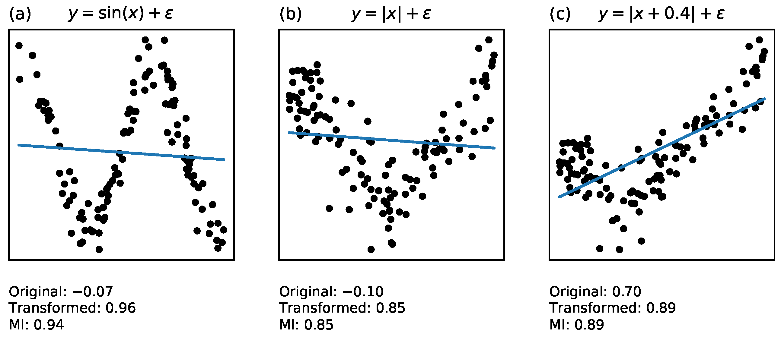
Some examples of non-linear relationships are presented in Figure 1. In all of these cases, Pearson correlation initially fails, but a transformation of the x variable makes the relationship linear. Mutual information predicts the final correlation coefficient.
MI can also be calculated when one or both of the variables is categorical. For example, in [8] the coefficient is calculated between a categorical variable (new particle formation event class) and several continuous variables. In this case, MI is bounded by the finite entropy of the categorical variable, and thus the largest possible correlation in (3) is strictly less than 1. Comparisons between correlations are only valid when the categorical variable is kept fixed, which is the case in the cited article.
2.2. Removing Known Effects
Partial correlation describes the residual dependency between X and Y after removing the effect of some other variable Z. This is done by fitting linear models and and then computing the correlation between model residuals.
A similar procedure can be applied to MI [16], yielding partial or conditional mutual information. Its interpretation is exactly as before: the amount of information shared by X and Y after removing any knowledge gained from Z. It is calculated as in Equation (1), but the probability density is replaced by conditional probability density. After some algebraic manipulation, the conditional MI can be written as
Remarkably, the MI correlation coefficient calculated from conditional MI corresponds exactly to the partial correlation coefficient when the model is linear. The previous transformation invariance property holds as well. The importance of these properties is further illustrated in the case study of Section 4.1.
2.3. Estimation Methods
In order to compute MI, it is necessary to know the probability densities of the variables. There are several numerical methods to estimate densities from observed data points.
The simplest is a binning approach, where variables are approximated by discrete bins [17]. A more advanced method is based on kernel density estimation [18], typically using the normal distribution as the kernel. A downside of these two methods is that they are sensitive to the estimation parameters (bin size or kernel bandwidth, respectively). This is illustrated in [19] (Figure 2).
Instead, Kraskov et al. [20] proposed a k-nearest-neighbor approach. The dependence of results on the number of neighbors k is usually very weak, and as such a fixed default value suffices. This method has also been extended to conditional MI [16] and MI between discrete and continuous variables [19].
We have implemented the nearest-neighbor method and its variants in the open-source Python package ennemi [9]. This package provides several convenient features:
- Ordinary and conditional MI,
- Simple programming interface for common analysis tasks,
- Analysis of time dependency with lags,
- Support for both discrete and continuous variables,
- Optional integration with pandas data frames,
- Efficient, parallel, and tested algorithms.
The package is available on Python Package Index (PyPI). All the analyses in this article were performed with ennemi 1.2.0, SciPy 1.8.0, NumPy 1.22.2, pandas 1.4.1, and Python 3.9.7. The default number of neighbors was used for all analyses.
3. Examples
3.1. Sample Size and Accuracy
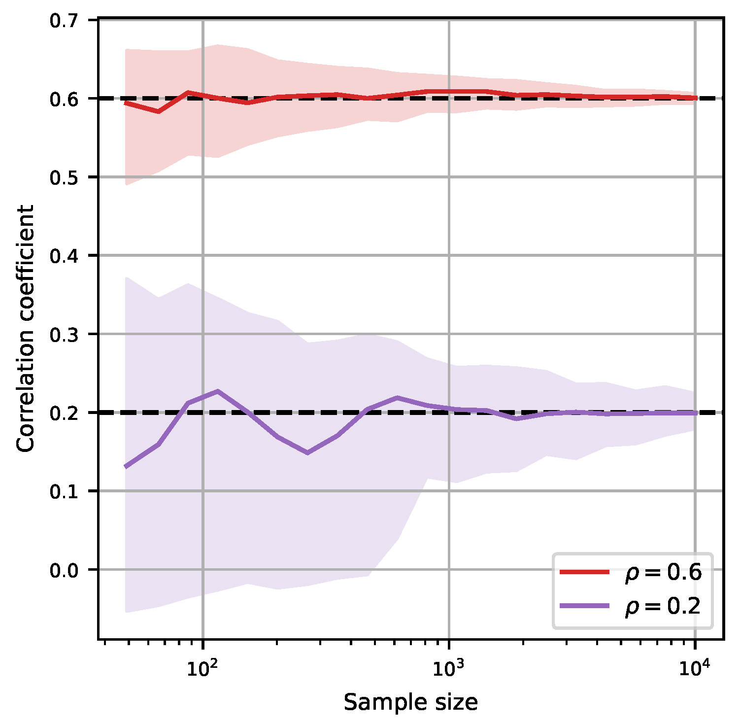
A disadvantage of MI is that it needs more samples than Pearson correlation to produce accurate results. This is because Pearson correlation has implicit knowledge about the model; namely, that it is linear with Gaussian residuals. Figure 2 shows the 50% interval for repeated estimations of two correlated Gaussian variables. It appears that a few hundred data points are necessary to get results correct to one decimal place when the actual correlation is . Due to the nonlinear normalization formula (3), lower correlation values have higher uncertainty. Conditional MI decreases accuracy further.
However, our goal for MI is to screen for most relevant correlations. For this purpose, the achieved precision is good enough. To make the estimate more accurate, methods such as bootstrapping can be used to account for random estimation errors.
On the other hand, very large datasets run into performance issues. A single estimate with 20,000 samples takes approximately 0.2 s on a laptop computer with an Intel i5-1135G7 processor (clock speed 2.40 GHz). Conditioning on one or more variables further increases execution time; see [9] (Figure 1). Again, very large samples are not necessary for initial data exploration; in this article the largest sample contains 10,000 data points.
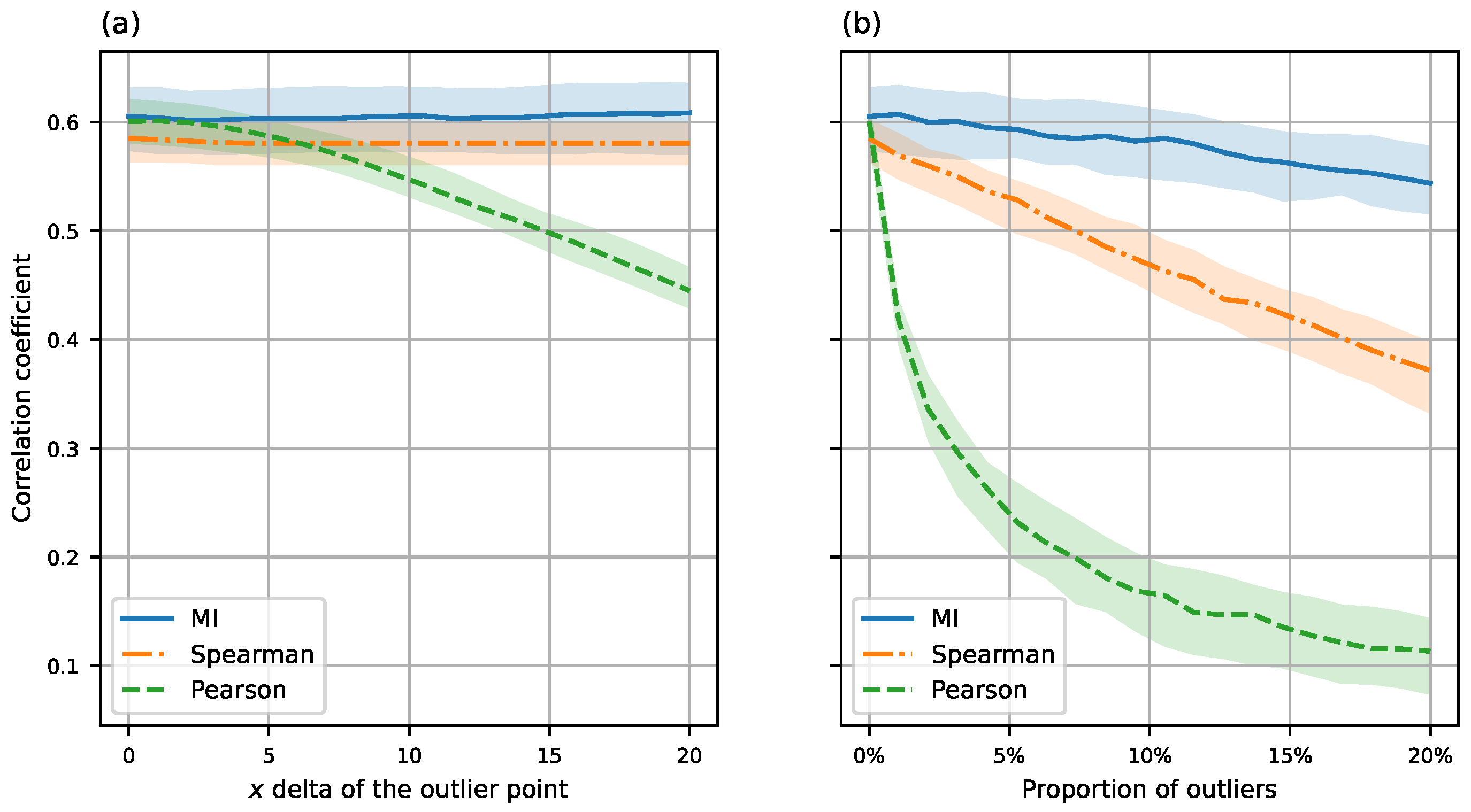
3.2. Robustness
MI correlation appears to be roughly as robust to outliers as Spearman rank correlation. We are not aware of theoretical bounds for, e.g., the breakdown point.
In Figure 3, the effect of both a single outlier and an increasing number of outliers is shown. We simulated data sets of 500 observations from a bivariate normal distribution with marginal variance and correlation . In panel (a), we increased the x coordinate of a single observation to produce an outlier. In panel (b), we moved an increasing proportion of points to .
It is evident that Pearson correlation is not robust in either case, whereas Spearman and MI correlation are not affected by the single diverging point, and MI is the least affected by either scenario.
If the data are recorded at low precision, it might contain identical observations. The nearest-neighbor method may produce incorrect results in this case, because it assumes the probability of two identical observations to be zero. Our package solves this problem by adding low-amplitude noise to the data.
The distribution of a variable may also be censored, for example by the values being close to the measurement threshold. In that case, the same issue occurs. As Figure 3b illustrates, our estimator still produces correct results. Censored measurements are present in the case study of Section 4.2.
3.3. Transformation Invariance
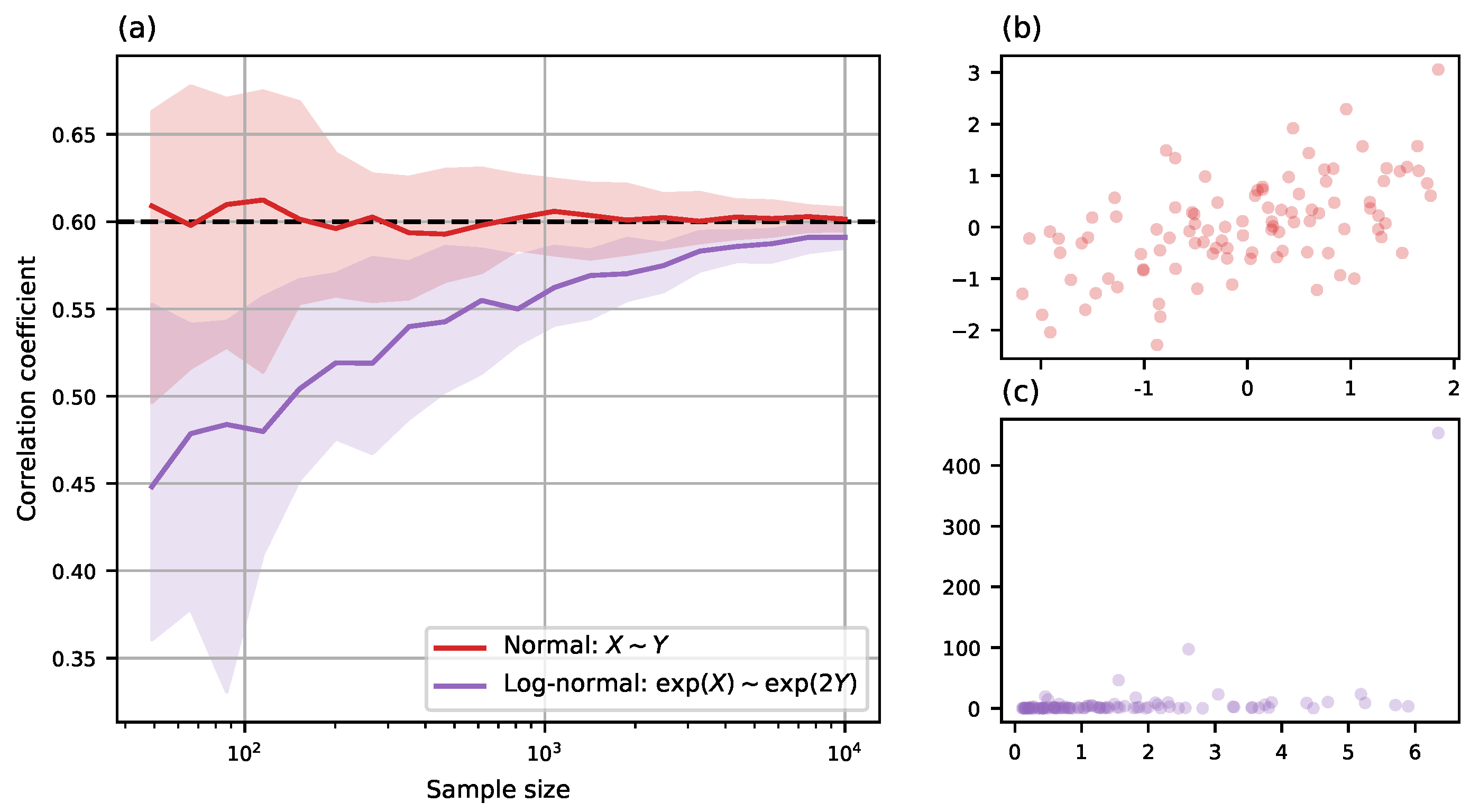
As noted in Section 2.1, the value of MI does not depend on transformations of variables or the shape of their distributions. That is, the MI between and is theoretically the same as between X and Y. This allows us to discover potential correlations without any model specification.
However, the nearest-neighbor estimator does suffer from skewed distributions; effectively, the density estimate becomes too weak at tails. In atmospheric sciences, the most common such distribution is log-normal: if X is normally distributed, then is log-normal. In practice, it is that is observed, and thus it is necessary to take the logarithm to get a less skewed distribution. Figure 4 shows the much faster convergence to correct correlation as a function of sample size when X and Y are normal, as opposed to log-normal and .
While this may appear to counteract the benefit of MI, this transformation only needs to be done once per variable, not once for each variable pair. In practice, this is easy to do as part of data preprocessing. For example, atmospheric trace gas and aerosol concentrations are generally known to follow log-normal distributions and should be log-transformed. We have found other transforms, e.g., square root, much less necessary.
As a rough guideline, each variable should have a somewhat symmetric histogram without heavy tails. Normality is not required. Our software automatically rescales all variables to unit standard deviation, which also improves accuracy slightly.
3.4. Autocorrelated Data
The most severe practical issue is related to autocorrelated data, which of course includes most atmospheric time series. The MI estimation algorithm assumes samples to be independent of each other. The presence of autocorrelation introduces patterns that cause the algorithm to over-estimate the probability density, as illustrated in Figure 5. This leads to a significant positive bias in the MI correlation.
In the case studies below, we apply two methods to remove the autocorrelation bias. In both cases, the solution reduces the sample rate of observations and consequently the sample size. We have used only one data point per day, but 2–3 data points per day is probably still valid for basic meteorological variables. Determination of the safe sample rate should be done on a case-by-case basis.
The first method in used in Section 4.1, where we fix the time of initial observation to 15:00 local time. The mask and lag functions of ennemi compare these observations to the corresponding measurements at h. This procedure immediately reduces the sample rate to one point per day, and gives accurate information on autocorrelations back from the specified time point. Conversely, it gives no information on other times of day.
In Section 4.2, we instead randomly sample a small fraction of data points. Thanks to a large data set, the sample size is still very large. On average, the sample rate is still about one point per day, but all times of day are now represented. This allows us to see the effect of diurnal variation.
The loss in sample size can be compensated by bootstrapping. In the second method, correlation coefficients from several random samples are averaged. In the first method, we can choose for each day a random data point close to the fixed time.
4. Case Studies
Python source code for these case studies, as well as the figures of previous sections, is included in Supplementary Materials. The full data set for Section 4.1 and a reduced data set for Section 4.2 are also included.
4.1. Removing Seasonal Dependency
This example illustrates how a seasonal effect is removed with conditional MI. The results are shown in Figure 6.
We consider a very simplified model for the predictability of weather: given a temperature measurement at 15:00 local time, we estimate its correlation with future temperature measurements. As no other variables are included in the model, the autocorrelation represents the general rate of variability of temperature.
We used hourly temperature observations at Helsinki Kaisaniemi measurement station in Finland from 1 January 2015 to 31 December 2019. In total, the data set contains 1826 days of observations.
We loaded the data into a pandas data frame and linearly interpolated the 15 missing hourly values (only 2 of them were consecutive). As the temperature distribution was fairly symmetric, there was no need to transform the variable.
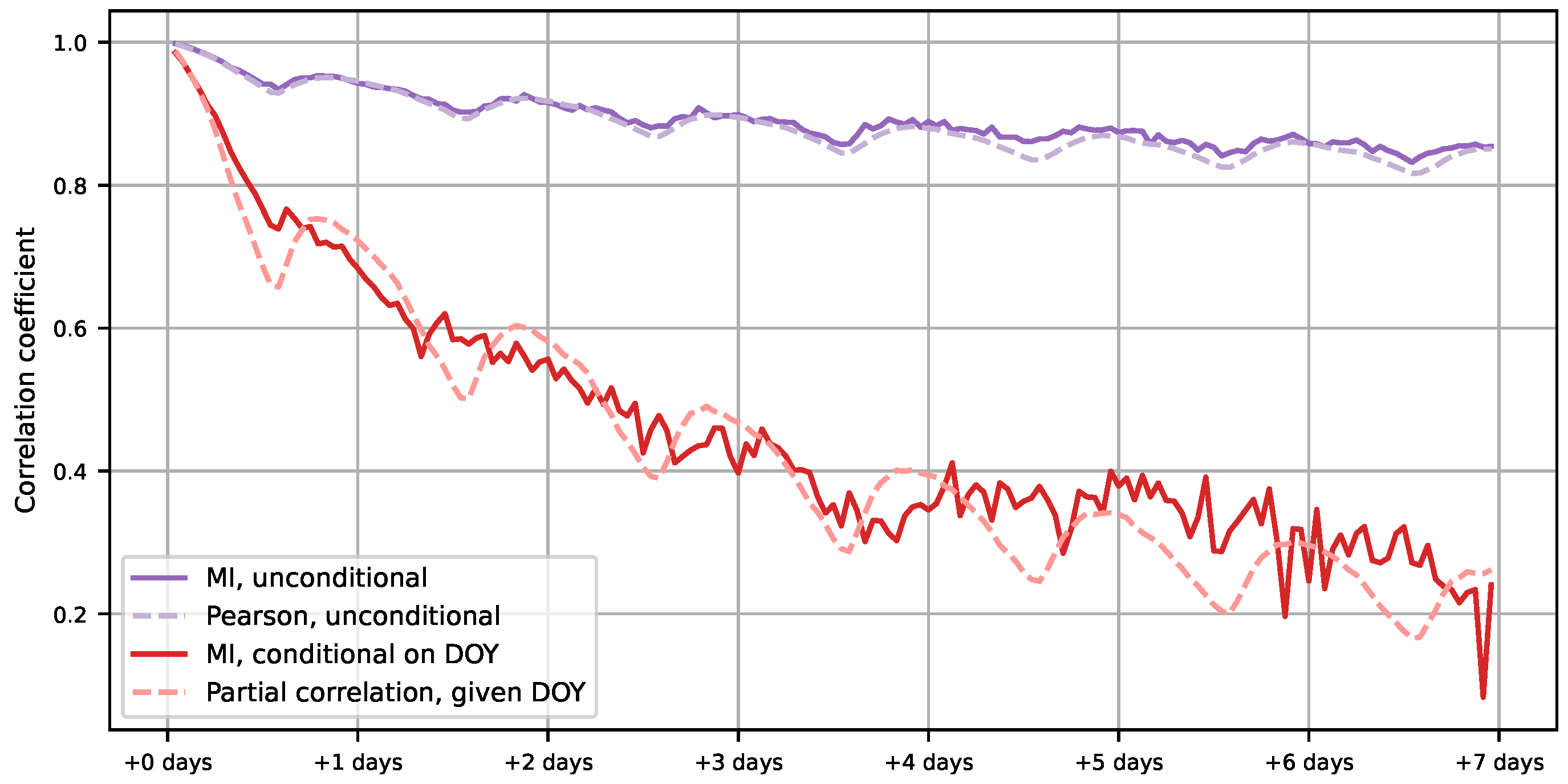
To estimate the MI correlation, we used the estimate_corr method of our ennemi package. We fixed the start time by passing an observation mask that only included the 15:00 (UTC+2) points. We then passed the temperature data as both the x and y parameter, and used the lag parameter to apply a sequence of time differences.
As seen in the top two lines of Figure 6, Pearson and MI correlations are nearly identical. This also illustrates an issue with the straightforward approach: at latitude, the temperature and season are too strongly correlated for day-to-day variation to be visible.
To remove the seasonal effect, we must calculate partial correlation given the day of year. We created a simple seasonal model that incorporates yearly and half-yearly cycles:
Here, t corresponds to the day of year. We fitted the parameters , , , , and c to minimize the sum of squared errors and then repeated the correlation calculation with model residuals instead of observed temperatures. Leap days could be neglected with no loss of accuracy.
For conditional MI, the procedure was rather simpler: we passed an auxiliary “day of year” variable as the cond parameter to the function call. The seasonal effect is then estimated from probability density without an explicit model; in theory, it should yield perfect deseasonalization.
As the bottom two lines in Figure 6 show, the conditional MI correlation coefficient closely matches partial correlation. The deseasonalized correlation decays rapidly, indicating that most temperature patterns only last for a few days. The similarity of the two coefficients suggests that the correlations are close to linear.
The deseasonalization model in Equation (5) is very simple and does not take, e.g., diurnal variation into account at all. At the same time, conditional MI produces equivalent results without any model specification apart from selecting the conditioning variable. Our implementation also supports conditioning simultaneously on multiple variables.
4.2. Discovering Associations across Many Variables
To explore possible dependencies between atmospheric variables, we used measurements from the SMEAR II station located at Hyytiälä Forestry Field Station in Southern Finland, about 50 km northeast from Tampere [1]. Our goal was to benchmark the method with known cross-correlations between variables. Many of these variables are factors related to atmospheric new particle formation (NPF), which is a complex and still not completely understood process [21].
We utilized observations of particle number–size distributions (in the size range 3–1000 nm), several trace gas concentrations (, , , ), and basic meteorology (temperature, wind speed and direction, relative humidity) and global radiation (GlobRad) variables. Measured particle-number size distributions were used to calculate the formation rate of nucleation mode particles (diameter 3–25 nm) and the condensation sink (CS), which describes the loss rate of vapor molecules and small particles due to larger pre-existing particles [22]. Additionally, we used a proxy for the concentration of sulfuric acid, which is known to be connected with atmospheric NPF [23].
The data set ranged from 1 January 1997 to 31 December 2019 with 1 h time resolution. Individual variable availability was 57% to 96% in this interval. By visual inspection of histograms, we chose to take logarithms of the following variables: particle concentration and formation rate, GlobRad, sulfuric acid proxy, , , and CS.
If we were to use the full data set for MI estimation, the autocorrelation issue described in Section 3.4 would lead to extremely biased results. Instead, we randomly sampled 5% (ca. 9800 data points) of the data set, for an average of data points per day. To compensate for loss of precision, we averaged correlation coefficients from three such random samples. The standard deviations of the MI results for most variable pairs match the results shown in Figure 2 for this sample size. More bootstrap iterations could have been used to reduce the uncertainty of the MI estimations, but the present accuracy suffices for data exploration purposes and the computations can be performed within a minute.
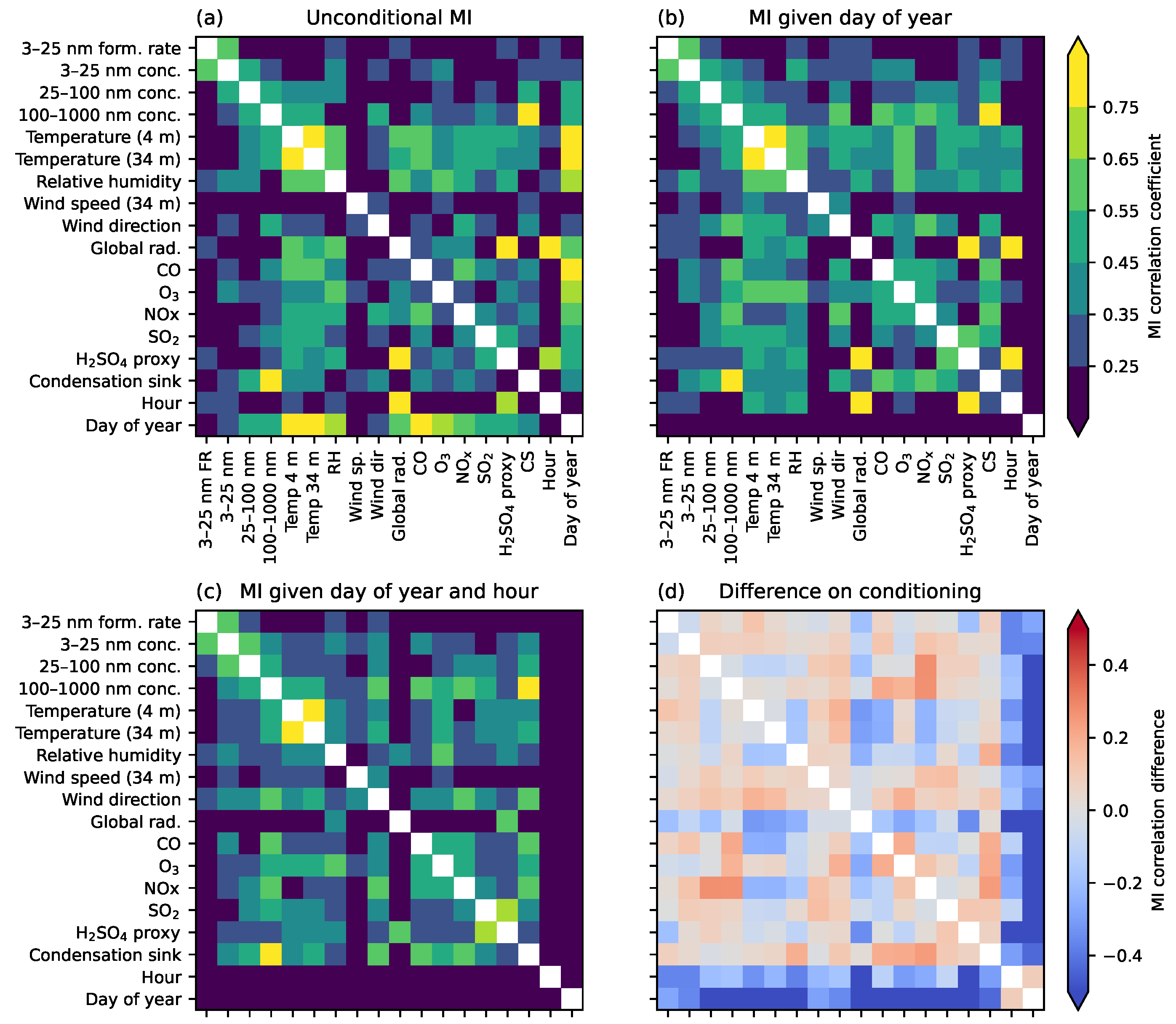
Figure 7 shows the cross-correlation between variables, as given by the pairwise_corr method of ennemi. In the unconditional plot (a), the strong seasonal cycles of several variables are clearly visible by their high MI correlation with the day of year. As expected, the temperature is most correlated with season, followed by trace gases with known seasonal cycles. Only the formation rate of 3–25 nm particles and wind speed/direction are only weakly correlated with day of year.
Conditioning on day of year removes the seasonal cycle of each variable. We can see from Figure 7b that another natural cycle still remains: the time of day is strongly correlated with temperature, radiation, and some other variables. This obvious correlation can be removed by conditioning simultaneously on both the date and time. In Figure 7c, only the variations unexplained by yearly and daily cycles remain.
Comparison of the matrices reveals that most of the correlations with global radiation are actually explained by date and time, and that only relative humidity and the sulfuric acid proxy correlate with deseasonalized GlobRad. The sulfuric acid proxy is a function of GlobRad, , , and condensation sink. All of these are identified in Figure 7b–c. The other correlations with sulfuric acid are partly explained by common factors, such as the cross-correlation of with , or GlobRad/CS with time. As sulfuric acid is a precursor to nucleation-mode particles, its correlation with particle number also matches our expectations.
The interpretation of conditional MI results requires some care. For instance, we see a correlation between the sulfuric acid proxy concentration and particle formation rate in Figure 7a,b, but not in Figure 7c. This does not indicate that sulfuric acid and particle formation rate are unrelated; rather, both of them have similar diurnal cycles with maximum in the daytime and minimum in the nighttime. The figures suggest that (a) there is a relationship between the two variables; (b) the relationship remains strong within each season; (c) but day-to-day variation in sulfuric acid is less significant in explaining the particle formation rate. MI cannot distinguish whether the two variables are causally related, or both explained by a common factor (date and time, similar long-term trend, third variable, etc.). Some of the correlations shown in Figure 7 are weaker than previously reported in SMEAR II station [21], but the difference is explained by the unconstrained data set analyzed here.
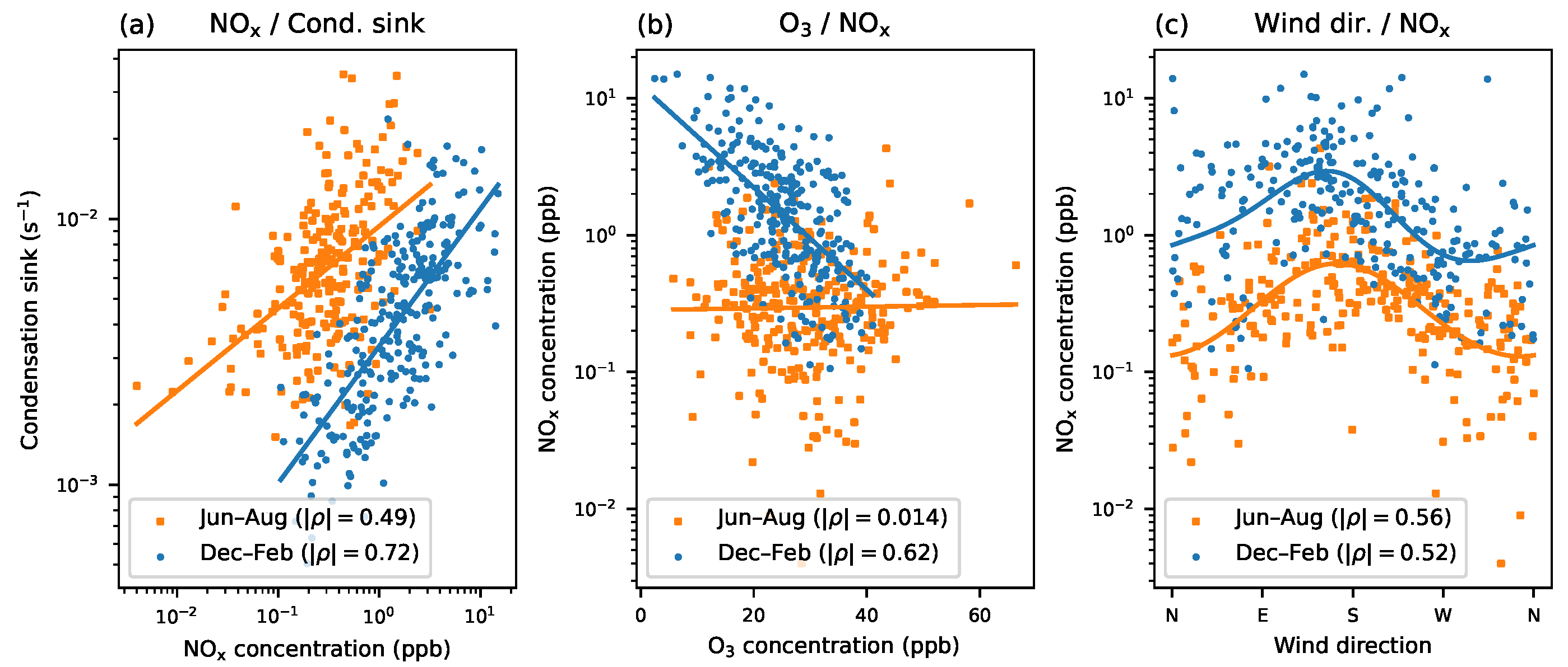
Most importantly, the functional relationships between the studied variables can be arbitrary. Some examples are shown in Figure 8. In panels (a) and (b), one or both of the variables are on a logarithmic axis, which must be taken into account when fitting a line. In panel (c) one of the variables is wind direction, which is a circular variable. A more specialized model is needed here; we opted for an analogue of Equation (5) to produce the fit line in the figure. This illustrates the main benefit of MI: sensible correlation values are given without the need to choose and justify a model.
We were also interested in possible time dependencies between the variables. For example, it takes some time for a newly formed particle to grow large enough for detection. It would hence make sense to apply a lag to the covariate measurements. As in Section 4.1, we used the estimate_corr method to produce figures of correlations at different lag values. The method accepts a mask parameter that selects a subset of data without destroying the time series structure.
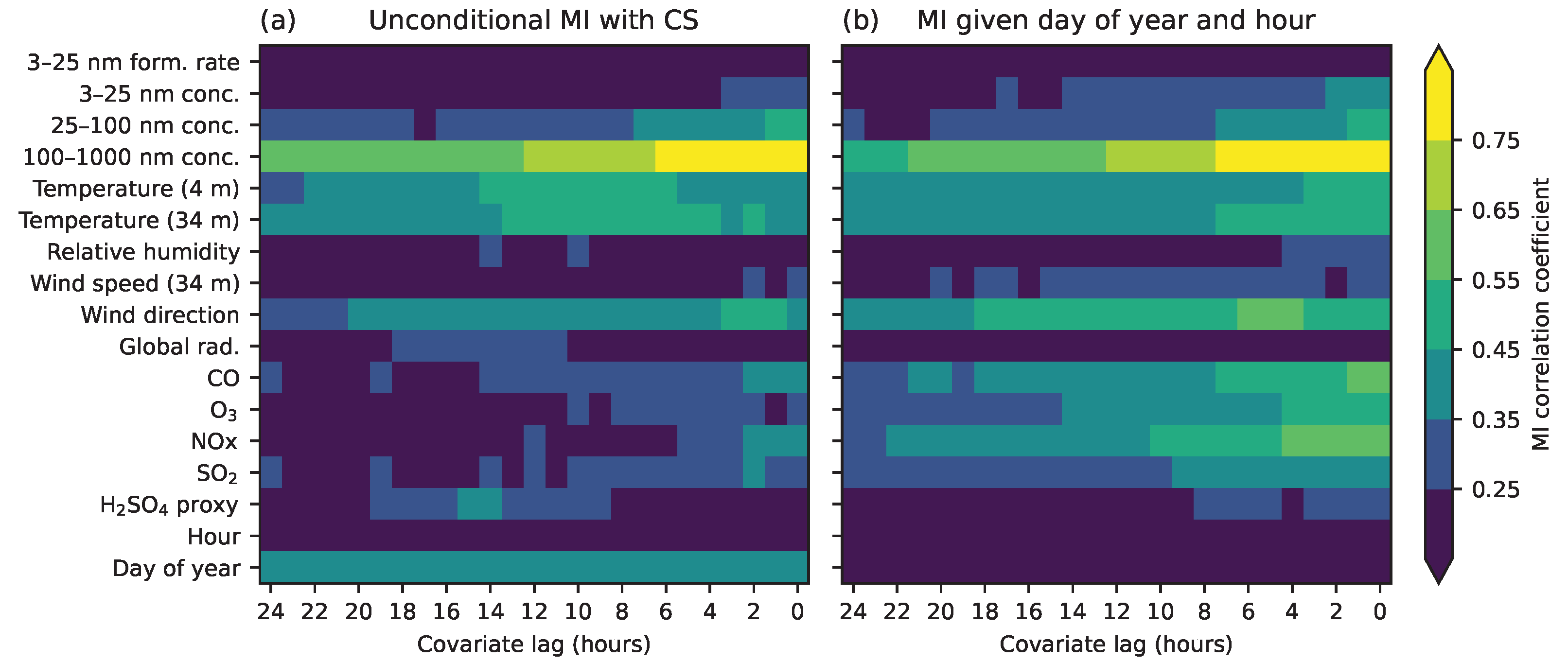
Figure 9 presents the time-dependent correlations of condensation sink and the other variables. We see that correlations are generally strongest when there is no time difference between the variables. The rate of decay corresponds to the rate of change (autocorrelation) of each variable. The highest MI values are observed between CS and the concentration of 100–1000 nm accumulation mode particles, which is an expected result given the typical particle size-distributions observed at the Hyytiälä SMEAR station [25]. The correlation of CS with wind direction seems to be strongest some 4–6 h before the CS measurement, however visual inspection of scatter plots between these variables suggests that the differences in the correlations at different lag times are not very large.
5. Conclusions
Several features make mutual information an attractive method for exploratory data analysis of atmospheric variables. In particular, the measure is robust to outliers and unprecise or censored data. The MI correlation coefficient matches Pearson correlation exactly in many cases that traditionally require transformations of variables.
We also discussed some practical issues and limitations with MI. Autocorrelated data, as is common in atmospheric sciences, pose problems that must be addressed in the analysis workflow, e.g., by suitably sampling from the original dataset. Some care is thus necessary when using the method with time series data. Low MI correlation values are accurate only when the sample sizes are large. While the MI algorithm is more computationally intensive than the classical methods, execution time is not an issue in practice even with large datasets.
We performed several case studies to evaluate the method. We found that the method makes it easy to detect non-linear relationships that would otherwise require model specification or visualization: instead of modeling variable pairs, possibly conditional on other variables, it suffices to quality-check the N variables. With the ever-increasing number of datasets of environmental variables available, pairwise MI plots help focus on exploring the most relevant connections. Time-lag plots and conditioning can be used to suggest causal relationships.
Let us still summarize the analysis workflow we used in our case studies:
- 1.
- After the usual data quality checking, preprocess variables to have roughly symmetric histograms. Select a suitable subset of autocorrelated data.
- 2.
- Estimate pairwise MI between all variables, as in Figure 7.
- 3.
- Use conditional MI to investigate common factors such as seasonal cycles.
- 4.
- Estimate time dependencies with the variables of interest, as in Figure 9.
- 5.
- Draw scatter plots and manually explore the reduced set of the most interesting variables.
Our Python package is designed to support this workflow. As the method requires little data preparation or technical tweaking, it should be easy to try out on various data sets. While the case studies presented in our work are within atmospheric sciences, the methods are applicable to other fields of natural science as well. Some additional features of the package are described in its online documentation (https://polsys.github.io/ennemi/, accessed on 21 June 2022). In particular, the package also supports categorical variables.
With the large datasets now available, it is possible to “mine” for new hypotheses and associations between variables. Our workflow makes the process easier and helps guide modeling efforts.
Supplementary Materials
The following supporting information can be downloaded at: https://www.mdpi.com/article/10.3390/atmos13071046/s1. Derivations of theoretical results. Source code and partial data for all the figures.
Author Contributions
P.L. wrote the software, analyzed and visualized the data, and wrote the article. E.A. analyzed the data and contributed to the writing. M.A.Z. conceptualized the study and contributed to the writing. S.M. contributed to the writing. T.N. interpreted the data, led the project, and contributed to the writing. All authors have read and agreed to the published version of the manuscript.
Funding
This work was supported by Academy of Finland PROFI3 funding (decision number 311932). SM was supported by Academy of Finland Flagship funding (337550). Open access funding was provided by University of Helsinki Library.
Institutional Review Board Statement
Not applicable.
Informed Consent Statement
Not applicable.
Data Availability Statement
The data for Section 4.1 is available from Finnish Meteorological Institute under CC-BY 4.0 license (https://en.ilmatieteenlaitos.fi/download-observations, accessed on 21 June 2022) and included in Supplementary Materials. The data for Section 4.2 is available on SmartSMEAR under CC-BY 4.0 licence (https://smear.avaa.csc.fi/, accessed on 21 June 2022). Formation rates, condensation sink, and sulfuric acid proxy are computed from the data and not available on SmartSMEAR. A subset of the data is included in Supplementary Materials.
Conflicts of Interest
The authors declare no conflict of interest.
References
- Hari, P.; Kulmala, M. Station for Measuring Ecosystem–Atmosphere Relations (SMEAR II). Boreal Environ. Res. 2005, 10, 315–322. [Google Scholar]
- Kulmala, M.; Nieminen, T.; Nikandrova, A.; Lehtipalo, K.; Manninen, H.E.; Kajos, M.K.; Kolari, P.; Lauri, A.; Petäjä, T.; Krejci, R.; et al. CO2-induced terrestrial climate feedback mechanism: From carbon sink to aerosol source and back. Boreal Environ. Res. 2014, 19, 122–131. [Google Scholar]
- Battiti, R. Using mutual information for selecting features in supervised neural net learning. IEEE Trans. Neural Netw. 1994, 5, 537–550. [Google Scholar] [CrossRef] [PubMed] [Green Version]
- Pluim, J.; Maintz, J.; Viergever, M. Mutual-information-based registration of medical images: A survey. IEEE Trans. Med. Imaging 2003, 22, 986–1004. [Google Scholar] [CrossRef]
- Zaidan, M.A.; Dada, L.; Alghamdi, M.A.; Al-Jeelani, H.; Lihavainen, H.; Hyvärinen, A.; Hussein, T. Mutual information input selector and probabilistic machine learning utilisation for air pollution proxies. Appl. Sci. 2019, 9, 4475. [Google Scholar] [CrossRef] [Green Version]
- Guo, X.; Zhang, H.; Tian, T. Development of stock correlation networks using mutual information and financial big data. PLoS ONE 2018, 13, e0195941. [Google Scholar] [CrossRef]
- Basso, K.; Margolin, A.A.; Stolovitzky, G.; Klein, U.; Dalla-Favera, R.; Califano, A. Reverse engineering of regulatory networks in human B cells. Nat. Genet. 2005, 37, 382–390. [Google Scholar] [CrossRef]
- Zaidan, M.A.; Haapasilta, V.; Relan, R.; Paasonen, P.; Kerminen, V.M.; Junninen, H.; Kulmala, M.; Foster, A.S. Exploring non-linear associations between atmospheric new-particle formation and ambient variables: A mutual information approach. Atmos. Chem. Phys. 2018, 18, 12699–12714. [Google Scholar] [CrossRef] [Green Version]
- Laarne, P.; Zaidan, M.A.; Nieminen, T. ennemi: Non-linear correlation detection with mutual information. SoftwareX 2021, 14, 100686. [Google Scholar] [CrossRef]
- Ulpiani, G.; Ranzi, G.; Santamouris, M. Local synergies and antagonisms between meteorological factors and air pollution: A 15-year comprehensive study in the Sydney region. Sci. Total Environ. 2021, 788, 147783. [Google Scholar] [CrossRef]
- Ulpiani, G.; Nazarian, N.; Zhang, F.; Pettit, C.J. Towards a living lab for enhanced thermal comfort and air quality: Analyses of standard occupancy, weather extremes, and COVID-19 pandemic. Front. Environ. Sci. 2021, 9, 556. [Google Scholar] [CrossRef]
- Cover, T.M.; Thomas, J.A. Elements of Information Theory; Wiley-Interscience: Hoboken, NJ, USA, 2006. [Google Scholar]
- Ihara, S. Information Theory for Continuous Systems; World Scientific: Singapore, 1993. [Google Scholar]
- Linfoot, E.H. An informational measure of correlation. Inf. Control 1957, 1, 85–89. [Google Scholar] [CrossRef] [Green Version]
- Granger, C.; Lin, J.L. Using the mutual information coefficient to identify lags in nonlinear models. J. Time Ser. Anal. 1994, 15, 371–384. [Google Scholar] [CrossRef]
- Frenzel, S.; Pompe, B. Partial mutual information for coupling analysis of multivariate time series. Phys. Rev. Lett. 2007, 99, 204101. [Google Scholar] [CrossRef] [PubMed]
- Fraser, A.M.; Swinney, H.L. Independent coordinates for strange attractors from mutual information. Phys. Rev. A 1986, 33, 1134–1140. [Google Scholar] [CrossRef]
- Moon, Y.I.; Rajagopalan, B.; Lall, U. Estimation of mutual information using kernel density estimators. Phys. Rev. E 1995, 52, 2318–2321. [Google Scholar] [CrossRef]
- Ross, B.C. Mutual information between discrete and continuous data sets. PLoS ONE 2014, 9, e87357. [Google Scholar] [CrossRef]
- Kraskov, A.; Stögbauer, H.; Grassberger, P. Estimating mutual information. Phys. Rev. E 2004, 69, 066138. [Google Scholar] [CrossRef] [Green Version]
- Dada, L.; Paasonen, P.; Nieminen, T.; Buenrostro Mazon, S.; Kontkanen, J.; Peräkylä, O.; Lehtipalo, K.; Hussein, T.; Petäjä, T.; Kerminen, V.M.; et al. Long-term analysis of clear-sky new particle formation events and nonevents in Hyytiälä. Atmos. Chem. Phys. 2017, 17, 6227–6241. [Google Scholar] [CrossRef] [Green Version]
- Kulmala, M.; Petäjä, T.; Nieminen, T.; Sipilä, M.; Manninen, H.E.; Lehtipalo, K.; Dal Maso, M.; Aalto, P.P.; Junninen, H.; Paasonen, P.; et al. Measurement of the nucleation of atmospheric aerosol particles. Nat. Protoc. 2012, 7, 1651–1667. [Google Scholar] [CrossRef]
- Dada, L.; Ylivinkka, I.; Baalbaki, R.; Li, C.; Guo, Y.; Yan, C.; Yao, L.; Sarnela, N.; Jokinen, T.; Daellenbach, K.R.; et al. Sources and sinks driving sulfuric acid concentrations in contrasting environments: Implications on proxy calculations. Atmos. Chem. Phys. 2020, 20, 11747–11766. [Google Scholar] [CrossRef]
- Riuttanen, L.; Hulkkonen, M.; Dal Maso, M.; Junninen, H.; Kulmala, M. Trajectory analysis of atmospheric transport of fine particles, SO2, NOx and O3 to the SMEAR II station in Finland in 1996–2008. Atmos. Chem. Phys. 2013, 13, 2153–2164. [Google Scholar] [CrossRef] [Green Version]
- Lehtinen, K.E.J.; Korhonen, H.; Dal Maso, M.; Kulmala, M. On the concept of condensation sink diameter. Boreal Environ. Res. 2003, 8, 405–411. [Google Scholar]
Figure 1.
Examples of best linear fit lines (blue solid lines) to three different types of non-linear relationships, the Pearson correlation coefficient before and after transforming the x variable, and the MI correlation. Each sample has 120 points (a–c).
Figure 1.
Examples of best linear fit lines (blue solid lines) to three different types of non-linear relationships, the Pearson correlation coefficient before and after transforming the x variable, and the MI correlation. Each sample has 120 points (a–c).

Figure 2.
Median and interquartile range of MI correlation coefficient as the sample size increases, for actual correlations and . The low correlation case has more noise from the estimator.
Figure 2.
Median and interquartile range of MI correlation coefficient as the sample size increases, for actual correlations and . The low correlation case has more noise from the estimator.

Figure 3.
Medians and interquartile ranges of various sample () correlation coefficients (a) as the x coordinate of a single point is increased, (b) as the proportion of points with is increased.
Figure 3.
Medians and interquartile ranges of various sample () correlation coefficients (a) as the x coordinate of a single point is increased, (b) as the proportion of points with is increased.

Figure 4.
(a) Median and interquartile range of MI correlation coefficient as the sample size increases. The bottom line is of two log-normal variables; the top line of the same variables after a log transform is much closer to the real . (b) A sample from the correlated normal distributions of X and Y values is quite symmetric. (c) The corresponding log-normal distribution of the values and is concentrated near the origin but has many far-away points, as illustrated by the larger axis range (maximal ).

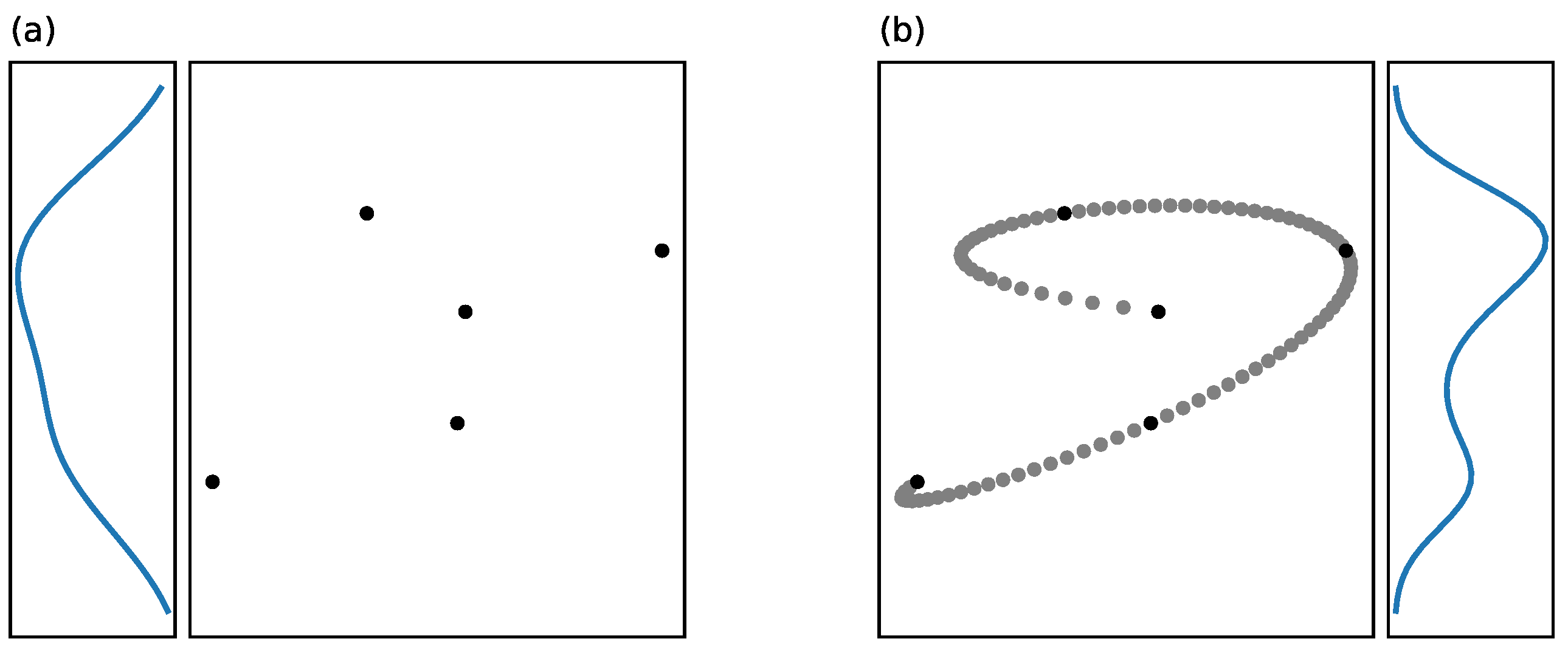
Figure 5.
(a) Five observations of independent variables. The outer panel shows the probability density of the y variable given by Gaussian kernel density estimation, with zero along the inner edge. The estimated density is smooth. (b) Polynomial interpolation through the points creates a pattern. Marginal density has peaks as the estimator bandwidth is smaller. Default bandwidth selection of SciPy was used.

Figure 6.
MI (solid lines) and Pearson correlation (dashed lines) between temperature measured at 15:00 and hourly temperature measurements up to 7 days after this. The top two lines are results without deseasonalization and the bottom two take seasonality into account.
Figure 6.
MI (solid lines) and Pearson correlation (dashed lines) between temperature measured at 15:00 and hourly temperature measurements up to 7 days after this. The top two lines are results without deseasonalization and the bottom two take seasonality into account.

Figure 7.
Pairwise MI correlation between a selection of SMEAR II variables. Correlation values below are not shown. (a) The bottom two rows of unconditional MI indicate that many variables have strong seasonal and diurnal cycles. (b) Conditioning on the day of year removes the seasonal cycles. The explanative strength of diurnal cycles is increased. (c) Additionally conditioning on the hour removes diurnal cycles as well. The correlations are related to any remaining variation in the variables. Other common factors may still exist, however. (d) By comparing subfigures (a,c), we see that especially the effect of global radiation is actually explained by date and time. After conditioning, a strong correlation only remains with the sulfuric acid proxy, of which global radiation is an input, and with relative humidity. Conversely, the wind direction (air mass source) gains explanative power when usual yearly variations are removed.

Figure 8.
Examples of non-linear correlations related to trace gases and condensation sink. Observations are separated by season, but a random sample from all times of day is used. The correlation coefficient refers to each fitted non-linear model. (a) Condensation sink and concentration of nitrous oxides are both logarithmic variables. A log-log-linear model explains their correlation. Conditional MI from Figure 7b is . (b) Ozone follows a linear scale. The log-linear correlation between and depends heavily on the season. Conditional MI is . (c) Wind direction versus logarithmic concentration. A two-level trigonometric model analogous to Equation (5) is fitted. Conditional MI is . Existing literature suggests that wind direction explains all three other variables [24].

Figure 9.
Correlation coefficients between studied variables and the condensation sink (CS) as function of the lag time for (a) unconditional MI and (b) conditioning on season and time of day. Covariates are measured at times up to 24 h before the CS observation. The correlation with sulfuric acid proxy is most likely explained by similar diurnal variation, as it is reduced by conditioning on the time of day.

Publisher’s Note: MDPI stays neutral with regard to jurisdictional claims in published maps and institutional affiliations. |
© 2022 by the authors. Licensee MDPI, Basel, Switzerland. This article is an open access article distributed under the terms and conditions of the Creative Commons Attribution (CC BY) license (https://creativecommons.org/licenses/by/4.0/).
Share and Cite
MDPI and ACS Style
Laarne, P.; Amnell, E.; Zaidan, M.A.; Mikkonen, S.; Nieminen, T. Exploring Non-Linear Dependencies in Atmospheric Data with Mutual Information. Atmosphere 2022, 13, 1046. https://doi.org/10.3390/atmos13071046
AMA Style
Laarne P, Amnell E, Zaidan MA, Mikkonen S, Nieminen T. Exploring Non-Linear Dependencies in Atmospheric Data with Mutual Information. Atmosphere. 2022; 13(7):1046. https://doi.org/10.3390/atmos13071046
Chicago/Turabian StyleLaarne, Petri, Emil Amnell, Martha Arbayani Zaidan, Santtu Mikkonen, and Tuomo Nieminen. 2022. "Exploring Non-Linear Dependencies in Atmospheric Data with Mutual Information" Atmosphere 13, no. 7: 1046. https://doi.org/10.3390/atmos13071046
Note that from the first issue of 2016, this journal uses article numbers instead of page numbers. See further details here.