
Nitrous Oxide Profile Retrievals from Atmospheric Infrared Sounder and Validation
by
Cuihong Chen
1, 
Pengfei Ma
1,*,
Liangfu Chen
2,3,
Yuhuan Zhang
1,
Chunyan Zhou
1,
Shaohua Zhao
1,
Lianhua Zhang
1 and
Zhongting Wang
1,* 1
Satellite Application Center for Ecology and Environment, Ministry of Ecology and Environment of the People’s Republic of China, Beijing 100094, China
2
State Key Laboratory of Remote Sensing Science, Jointly Sponsored by Aerospace Information Research Institute of Chinese Academy of Sciences and Beijing Normal University, Beijing 100101, China
3
University of Chinese Academy of Sciences, Beijing 100049, China
*
Authors to whom correspondence should be addressed.
Atmosphere 2022, 13(4), 619; https://doi.org/10.3390/atmos13040619
Submission received: 29 January 2022
/
Revised: 26 March 2022
/
Accepted: 4 April 2022
/
Published: 12 April 2022
(This article belongs to the Special Issue Recent Advances in Optical Remote Sensing of Atmosphere)
Abstract
:This paper presents an algorithm for the retrieval of nitrous oxide profiles from the Atmospheric InfraRed Sounder (AIRS) on the Earth Observing System (EOS)/Aqua using a nonlinear optimal estimation method. First, an improved Optimal Sensitivity Profile (OSP) algorithm for channel selection is proposed based on the weighting functions and the transmissions of the target gas and interfering gases, with 13 channels selected for inversion in this algorithm. Next, the data of the High-Performance Instrumented Airborne Platform for Environmental Research (HIAPER) Pole-to-Pole Observations (HIPPO) aircraft and the Earth System Research Laboratory (ESRL) are used to verify the retrieval results, including the atmospheric nitrous oxide profile and the column concentration. The results show that using AIRS satellite data, the atmospheric nitrous oxide profile between 300–900 hPa can be well retrieved with an accuracy of ~0.1%, which agrees with the corresponding Jacobian peak interval of selected channels. Analysis of the AIRS retrievals demonstrates that the AIRS measurements provide useful information to capture the spatial and temporal variations in nitrous oxide between 300–900 hPa.
1. Introduction
In the past 40 years, there have been more and more discussions regarding the role of human activities in affecting atmospheric composition and the subsequent consequences. The major concerns of scientists and policy makers are global warming and stratospheric ozone depletion [1]. N2O plays a very important role in these two aspects. On the one hand, it is a very important greenhouse gas. Its 20-year and 100-year global warming potentials (GWPs) and 20-, 50-, and 100-year global temperature change potentials (GTPs) are nearly 300 times that of CO2, although its radiative forcing is far less than CO2 and CH4 [2]. In addition to its radiative forcing on the climate system, since the beginning of the 21st century, N2O has also been viewed as the most important ozone-depleting substance [3].
Traditional ground-based observations cannot provide a global picture of N2O distribution (or geographic variability) because their coverage is sparse. In the past decades, space-borne remote sensing has been employed for the measurement of global nitrous oxide. There are mainly three spectral ranges used to measure N2O: the mid infrared (2265–2280 nm), thermal infrared (4.5–8 μm), and microwave (652.83–502.296 GHz), with three viewing geometries (limb, occultation, and nadir). The limb instruments include the Stratospheric and Mesospheric Sounder (SAMS, on board Nimbus-7) by means of limb measurement [4], the Sub-Millimeter Radiometer (SMR, on board Odin) [5], the Microwave Limb Sounder (MLS, on board Aura) [6], and the Michelson Interferometer for Passive Atmospheric Sounding (MIPAS, on board Envisat) [7], as well as the Atmospheric Chemistry Experiment-Fourier Transform Spectrometer (ACE-FTS, on board SCISAT-1) [8]. The occultation measurements include the Atmospheric Trace Molecule Spectroscopy (ATMOS) on board Atlas-I, -II, and -III [9,10], which is the first measurement of N2O using infrared occultation, and the Improved Limb Atmospheric Spectrometer (ILAS and ILAS-II) on board the Advanced Earth Observing Satellite (ADEOS)-I and ADEOS-II [11].
The limb and occultation observations are mainly focused on the middle and upper atmospheres, while the nadir observation can provide effective information on the troposphere, with a better horizontal resolution and the capability to derive the surface temperature and emissivity via inverse retrieval. The nadir measurements include the Atmospheric Infrared Sounder (AIRS, on board Aqua) [12], the Tropospheric Emission Spectrometer (TES, on board EOS-Aura) [13], the Infrared Atmospheric Sounding Interferometer (IASI, on board MetOp-A) [14], and the Cross-track Infrared Sounder (CrIS, on board Suomi-NPP) [15].
The AIRS, an infrared spectrometer, is designed to produce high-resolution, three-dimensional water vapor and temperature profiles on a global scale. The AIRS on NASA’s Aqua satellite was launched on May 4, 2002. It provides soundings of the atmosphere with 2378 spectral channels over three wavelength ranges, i.e., long-wavelength infrared (LWIR, 8.80–15.4 μm [1136–649 cm−1]), medium-wavelength infrared (MWIR, 6.24–8.22 μm [1613–1216 cm−1]), and short-wavelength infrared (SWIR, 3.74–4.61 μm [2665–2181 cm−1]) at a high spectral resolution (λ/∆λ = 1200) [16]. The large swath on the polar orbiting and the observation at the infrared band makes it possible to provide global observation twice a day, both day and night. Xiong et al. (2014) [12] showed the capability to undertake the retrieval of N2O using the AIRS algorithm. Ma et al. (2021) [17] analyzed the annual and monthly mean changes of nitrous oxide and its spatial distribution characteristics in China for the first time from AIRS data by using the OEM method. Xiong et al. (2014) [12] derived the concentration and change of N2O by using a singular value decomposition (SVD) of the weighted covariance of the sensitivity matrix and damping the least significant eigenfunctions of the SVD to constrain the solution. A different retrieval method, especially the channel selection method, is developed and presented in this paper. In our study, an optimal estimation method [18] is used. Section 2 describes this method, the a priori profile used, the method of channel selection based on the channel sensitivities, and the weighting functions. Validation of the results through comparisons with different data are shown and discussed in Section 3. The summary and conclusions are provided in Section 4. The developed channel selection method in this study can obtain the absorption information of N2O to the greatest extent and improve the inversion accuracy. In addition, AIRS has not released N2O products at present.
2. Materials and Methods
Because the retrieval problem is ill-conditioned and has no unique and stable solution, regularization techniques must be utilized to find the best representation of the true state. The optimal estimation method [18] is one of the most widely used methods for retrieval. This method is adopted to derive nitrous oxide profiles in this paper.
Since the forward model is usually a nonlinear function of the atmospheric state vector, an iterative method is needed to find the minimum of the cost function (J):
The difference between the measured () and the simulated () radiances and the difference between the retrieved () and a priori () state vectors are constrained by the measurement error covariance matrix () and the a priori covariance matrix (), respectively. The solution in each iteration is:
where and are the current and previous state vectors, respectively. In our retrieval scheme, the first guess () is chosen to be equal to the a priori profile (). is the weighting function, or Jacobian matrix. The a priori covariance matrix is used as follows [18,19]:
where i and j are the index of , respectively, H is a scalar (the value here is 1000), and is the standard deviation of the a priori as detailed in Section 2.1. The measurement error covariance matrix () is a diagonal matrix from the AIRS noise [20] and the non-diagonal elements are set to zero.
In our retrieval, the atmospheric temperature, humidity, O3, surface temperature, and surface emissivity data from the AIRS L2 products are used as inputs in the forward model. AIRS L1 cloud-cleared AIRS data are used for retrieval. The N2O profile parameter is the state vector.
2.1. A Priori Profile
For the ill-conditioned problems, other information, in addition to the measurements, is needed to constrain the solution and to choose a reasonable profile from the infinite number of mathematically possible profiles [21]. In the optimal estimation retrieval technique, this information generally takes the form of the a priori profile and Sa matrix, which is regarded as a very important prior restriction to obtain a stabilized and regularized solution [22].
Eigenvector regression method profiles are often used to construct the a priori state. This study investigates an algorithm for rapidly retrieving initial atmospheric N2O profiles from AIRS hyperspectral data based on eigenvector statistics. It mainly includes the following steps: (1) using the community radiative transfer model (CRTM) [23] for rapid brightness temperatures (BTs) simulations and BTs derivative calculations under various sky and surface conditions; (2) performing an empirical orthogonal expansion on the covariance matrix of the simulated BTs using principal components analysis; (3) finding the best fits to the matrix of the profile samples and to the empirically orthogonally expanded matrix of the simulated BTs using the method of least squares and calculating the regression coefficients; and, finally, (4) using the AIRS data to rapidly derive atmospheric N2O profiles based on the regression coefficients, and using it as the initial profile for the optimal estimation algorithm. This method to derive the first guess is similar to the AIRS algorithm in the derivation of temperature and water vapor first guess profile and later use of this profile and AIRS data in a set of channels for the final retrievals [24,25]. So, the difference of this algorithm from the AIRS algorithm is the use of the optimal estimation method for retrieval, and the algorithm in this study obtains a non-fixed first guess through statistical regression, while the first guess of N2O in the AIRS algorithm is a fixed value [12].
The training samples consist of two parts, namely the atmospheric profile samples and BTs, as simulated based on the profile samples. The atmospheric profile samples are composed of 83 global temperature, humidity, CO2, O3, N2O, CO, and CH4 profiles in 101 atmospheric pressure layers under clear-sky conditions [26]. These profiles are sampled from 121,462,560 profiles using the cycle 30R2 model of the European Centre for Medium-Range Weather Forecasts system and the sampling strategy proposed by Chevallier et al. (2006) [27].
Using the simulated BTs () (we select the first 1245 channels (649.50 cm−1 to 1273 cm−1)), the inverse solution can be written [28,29] as:
where the vector contains the atmospheric profiles of the nitrous oxide. is the best fit operator matrix obtained using a linear least-squares method:
where () is the covariance of the simulated BTs, () is the covariance of the training profile with the simulated BTs, and () is the statistical covariance of the spectral radiance noise which is adopted from AIRS with a fixed value for each channel. This method decomposes the sample profile and simulated radiation value at the same time, and couples the principal component coefficient to the regression coefficient, which will reduce the calculation time and the error in the calculation process. The detailed eigenvector regression algorithm was presented in our previous published article [30].
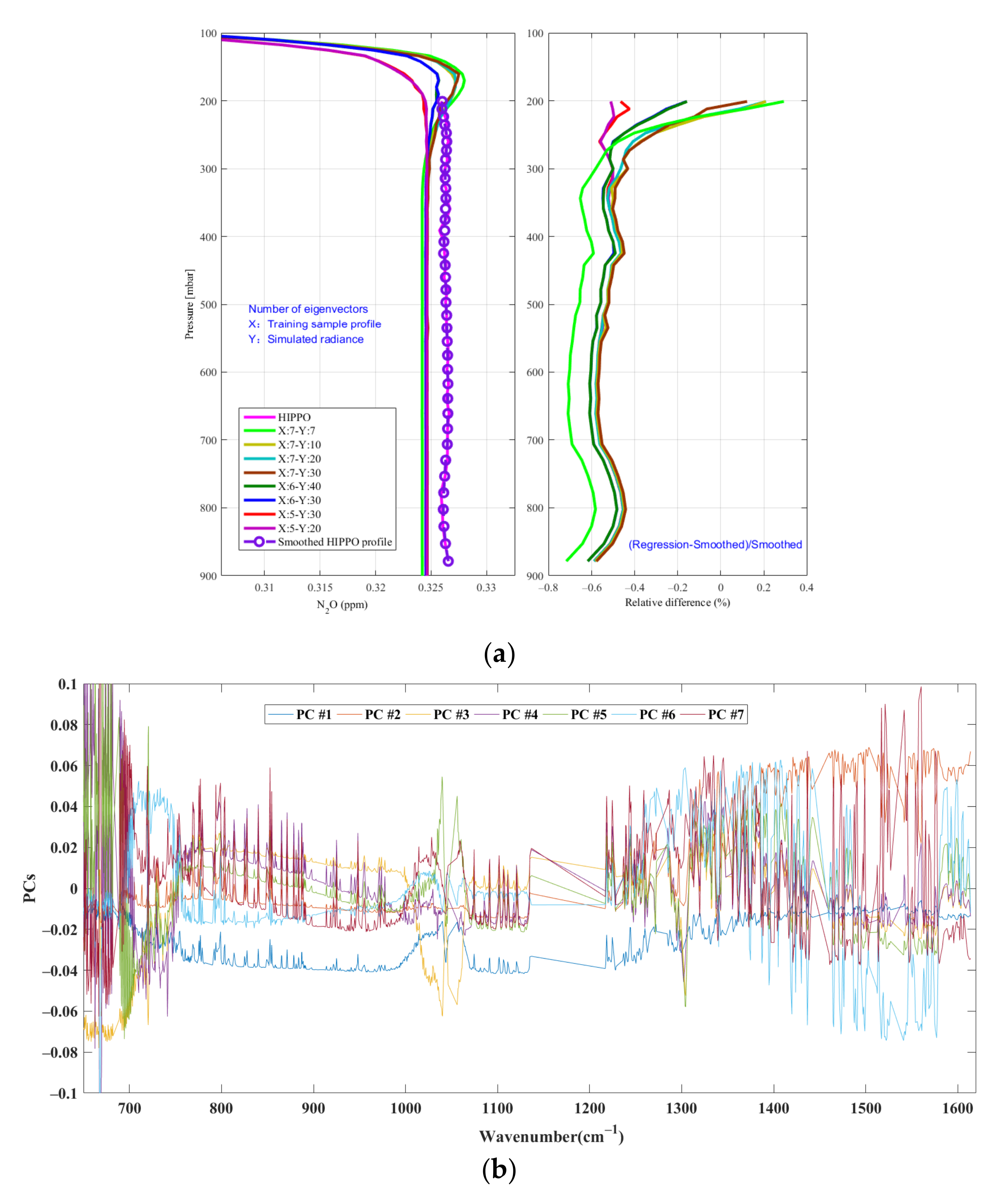
The statistical regression coefficients are calculated using different sets of eigenvectors, i.e., 5, 6, and 7 eigenvectors for the training samples, and 7, 10, 20, and 30 eigenvectors for the simulated BTs. Figure 1 shows the retrieval results obtained using various numbers of eigenvectors, as well as their relative difference (RD) from the High-Performance Instrumented Airborne Platform for Environmental Research (HIAPER) Pole-to-Pole Observations (HIPPO) data. The results show that the best accuracy is achieved with 5 eigenvectors for the training samples and 20 eigenvectors for the simulated BTs.
2.2. Channel Selection
The retrieval channel selection is one of the core issues for retrieval algorithms. Due to the sensor’s hyperspectral resolution, there are many spectral channels within the detection range. Since the retrieval using all channels needs a high computational cost, an optimal set of channels should be selected based on the target gas absorption, and the selected channels should contain the largest amount of information on the target gas but the least amount of information on interference gases [31]. In this section, based on the channel sensitivity, the spectral ranges within which the absorption of atmospheric N2O is the most intense and is not masked by the absorption of other gases (i.e., the spectral ranges within which N2O does not greatly overlap with other gases) are determined. In other words, the spectral ranges most sensitive to N2O are first identified. Then, based on the weighting functions, the channels that can help improve the retrieval accuracy and vertical resolution of the profiles are selected for retrieval.
Crevoisier et al. (2003) [32] proposed an optimal sensitivity profile (OSP) algorithm for AIRS data. The OSP algorithm classifies 2311 profiles in the Thermodynamic Initial Guess Retrieval (TIGR) dataset to 82 types of groups and eventually classifies these groups into three types, namely, tropical (28), mid-latitude (27), and polar (27). Each profile contains atmospheric temperature, humidity and O3 profiles and is divided into 40 layers. As proposed in Crevoisier et al. (2003) [32], the channel selection follows three principles: (1) when the radiance of the optimal channel for observing a certain gas is treated as “signal” and the interference from other gases is treated as “noise”, then channels with a relatively high SNR are selected; (2) when the signal of the observed gas is relatively small, the SNR may be relatively low—in this case, it is necessary to set a fixed signal threshold to remove the channel when the gas signal is smaller than the threshold; and (3) because the SNR is the integral of the whole atmosphere, the observation to some atmospheric pressure layers may not be possible if only using channels selected based on the SNR. Therefore, a Jacobian matrix is used to further select channels with various peaks.
Table 1 summarizes the N2O retrieval channels selected using the OSP algorithm. The OSP algorithm is unable to reflect the physical meanings of the channel selection and weighting functions. In this study, an improved OSP algorithm for channel selection (modified OSP) is proposed. First, the spectral ranges sensitive to N2O are determined considering the interference from other gases. Next, the transmittances of several main gases are calculated based on the AIRS data. In addition, channels with various transmittances that are unmasked by the transmittances of other trace gases are selected based on the spectral ranges determined in the first step. Finally, the weighting functions are approximately calculated from the re-derived equation (as described in Equation (8)) for weighting functions, and the channels with non-overlapping weighting function peaks are selected for retrieving atmospheric N2O profiles.
2.2.1. Analysis of Channel Sensitivity
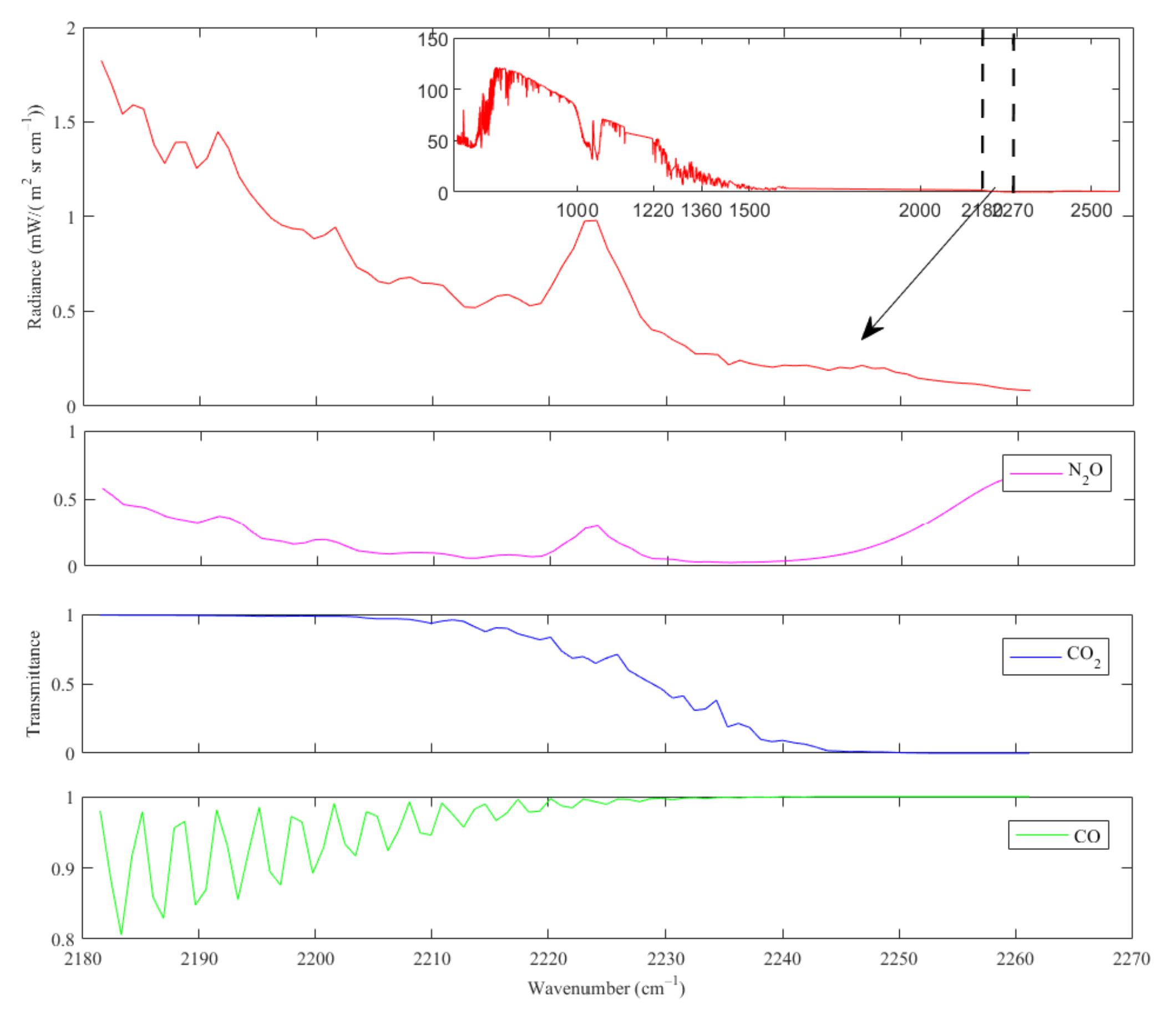
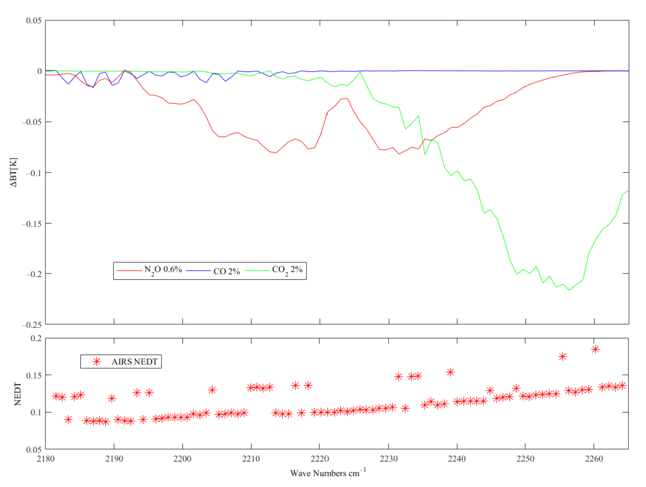
The three fundamental absorption features of N2O are centered at 1284.91 (υ1), 588.77 (υ2), and 2223.76 cm−1 (υ3). The υ1 band of N2O, the υ4 band (1310.76 cm−1) of CH4 and the main vibrational absorption band (1594.75 cm−1) of water vapor overlap one another. Consequently, it is very difficult to separate the absorption of N2O from CH4 and water vapor using the υ1 band of N2O. The υ2 band of N2O is outside the spectral range of AIRS and is thus not taken into consideration. Although the υ3 band of N2O is overlapped with part of the υ3 band of CO2 and part of the CO absorption band, the change in BT caused by the changes in CO2 (2%) and CO (2%) concentrations are much smaller than those caused by the change in N2O concentration. Figure 2 shows a segment of the AIRS spectrum near the υ1 absorption band of N2O, as well as the similar contributions of the two other major absorbing gases—water vapor and CH4 in this spectral range.
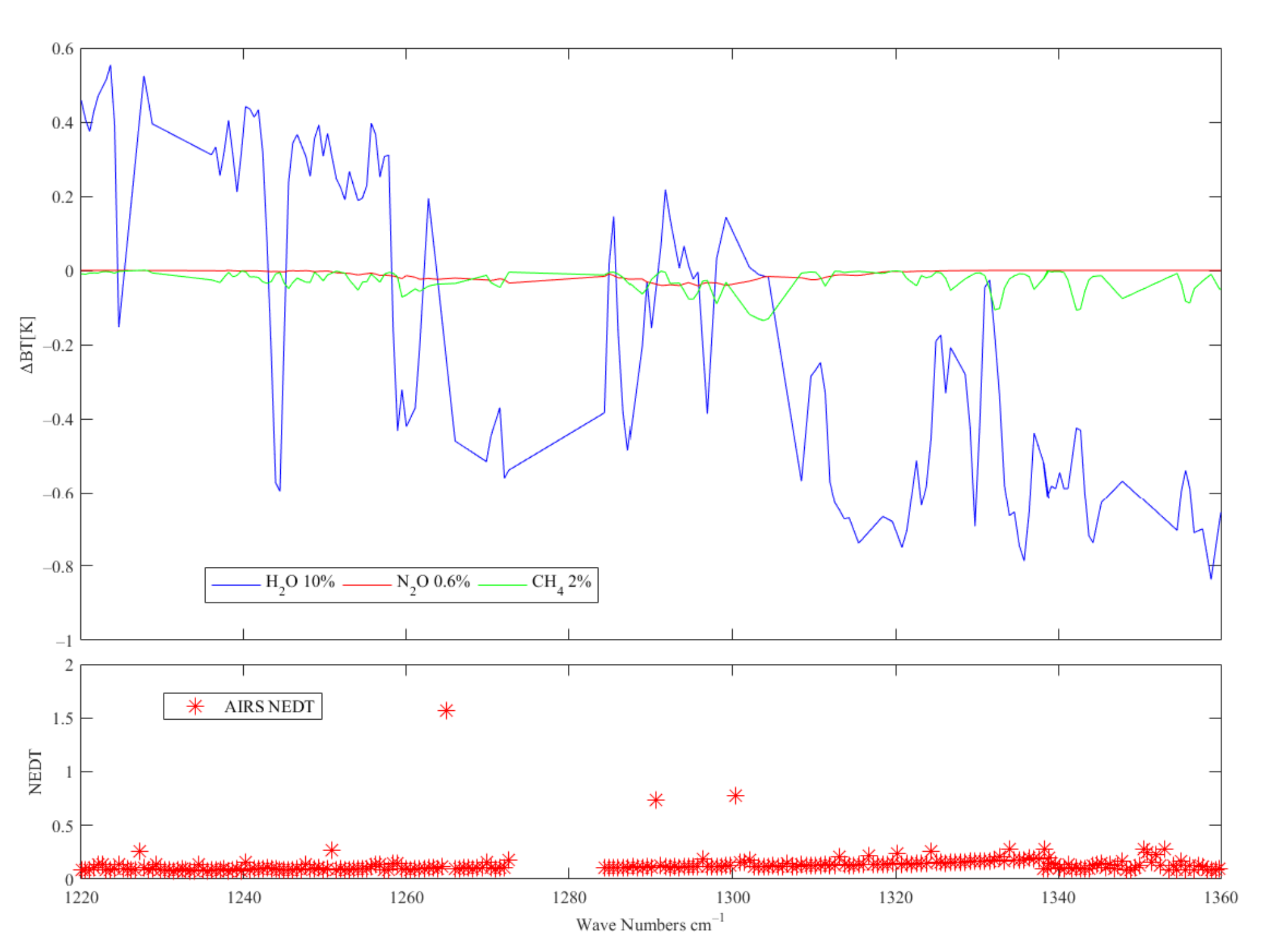
Figure 3 presented the changes in BTs caused by the changes in N2O, water vapor, and CH4 concentrations, the absorption band of N2O is overlapped with the absorption of CH4 and water vapor. Considering the AIRS channel noise [20], only two channels (at 1291.1395 and 1291.7086 cm−1) that are most sensitive to N2O but have less interference from other gases are selected, as marked in Figure 3. Using a similar method, some channels sensitive to N2O in υ3 band are selected, as shown in Figure 4 and Figure 5. This is the first step of channel selection.
2.2.2. Weighting Functions
Due to the correlations between the channels, a large number of retrieval channels is not necessarily favorable in the retrieval of atmospheric N2O profiles. Further selection based on weighting functions will be carried out. Without considering the surface contribution, the radiative transfer equation for the thermal IR region can be written in the form of the BT as below:
where T, z, and represent brightness temperatures, altitude, and transmittance, respectively. Most remote sensing problems and relevant retrieval algorithms can be simplified to Fredholm integral equations of the first kind [33], i.e.:
where is a kernel function; is the observed vector value, which is a known function, and is the function to be solved. Here, we assume that the average form ( and , the average value for and and let and . By subtracting the equation in the standard form from Equation (6) and then solving the first-order variation of the resultant equation [31], we have:
The kernel function (i.e., the weighting function) shows the sensitivity of the satellite observed radiance to the gas amounts as a function of the altitude.
As shown in Equation (6), the weighting function is essentially the convolution of atmospheric temperature and N2O transmittance profiles. The optimal information layer is located at the point of intersection between temperature and N2O profiles. Evidently, when the temperature profile remains unchanged, N2O concentrations at various altitudes can be determined by selecting channels with various transmittances. In this paper, the fast-forward CRTM is used to directly calculate the transmittances and weighting functions of several main gases affecting atmospheric N2O retrieval from the AIRS spectral channels.
Figure 6 shows the weighting functions of the two channels near the υ1 absorption band of N2O. The peak regions of the weighting functions of the two channels coincide with one another, and the weighting function of one channel exhibits larger peaks than that of the other channel. Therefore, only the channel with a larger peak is selected as the retrieval channel.
From the weighting functions of the channels selected near the υ3 absorption band of N2O, we noticed that most of the peaks overlap on each other. Only 13 channels with the largest peaks in various atmospheric pressure layers are selected for retrieval, as shown in Figure 7.
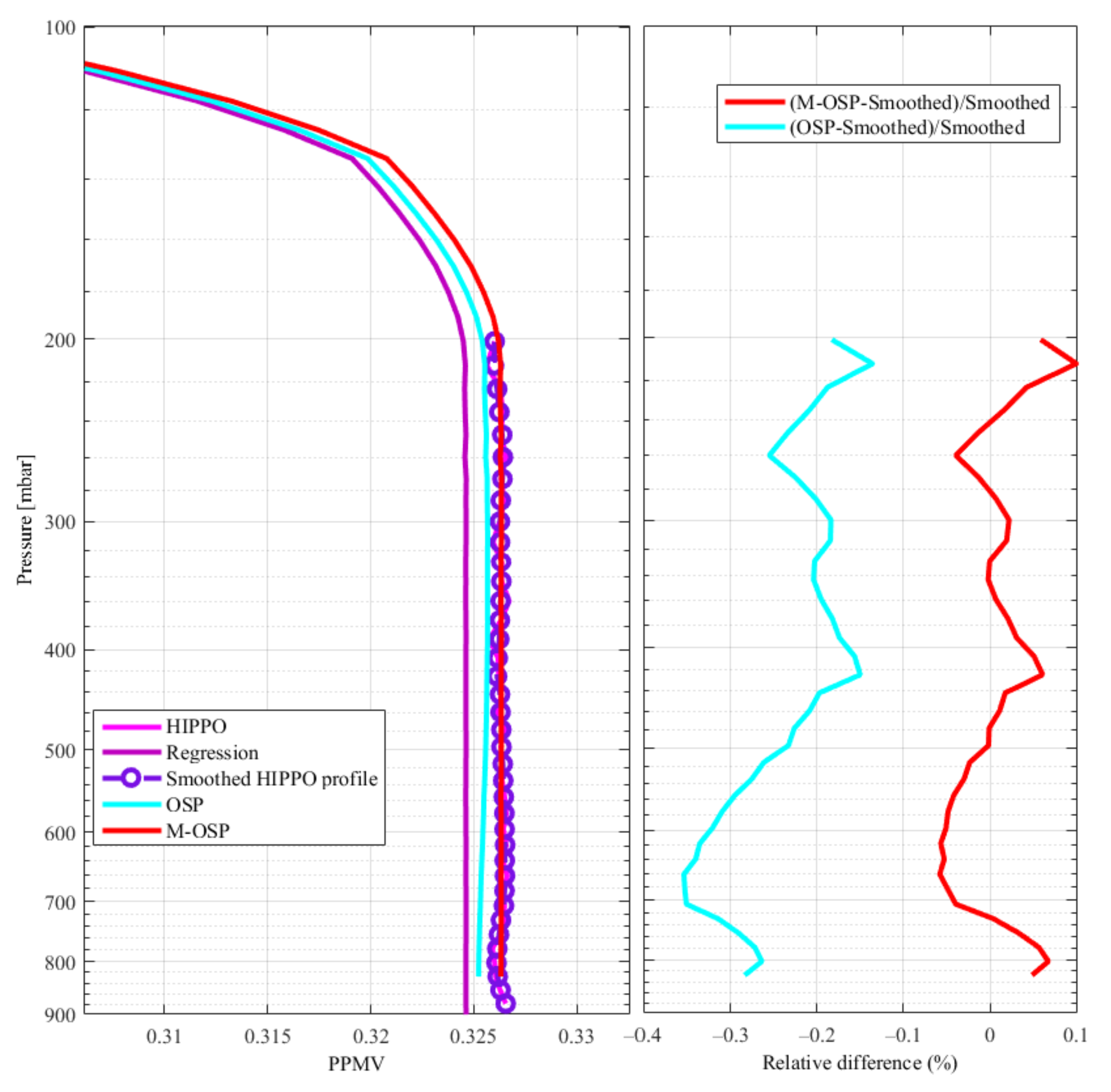
Table 2 shows the selected channels for N2O profile retrieval by the modified OSP method. Based on the weighting functions of the selected channels, AIRS is sensitive to N2O in the range of 200–800 hPa (i.e., the peak region of the weighting functions). Figure 8 shows the vertical atmospheric N2O profiles obtained using various channel selection algorithms. The retrieval run with the same setup as the M-OSP, with only difference being the retrieval channels. Evidently, the retrieval accuracy of the modified OSP algorithm proposed in this study is significantly higher than that of the OSP algorithm. The largest relative difference between the retrievals from the modified OSP algorithm and the HIPPO data is less than 0.1%.
3. Results and Discussion
The validation of results derived from satellite data is an essential step in improving retrieval algorithms, ensuring profile accuracy. In this study, atmospheric N2O profiles under clear-sky conditions were retrieved from AIRS Level-1B thermal IR radiance data. The retrieved profiles were validated using HIPPO N2O profile data and the data measured at the U.S. National Oceanic and Atmospheric Administration (NOAA)’s Earth System Research Laboratory (ESRL) observatories.
3.1. Validation Using HIPPO Observation Data
The HIPPO aircraft, supported by the U.S. NOAA and National Science Foundation, is used to observe greenhouse gases, trace gases with long lifespans, black carbon, and aerosols, as well as the carbon isotopic composition of CO2 [34]. The HIPPO aircraft flew five times across the Pacific Ocean from 85° N to 67° S, with vertical profiles approximately every 2.2° of latitude between 2009 and 2011. The fourth and fifth flights of the HIPPO aircraft, made between June and July 2011 and between August and September 2011, were used to validate the retrieval results (https://www.eol.ucar.edu/field_projects/hippo, accessed on 29 December 2022). During these missions, N2O is observed with a precision of 0.09 ppbv and an accuracy of 1.0 ppbv [35].
HIPPO data measured in the high-, mid-, and low-latitude regions of the Southern and Northern Hemispheres were selected to validate the algorithms. Table 3 lists the selected profiles. The match-up of AIRS with HIPPO measurements is selected if (1) the time difference is within 24 h and (2) the distance is within 100 km. Only the pixels with high-quality cloud-cleared radiance were used for retrieval.
Figure 9 shows the 13 retrievals matched up with HIPPO and the mean retrieval profile, and the RD between the retrieval results and the HIPPO data is shown in Figure 10. It is evident from Figure 10 that the retrieval comparisons are significantly improved when applying the averaging kernels to convolve the HIPPO data. The RD in layer 300–800 hPa is less than 0.1%, which demonstrates that AIRS is sensitive to N2O in the middle to upper troposphere, with the peak vertical sensitivity between 300–800 hPa.
Figure 11 shows the root-mean-square deviation (RMSD) and root-mean-square relative deviation (RMSRD) of the retrievals using all HIPPO data selected in Table 3. The RMSD is essentially less than 0.5 ppb and the RMSRD is less than 0.2%.
The retrieval accuracy is the highest for the range of 300–800 hPa and the RD is approximately 0.1% for nearly all the locations. The retrieval accuracy is lower for the range of 200–300 hPa and the lowest for values above 200 hPa.
Figure 12, Figure 13 and Figure 14 show examples of the retrieval results for regions at various latitudes. The retrieval results show that there is no significant difference between the atmospheric N2O profile concentrations in the troposphere over the high-latitude, mid-latitude, and tropical regions of the Southern Hemispheres. The retrieval accuracy is the highest for the range of 300–900 hPa and the lowest for values above 200 hPa. The largest RD exceeds 15%. In the thermal infrared (TIR), measurement sensitivity to the lowermost troposphere requires high thermal contrast between the Earth’s surface and the near-surface (tens to hundreds of meters above the surface) atmosphere. the reason for this retrieval accuracy over different altitude ranges might be associated with the lower thermal contrast. As shown in Figure 5, the averaging kernel is almost zero at surface 900 hpa, and the retrieved information almost entirely comes from the a priori.
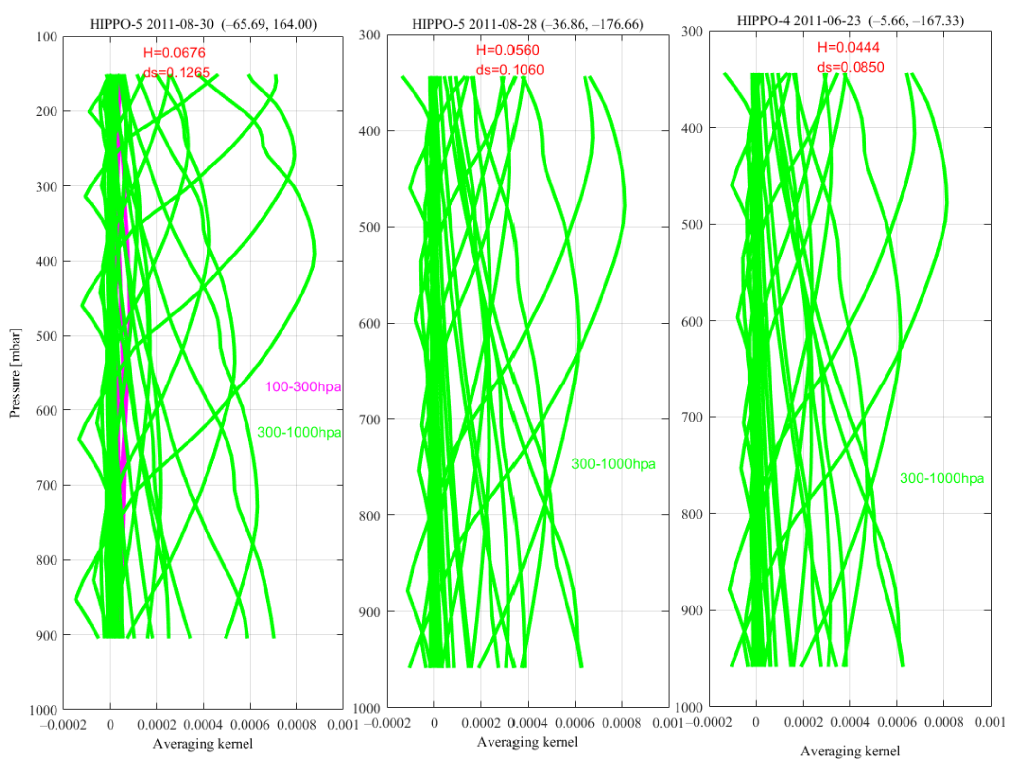
Figure 15 shows the sample AK matrices and the degree of freedom ds and entropy H for the AIRS observations over high-latitude, mid-latitude, and tropical regions. AK matrices characterize the sensitivity of the retrieved profiles relative to the true state of the atmosphere. These three measurements show different sensitivities at different latitudes to the N2O vertical distribution. The analysis reveals that the AIRS sensitivity to the N2O profile is greatest in the middle of troposphere (300–800 hPa). The information content and the degree of freedom are relatively low (ds = 0.0850), medium (ds = 0.1060), and high (ds = 0.1265). The ds is so low because it represents only what the second part of the retrieval brings as additional information that has limited room for improvement compared with the regression results. The value of the AKs from the surface to 900 hPa is close to zero.
3.2. Validation Using ESRL Observatory Data
Two research groups from the U.S. NOAA ESRL—the Halocarbons and Other Atmospheric Trace Species group and the Carbon Cycle Greenhouse Gases group—have been continuously observing N2O since 1977. Two sampling methods, in situ and flask, have been used. The flask method records near-surface monthly average measurements of N2O, whereas the in situ method records hourly, daily, monthly, and global measurements of N2O.
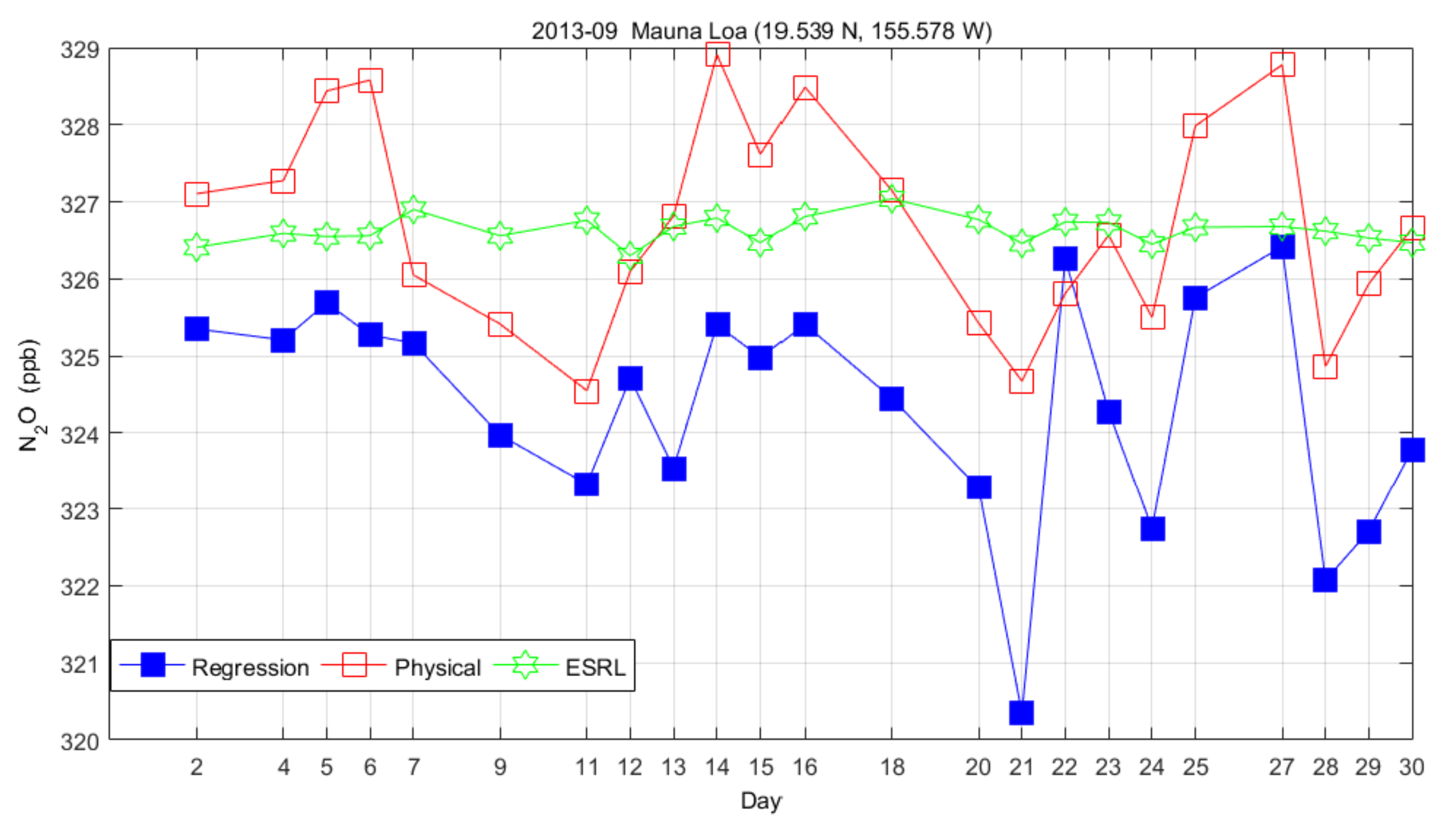
Data measured at the Mauna Loa Observatory (MLO) (coordinates: 19.539° N, 155.578° W; altitude: 3397 m) in Hawaii during 23 days of September 2013 available from the NOAA/ESRL Chromatograph for Atmospheric Trace Species (CATS) Program were selected and compared with the average satellite-observed values for all the matching points. The instrumental precision 5 of N2O is approximately 0.2% for NOAA CATS [36]. Observation points within a latitude range of 1° and a longitude range of 1° from the MLO were selected as matching points. The MLO is located at an altitude of 3.4 km. The value at a similar altitude (661 hPa) was selected for each matching point. Figure 16 shows the comparison.
The ESRL’s daily average data of N2O represent the average of all the hourly observations for each day (an observation is made each hour throughout the entire day (24 h)) and are thus relatively smooth. In comparison, each value retrieved from the AIRS data is the average of the values measured at the observation points matching the MLO at a certain time. As a result, a certain fluctuation (by 1–2 ppb) is observed in the values retrieved from the AIRS data. Overall, the values retrieved using the statistical regression algorithm are lower than the MLO observations.
4. Conclusions
One algorithm to retrieve atmospheric N2O profiles from AIRS data was presented, which includes the algorithm for a rapid initial profile retrieval and the channel selection under the framework of optimization theory. The channel selection was based on the physical meaning of this weighting function has been discussed in detail. Based on the weighting functions, as well as the transmittances of several main atmospheric gases and the sensitivity of their changes to BT, a total of 13 channels were selected for optimal retrieval in this paper. Theoretically, N2O concentrations in various atmospheric pressure layers can be retrieved if the channels with various transmittances of N2O can be located. However, in practice, channel selection faces challenges from widening satellite sounding channels and interference from other gases.
The retrieval results were validated using the profiles from HIPPO aircraft measurements and the ESRL data. The results show that this optimal estimation algorithm is more accurate than the statistical regression algorithm. The mean relative difference between the retrieved profiles and the HIPPO measurements is less than 0.1% in the vertical layers between 300–900 hPa. The retrieval accuracy is slightly lower in layers of 200–300 hPa (~5%) and the error is larger in layers above 200 hPa (>15%).
Because the absorption bands of N2O are mixed with other gases, future research will focus on simultaneous retrieval of the profiles of atmospheric temperatures, water vapor, and other gases that interfere N2O (e.g., CH4).
This study presents an algorithm for the retrieval of N2O profiles from the AIRS using a nonlinear optimal estimation method, although they are subject to limitations. For example, limited observation of sample points is available to verify the algorithm of the paper, and the results are limited to a specific time and area. More observations will be added to illustrate the reliability of the algorithm in the future.
Author Contributions
Conceptualization, P.M. and L.C.; data curation, C.Z.; methodology, C.C. and P.M.; supervision, S.Z. and Z.W.; validation, Y.Z. and L.Z.; writing—original draft, P.M. and C.C.; writing—review and editing, P.M. and C.C. All authors have read and agreed to the published version of the manuscript.
Funding
This research was funded by the National Natural Science Foundation of China (Grant No. 41501407), Key Special Project of “Inter-Government International Science and Technology Innovation Cooperation project” (Grant No. 2021YFE0117100) and the Major projects of high-resolution Earth observation system (Grant No. 05-Y30B01-9001-19/20-3).
Institutional Review Board Statement
Not applicable.
Informed Consent Statement
Not applicable.
Data Availability Statement
The data used to support the findings of this study are available from the corresponding authors upon reasonable request.
Conflicts of Interest
The authors declare no conflict of interest.
References
- IPCC. Climate Change 2013: The Physical Science Basis; Contribution of Working Group I to the Fifth Assessment Report of the Intergovernmental Panel on Climate Change; Cambridge University Press: Cambridge, UK, 2013. [Google Scholar]
- Montzka, S.A.; Dlugokencky, E.J.; Butler, J.H. Non-CO2 greenhouse gases and climate change. Nature 2011, 476, 43–50. [Google Scholar] [CrossRef] [PubMed]
- Ravishankara, A.R.; Daniel, J.S.; Portmann, R.W. Nitrous Oxide (N2O): The Dominant Ozone-Depleting Substance Emitted in the 21st Century. Science 2009, 326, 123–125. [Google Scholar] [CrossRef] [PubMed] [Green Version]
- Drummond, J.R.; Houghton, J.T.; Peskett, G.D.; Rodgers, C.D.; Wale, M.J.; Whitney, J.; Williamson, E.J. The stratospheric and mesospheric sounder on Nimbus 7. Philos. Trans. R. Soc. Lond. Ser. A Math. Phys. Sci. 1980, 296, 219–241. [Google Scholar]
- Urban, J.; Lautié, N.; Le Flochmoën, E.; Jiménez, C.; Eriksson, P.; De La Noë, J.; Dupuy, E.; El Amraoui, L.; Frisk, U.; Jégou, F.; et al. Odin/SMR limb observations of stratospheric trace gases: Validation of N2O. J. Geophys. Res. Atmos. 2005, 110, D09301. [Google Scholar] [CrossRef] [Green Version]
- Lambert, A.; Read, W.G.; Livesey, N.J.; Santee, M.L.; Manney, G.L.; Froidevaux, L.; Wu, D.L.; Schwartz, M.J.; Pumphrey, H.C.; Jimenez, C.; et al. Validation of the Aura Microwave Limb Sounder middle atmosphere water vapor and nitrous oxide measurements. J. Geophys. Res. Atmos. 2007, 112, D24S36. [Google Scholar] [CrossRef]
- Camy-Peyret, C.; Dufour, G.; Payan, S.; Oelhaf, H.; Wetzel, G.; Stiller, G.; Blumenstock, T.; Blom, C.E.; Gulde, T.; Glatthor, N.; et al. Validation of MIPAS N2O profiles by stratospheric balloon, aircraft and ground based measurements. In Proceedings of the Second Workshop on the Atmospheric Chemistry Validation of Envisat (ACVE-2), Frascati, Italy, 3–7 May 2004. ESA Special Publication SP-562, August 2004. [Google Scholar]
- Strong, K.; Wolff, M.A.; Kerzenmacher, T.E.; Walker, K.A.; Bernath, P.F.; Blumenstock, T.; Boone, C.; Catoire, V.; Coffey, M.; De Mazière, M.; et al. Validation of ACE-FTS N2O measurements. Atmos. Chem. Phys. 2008, 8, 4759–4786. [Google Scholar] [CrossRef] [Green Version]
- Gunson, M.R.; Abbas, M.M.; Abrams, M.C.; Allen, M.; Brown, L.R.; Brown, T.L.; Chang, A.Y.; Goldman, A.; Irion, F.W.; Lowes, L.L.; et al. The Atmospheric Trace Molecule Spectroscopy (ATMOS) experiment: Deployment on the ATLAS space shuttle missions. Geophys. Res. Lett. 1996, 23, 2333–2336. [Google Scholar] [CrossRef] [Green Version]
- Irion, F.W.; Gunson, M.R.; Toon, G.C.; Chang, A.Y.; Eldering, A.; Mahieu, E.; Manney, G.L.; Michelsen, H.A.; Moyer, E.J.; Newchurch, M.J.; et al. Atmospheric Trace Molecule Spectroscopy (ATMOS) Experiment Version 3 data retrievals. Appl. Opt. 2002, 41, 6968–6979. [Google Scholar] [CrossRef] [Green Version]
- Nakajima, H.; Sugita, T.; Yokota, T.; Sasano, Y. Atmospheric environment monitoring by the ILAS-II onboard the ADEOS-II satellite. Proc. SPIE 2004, 5571, 293–300. [Google Scholar]
- Xiong, X.; Maddy, E.S.; Barnet, C.; Gambacorta, A.; Patra, P.K.; Sun, F.; Goldberg, M. Retrieval of nitrous oxide from Atmospheric Infrared Sounder: Characterization and validation. J. Geophys. Res. Atmos. 2014, 119, 9107–9122. [Google Scholar] [CrossRef]
- Worden, J.; Kulawik, S.; Frankenberg, C.; Payne, V.; Bowman, K.; Cady-Peirara, K.; Wecht, K.; Lee, J.-E.; Noone, D. Profiles of CH4, HDO, H2O, and N2O with improved lower tropospheric vertical resolution from Aura TES radiances. Atmos. Meas. Tech. 2012, 5, 397–411. [Google Scholar] [CrossRef] [Green Version]
- Clerbaux, C.; Boynard, A.; Clarisse, L.; George, M.; Hadji-Lazaro, J.; Herbin, H.; Hurtmans, D.; Pommier, M.; Razavi, A.; Turquety, S.; et al. Monitoring of atmospheric composition using the thermal infrared IASI/MetOp sounder. Atmos. Chem. Phys. 2009, 9, 6041–6054. [Google Scholar] [CrossRef] [Green Version]
- Bloom, H.J. The Cross-track Infrared Sounder (CrIS): A sensor for operational meteorological remote sensing. In Proceedings of the IGARSS 2001. Scanning the Present and Resolving the Future. IEEE 2001 International Geoscience and Remote Sensing Symposium (Cat. No. 01CH37217), Sydney, NSW, Australia, 9–13 July 2001; IEEE: Piscataway, NJ, USA, 2001; Volume 3, pp. 1341–1343. [Google Scholar]
- Aumann, H.H.; Chahine, M.T.; Gautier, C.; Goldberg, M.D.; Kalnay, E.; McMillin, L.M.; Revercomb, H.; Rosenkranz, P.W.; Smith, W.L.; Staelin, D.H.; et al. AIRS/AMSU/HSB on the Aqua mission: Design, science objectives, data products, and processing systems. IEEE Trans. Geosci. Remote Sens. 2003, 41, 253–264. [Google Scholar] [CrossRef] [Green Version]
- Ma, P.-F.; Xiong, X.-Z.; Chen, L.F.; Tao, M.-H.; Chen, H.; Zhang, Y.-H.; Zhang, L.-J.; Li, Q.; Zhou, C.-Y.; Chen, C.-H.; et al. Temporal and Spatial Characteristics of Nitrous Oxide Concentration in China. Spectrosc. Spectr. Anal. 2021, 41, 20–24. [Google Scholar]
- Rodgers, C.D. Inverse Methods for Atmospheric Sounding: Theory and Practice; World Scientific Publishing: Singapore, 2008; 240p. [Google Scholar]
- Petropavlovskikh, I.; Bhartia, P.K.; DeLuisi, J. An Improved Umkehr Algorithm; NOAA Cooperative Institute for Research in Environmental Sciences: Boulder, CO, USA, 2004. [Google Scholar]
- Barnet, C.D.; Goldberg, M.D.; McMillin, L.; Chahine, M.T. Remote sounding of trace gases with the EOS/AIRS instrument. In Atmospheric and Environmental Remote Sensing Data Processing and Utilization: An End-to-End System Perspective; SPIE: Bellingham, WA, USA, 2004; p. 5548. [Google Scholar] [CrossRef]
- Eyre, J. Inversion Methods for Satellite Sounding Data. ECMWF Meteorological Training Course Lecture Series. 2002. Available online: https://www.ecmwf.int/node/16942 (accessed on 8 April 2022).
- Chen, L.F.; Liu, Q.H.; Li, Z.L.; Xu, X.R. The couple-inversion of atmospheric profile and surface temperature and emissivity from MODIS data. In IEEE International Geoscience and Remote Sensing Symposium; IEEE: Piscataway, NJ, USA, 2002; Volume 3, pp. 1630–1632. [Google Scholar]
- Han, Y.; van Delst, P.; Liu, Q.H.; Weng, F.Z.; Yan, B.H.; Treadon, R.; Derber, J. JCSDA Community Radiative Transfer Model (CRTM)—Version 1, NOAA Tech. Rep. NESDIS 122. 2006. Available online: https://repository.library.noaa.gov/view/noaa/1157 (accessed on 8 April 2022).
- Goldberg, M.D.; Qu, Y.; McMillin, L.M.; Wolf, W.; Zhou, L.; Divakarla, M. AIRS near-real-time products and algorithms in support of operational numerical weather prediction. IEEE Trans. Geosci. Remote Sens. 2003, 41, 379–389. [Google Scholar] [CrossRef]
- Susskind, J.; Barnet, C.; Blaisdell, J. Retrieval of atmospheric and surface parameters from AIRS/AMSU/HSB data in the presence of clouds. IEEE Trans. Geosci. Remote Sens. 2003, 41, 309–409. [Google Scholar] [CrossRef]
- Matricardi, M. The Generation of RTTOV Regression Coefficients for IASI and AIRS Using a New Profile Training Set and a New Lineby-line Database; ECMWF Research Dept. Tech. Memo.; European Centre for Medium Range Weather Forecasts: Berkshire, UK, 2008; p. 564. Available online: http://www.ecmwf.int/publications (accessed on 29 December 2021).
- Chevallier, F.; Di Michele, S.; McNally, A.P. Diverse Profile Datasets from the ECMWF 91-Level Short-Range Forecasts, NWP SAF Report No. NWPSAF-EC-TR-010. 2006. Available online: https://www.ecmwf.int/en/elibrary/8685-diverse-profile-datasets-ecmwf-91-level-short-range-forecasts (accessed on 8 April 2022).
- Smith, W.L.; Woolf, H.M. The use of eigenvectors of statistical covariance matrices for interpreting satellite sounding radiometer observations. J. Atmos. Sci. 1976, 33, 1127–1140. [Google Scholar] [CrossRef] [Green Version]
- Smith, W.L.; Weisz, E.; Kireev, S.V.; Zhou, D.K.; Li, Z.; Borbas, E.E. Dual-Regression Retrieval Algorithm for Real-Time Processing of Satellite Ultraspectral Radiances. J. Appl. Meteorol. Climatol. 2012, 51, 1455–1476. [Google Scholar] [CrossRef]
- Ma, P.F.; Chen, L.F.; Li, Q.; Tao, M.H.; Wang, Z.F.; Zhang, Y.; Zhong-Ting, W.; Zhou, C.Y. Simulation of Atmospheric Nitrous Oxide Profiles Retrieval from AIRS Observations. Spectrosc. Spectr. Anal. 2015, 35, 1690–1694. [Google Scholar]
- Zeng, Q.C. Principles for Atmospheric Infrared Remote Sensing; Science Press: Beijing, China, 1974. [Google Scholar]
- Crevoisier, C.; Chedin, A.; Scott, N.A. AIRS channel selection for CO2 and other trace gas retrievals. Q. J. R. Meteorol. Soc. 2003, 129, 2719–2740. [Google Scholar] [CrossRef]
- Fredholm, I. Sur une classe d’équations fonctionnelles. Acta Math. 1903, 27, 365–390. [Google Scholar] [CrossRef]
- Wofsy, S.C. HIAPER Pole-to-Pole Observations (HIPPO): Fine-grained, global-scale measurements of climatically important atmospheric gases and aerosols. Philos. Trans. R. Soc. A Math. Phys. Eng. Sci. 2011, 369, 2073–2086. [Google Scholar] [CrossRef]
- Santoni, G.W.; Daube, B.C.; Kort, E.A.; Jiménez, R.; Park, S.; Pittman, J.V.; Gottlieb, E.; Xiang, B.; Zahniser, M.S.; Nelson, D.D.; et al. Evaluation of the airborne quantum cascade laser spectrometer (QCLS) measurements of the carbon and greenhouse gas suite–CO2, CH4, N2O, and CO–during the CalNex and HIPPO campaigns. Atmos. Meas. Tech. 2014, 7, 1509–1526. [Google Scholar] [CrossRef] [Green Version]
- Saikawa, E.; Prinn, R.G.; Dlugokencky, E.; Ishijima, K.; Dutton, G.S.; Hall, B.D.; Langenfelds, R.; Tohjima, Y.; Machida, T.; Manizza, M.; et al. Global and regional emissions estimates for N2O. Atmos. Chem. Phys. 2014, 14, 4617–4641. [Google Scholar] [CrossRef] [Green Version]
Figure 1.
Statistical regression results and seven eigenvectors for simulated BTs. (a) Statistical regression results obtained using various numbers of eigenvectors and their relative difference from HIPPO measurement data (time: 10 June 2011). (b) Eigenvectors for simulated BTs (in order to draw the continuous line segments, here only part of the bands (650–1620 cm−1) were selected).

Figure 2.
A segment of the AIRS spectrum near the υ1 absorption band of N2O (top plot) and the transmittances of N2O, water vapor and CH4 (bottom three plots) in the MWIR range.
Figure 2.
A segment of the AIRS spectrum near the υ1 absorption band of N2O (top plot) and the transmittances of N2O, water vapor and CH4 (bottom three plots) in the MWIR range.

Figure 3.
Changes in the BT near the υ1 absorption band of N2O that occur when the water vapor, N2O and CH4 concentrations increase by 10%, 0.6%, and 2%, respectively, (top) and the AIRS channel noise in the υ1 absorption band of N2O (bottom).
Figure 3.
Changes in the BT near the υ1 absorption band of N2O that occur when the water vapor, N2O and CH4 concentrations increase by 10%, 0.6%, and 2%, respectively, (top) and the AIRS channel noise in the υ1 absorption band of N2O (bottom).

Figure 4.
A segment of the AIRS spectrum near the υ3 absorption band of N2O (top plot) and the transmittances of N2O, CO2, and CO (bottom three plots) in the SIR range.
Figure 4.
A segment of the AIRS spectrum near the υ3 absorption band of N2O (top plot) and the transmittances of N2O, CO2, and CO (bottom three plots) in the SIR range.

Figure 5.
Changes in BT near the υ3 absorption band of N2O that occur when the CO2, N2O, and CO concentrations increase by 2%, 0.6%, and 2%, respectively, (top) and AIRS channel noise in the υ3 absorption band of N2O (bottom).
Figure 5.
Changes in BT near the υ3 absorption band of N2O that occur when the CO2, N2O, and CO concentrations increase by 2%, 0.6%, and 2%, respectively, (top) and AIRS channel noise in the υ3 absorption band of N2O (bottom).

Figure 6.
Weighting functions of the channels selected near the υ1 absorption band of N2O.

Figure 7.
Weighting functions of all the channels selected for retrieval.

Figure 8.
N2O profiles retrieved using various channel selection algorithms (time: 10 June 2011).

Figure 9.
An example of the retrieval results for the mid-latitude region of the Northern Hemisphere.
Figure 9.
An example of the retrieval results for the mid-latitude region of the Northern Hemisphere.

Figure 10.
Average retrieval results for the 13 sample points matching the HIPPO data (left) and the RD between the retrieval results and the HIPPO data (right).
Figure 10.
Average retrieval results for the 13 sample points matching the HIPPO data (left) and the RD between the retrieval results and the HIPPO data (right).

Figure 11.
The root-mean-square deviation (RMSD) and root-mean-square RD (RMSRD) of the retrievals using all HIPPO data selected in Table 3.
Figure 11.
The root-mean-square deviation (RMSD) and root-mean-square RD (RMSRD) of the retrievals using all HIPPO data selected in Table 3.

Figure 12.
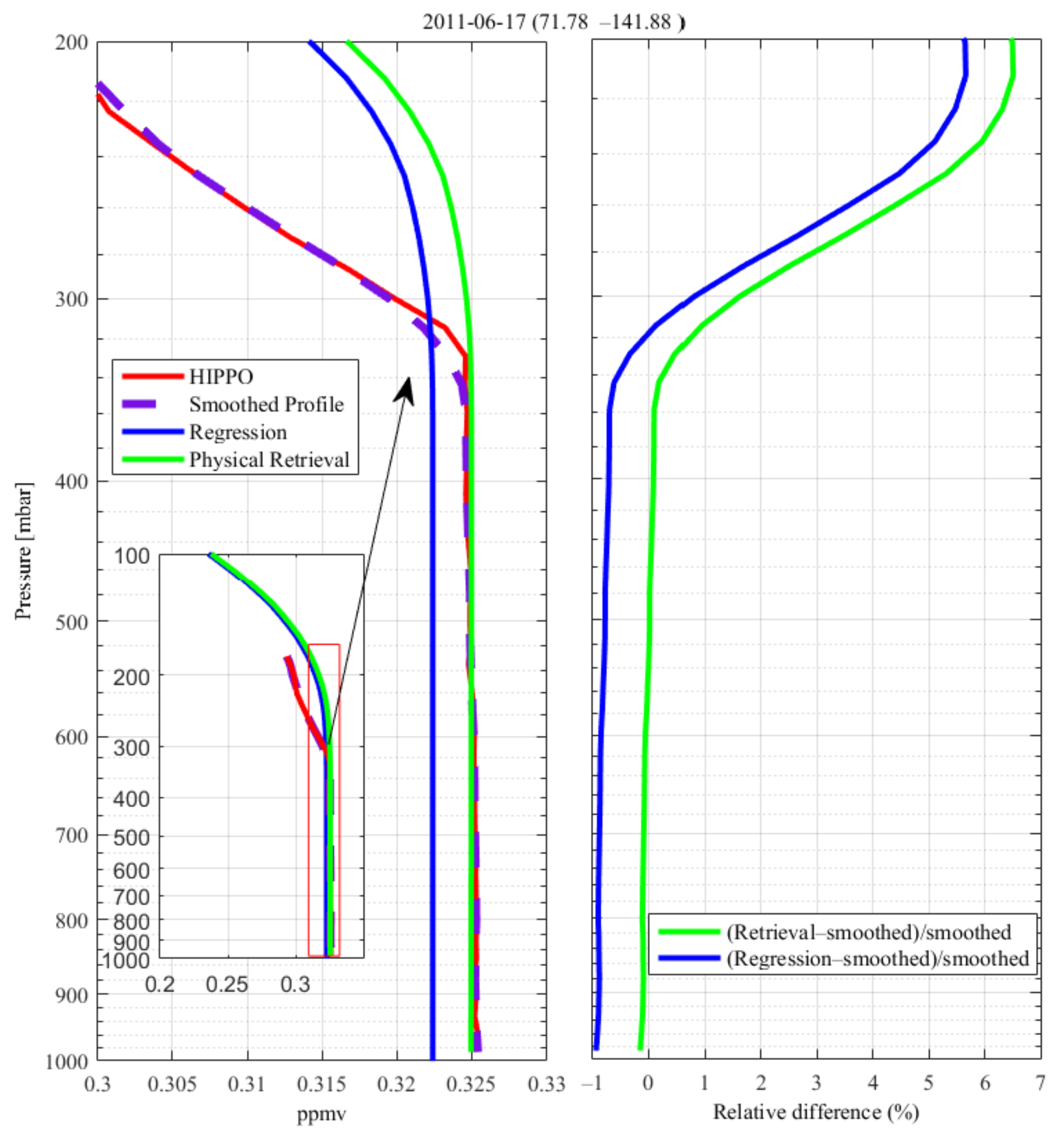
An example of the retrieval results for the high-latitude region of the Northern Hemisphere (left) and the RD between the retrieval results and the HIPPO data (right).
Figure 12.
An example of the retrieval results for the high-latitude region of the Northern Hemisphere (left) and the RD between the retrieval results and the HIPPO data (right).

Figure 13.
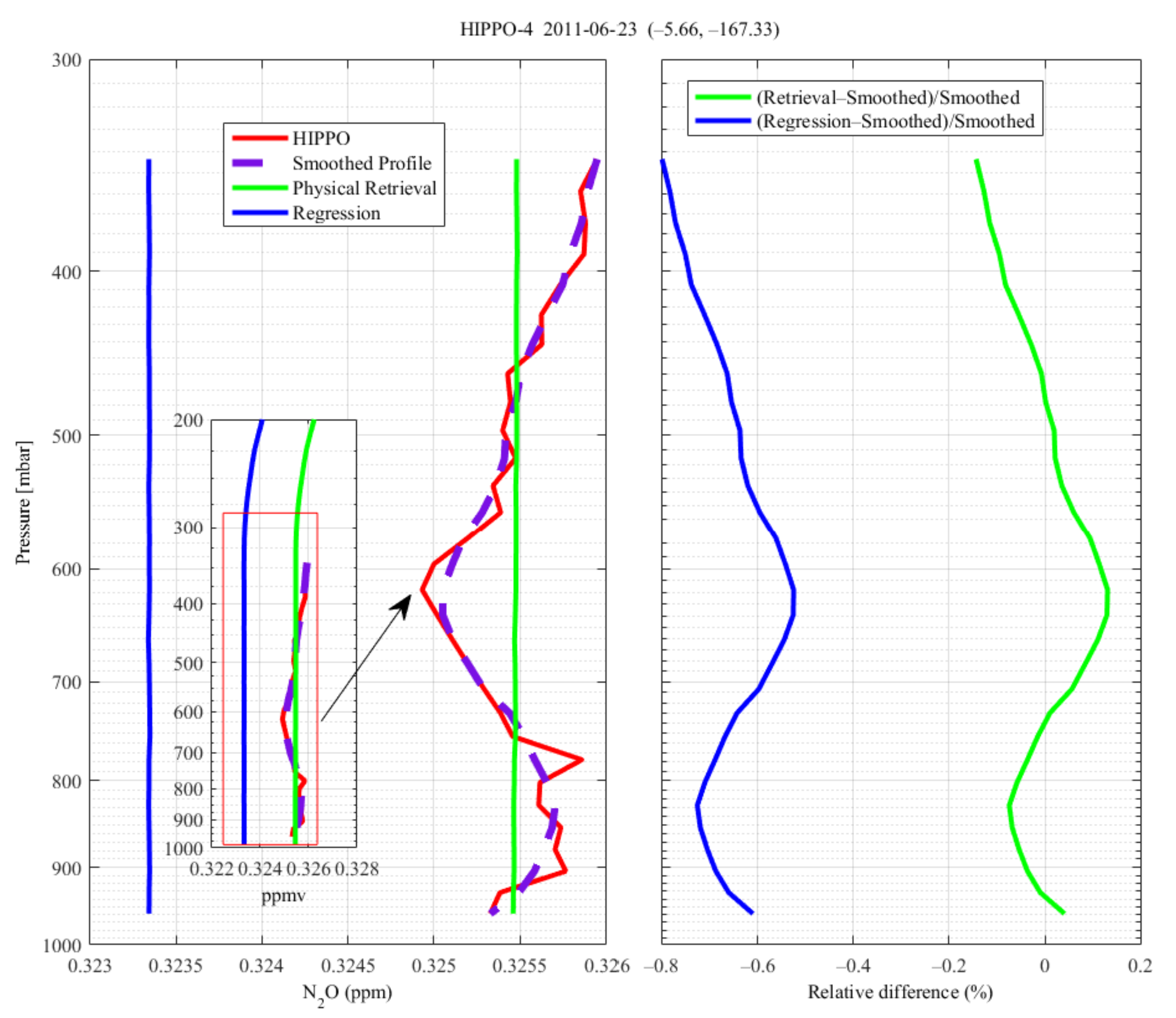
An example of the retrieval results for the tropical region (left) and the RD between the retrieval results and the HIPPO data (right).
Figure 13.
An example of the retrieval results for the tropical region (left) and the RD between the retrieval results and the HIPPO data (right).

Figure 14.
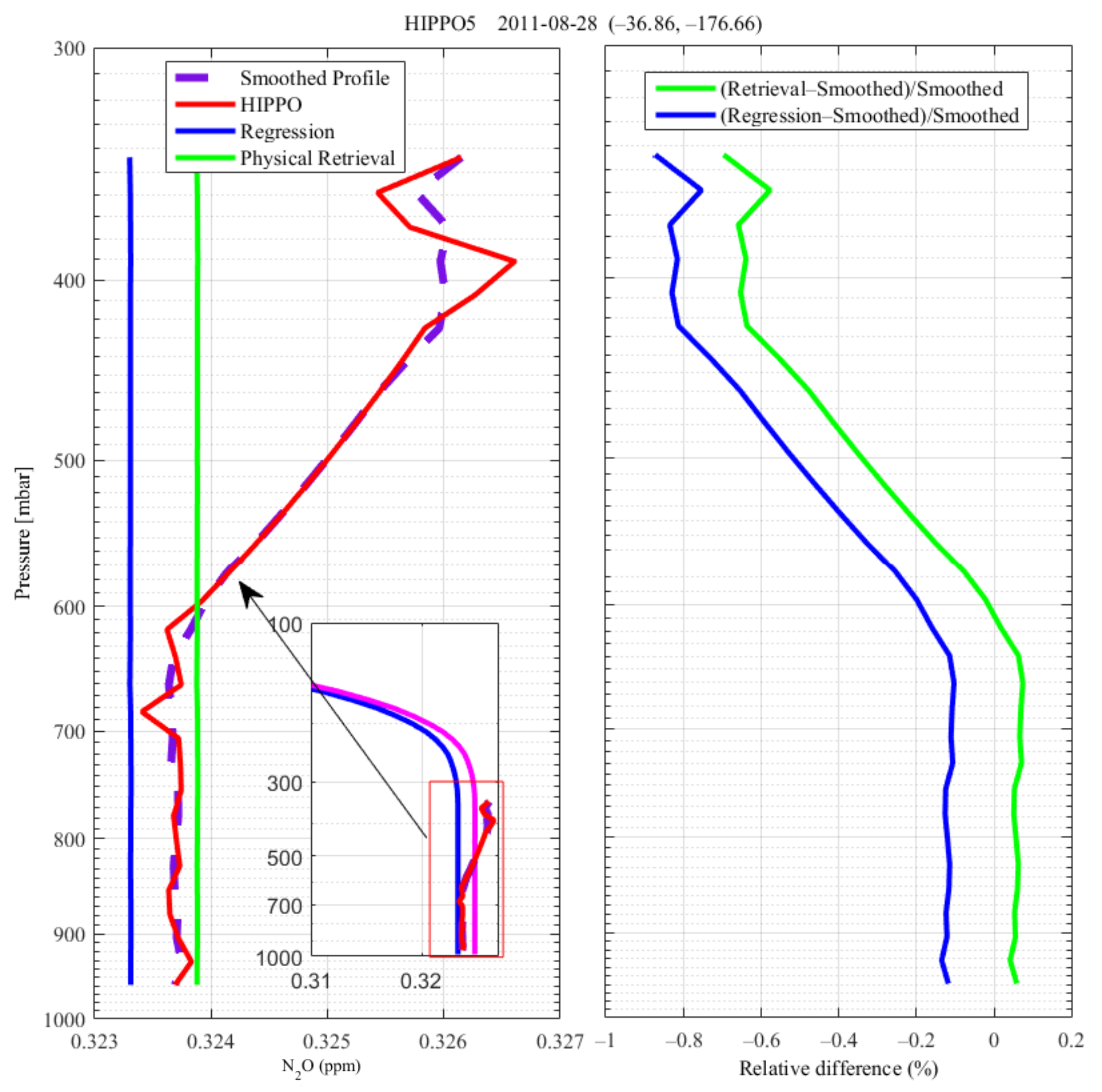
An example of the retrieval results for the mid-latitude region of the Southern Hemisphere (left) and the RD between the retrieval results and the HIPPO data (right).
Figure 14.
An example of the retrieval results for the mid-latitude region of the Southern Hemisphere (left) and the RD between the retrieval results and the HIPPO data (right).

Figure 15.
Examples of AKs for the measurements over tropical (left), mid-latitude (middle), and high-latitude (right) regions.
Figure 15.
Examples of AKs for the measurements over tropical (left), mid-latitude (middle), and high-latitude (right) regions.

Figure 16.
Comparison of the results retrieved from the AIRS data and the MLO observations for September 2013.
Figure 16.
Comparison of the results retrieved from the AIRS data and the MLO observations for September 2013.


Table 1.
The selected AIRS channels number for N2O retrieval using the OSP algorithm.
| Number of AIRS Channels | Wavenumber (cm−1) |
|---|---|
| 1883 | 2197.91 |
| 1884 | 2198.83 |
| 1897 | 2210.85 |
| 1901 | 2214.57 |
| 1917 | 2229.59 |
| 1921 | 2233.38 |
| 1923 | 2235.27 |
| 1924 | 2236.22 |
Table 2.
The selected channels for N2O retrieval using the modified OSP algorithm.
| Number of AIRS Channels | Wavenumber (cm−1) |
|---|---|
| 1382 | 1291.7086 |
| 1883 | 2197.9108 |
| 1898 | 2211.7779 |
| 1900 | 2213.6399 |
| 1916 | 2228.6466 |
| 1919 | 2231.4825 |
| 1920 | 2232.4294 |
| 1924 | 2236.2248 |
| 1925 | 2237.1756 |
| 1926 | 2238.1272 |
| 1927 | 2239.0796 |
| 1929 | 2240.9868 |
| 1930 | 2241.9415 |
Table 3.
HIPPO data selected to validate the algorithms.
| HIPPO (Flight Number) | Time | Latitude | Longitude | |
|---|---|---|---|---|
| 1 | 4 | 10 June 2011 | 32.63 | −103.14 |
| 2 | 4 | 17 June 2011 | 71.78 | −141.88 |
| 3 | 4 | 23 June 2011 | −5.66 | −167.33 |
| 4 | 5 | 28 August 2011 | −36.86 | 176.66 |
| 5 | 5 | 30 August 2011 | −65.69 | 164.00 |
Publisher’s Note: MDPI stays neutral with regard to jurisdictional claims in published maps and institutional affiliations. |
© 2022 by the authors. Licensee MDPI, Basel, Switzerland. This article is an open access article distributed under the terms and conditions of the Creative Commons Attribution (CC BY) license (https://creativecommons.org/licenses/by/4.0/).
Share and Cite
MDPI and ACS Style
Chen, C.; Ma, P.; Chen, L.; Zhang, Y.; Zhou, C.; Zhao, S.; Zhang, L.; Wang, Z. Nitrous Oxide Profile Retrievals from Atmospheric Infrared Sounder and Validation. Atmosphere 2022, 13, 619. https://doi.org/10.3390/atmos13040619
AMA Style
Chen C, Ma P, Chen L, Zhang Y, Zhou C, Zhao S, Zhang L, Wang Z. Nitrous Oxide Profile Retrievals from Atmospheric Infrared Sounder and Validation. Atmosphere. 2022; 13(4):619. https://doi.org/10.3390/atmos13040619
Chicago/Turabian StyleChen, Cuihong, Pengfei Ma, Liangfu Chen, Yuhuan Zhang, Chunyan Zhou, Shaohua Zhao, Lianhua Zhang, and Zhongting Wang. 2022. "Nitrous Oxide Profile Retrievals from Atmospheric Infrared Sounder and Validation" Atmosphere 13, no. 4: 619. https://doi.org/10.3390/atmos13040619
Note that from the first issue of 2016, this journal uses article numbers instead of page numbers. See further details here.