
Observed Relationship between Ozone and Temperature for Urban Nonattainment Areas in the United States


School of Science, Technology, Engineering and Mathematics, University of Washington Bothell, 18115 Campus Way NE, Bothell, WA 98011, USA
*
Author to whom correspondence should be addressed.
Atmosphere 2021, 12(10), 1235; https://doi.org/10.3390/atmos12101235
Submission received: 29 August 2021
/
Revised: 16 September 2021
/
Accepted: 20 September 2021
/
Published: 22 September 2021
(This article belongs to the Section Climatology)
Abstract
:This study examined the observed relationship between ozone (O3) and temperature using data from 1995 to 2020 at 20 cities across the United States (U.S.) that exceed the O3 National Ambient Air Quality Standard (NAAQS). The median slope of the O3 versus temperature relationship decreased from 2.8 to 1.5 parts per billion per degrees Celsius (ppb °C−1) in the eastern U.S., 2.2 to 1.3 ppb °C−1 in the midwestern U.S., and 1.7 to 1.1 ppb °C−1 in the western U.S. O3 in the eastern and midwestern U.S. has become less correlated with temperature due to emission controls. In the western U.S., O3 concentrations have declined more slowly and the correlation between O3 and temperature has changed negligibly due to the effects of high background O3 and wildfire smoke. This implies that meeting the O3 NAAQS in the western U.S. will be more challenging compared with other parts of the country.
1. Introduction
Tropospheric ozone (O3) is an important oxidant that is detrimental to human health and welfare at high concentrations [1,2,3]. O3 is formed due to photochemical reactions between oxides of nitrogen (NOx = NO + NO2) and volatile organic compounds (VOCs). Over the past few decades, most regions of the United States (U.S.) have significantly reduced anthropogenic NOx and VOC emissions [4]. As a result, peak O3 levels have substantially decreased across much of the U.S. [5,6,7]. In 2015, the U.S. Environmental Protection Agency (EPA) lowered the O3 National Ambient Air Quality Standard (NAAQS) to 70 parts per billion (ppb) [8]. The standard is met when the annual fourth-highest maximum daily 8-h average (MDA8) O3 concentration is 70 ppb or less, averaged over a three-year period. Areas that are not in compliance with the O3 NAAQS are designated as nonattainment areas (NAAs) [9]. For NAAs, it is essential to have a detailed understanding of the chemical and meteorological processes influencing O3 formation so that appropriate pollution control strategies can be created to achieve compliance with the O3 NAAQS.
The meteorological conditions that are conducive to photochemical O3 production are high temperature, abundant solar radiation, low relative humidity, and low wind speed [10,11,12]. In most continental environments, the relationship between summertime O3 and temperature is approximately linear. Calculating the slope of the O3 versus temperature relationship (mO3-T) is one way to assess the dependence of O3 on temperature.
Previous work has defined mO3-T as the slope of either the MDA8 O3 versus the daily maximum temperature (TMAX) or the hourly O3 versus the hourly temperature. Values of mO3-T have been called the “climate penalty,” indicating that sufficiently stringent emission reductions of O3 precursors will be necessary to offset the impacts of increasing surface temperatures [13,14]. Many previous studies have reported observed and/or modeled mO3-T values ranging from approximately 0 to 11.3 ppb °C−1 for rural and/or urban locations throughout the U.S. [7,13,15,16,17,18,19,20,21,22,23,24,25]. Higher mO3-T values were typically found for urban areas, consistent with O3 production being more sensitive to temperature in NOx-saturated environments [26].
Even though mO3-T values have been widely reported, no previous studies have examined the long-term relationship between O3 and temperature for urban NAAs throughout the U.S. This gap is noteworthy for two reasons. First, the summertime O3 production regime in many U.S. cities has become more sensitive to NOx due to ongoing NOx emission reductions [27,28]. Second, since 1970, global-average land temperatures have increased by approximately 1.5 °C or 0.3 °C per decade [29]. For these reasons, it is likely that the current dependence of O3 on temperature differs compared with the 1990s and early 2000s.
This study investigated the observed relationship between O3 and temperature for a group of urban NAAs in the U.S. from 1995 to 2020. The 20 urban NAAs considered in this study were in O3 nonattainment for the full analysis period. The analysis was performed using coincident maximum daily 8-h average (MDA8) O3 and daily maximum temperature (TMAX) data collected during the O3 season (May–September) at 6, 5, and 9 urban NAAs in the eastern, midwestern, and western U.S., respectively. The goals of this work are to investigate how the O3 versus temperature relationship has changed in response to decreasing anthropogenic NOx and VOC emissions and increasing surface temperatures.
2. Materials and Methods
MDA8 O3 data were obtained from the U.S. EPA’s Air Data system (https://www.epa.gov/outdoor-air-quality-data, accessed on 26 April 2021). TMAX data were obtained from the NOAA NCEI Global Historical Climatology Network daily (GHCNd) database (https://www.ncei.noaa.gov/products/land-based-station/global-historical-climatology-network-daily, accessed on 26 April 2021). Table S1 lists the urban NAAs, O3 monitoring sites, and meteorological data sources used in this analysis. Each MDA8 O3 value was combined with the TMAX value for the nearest meteorological site. This analysis used coincident data collected from 1995 to 2020 for the primary O3 season of May–September.
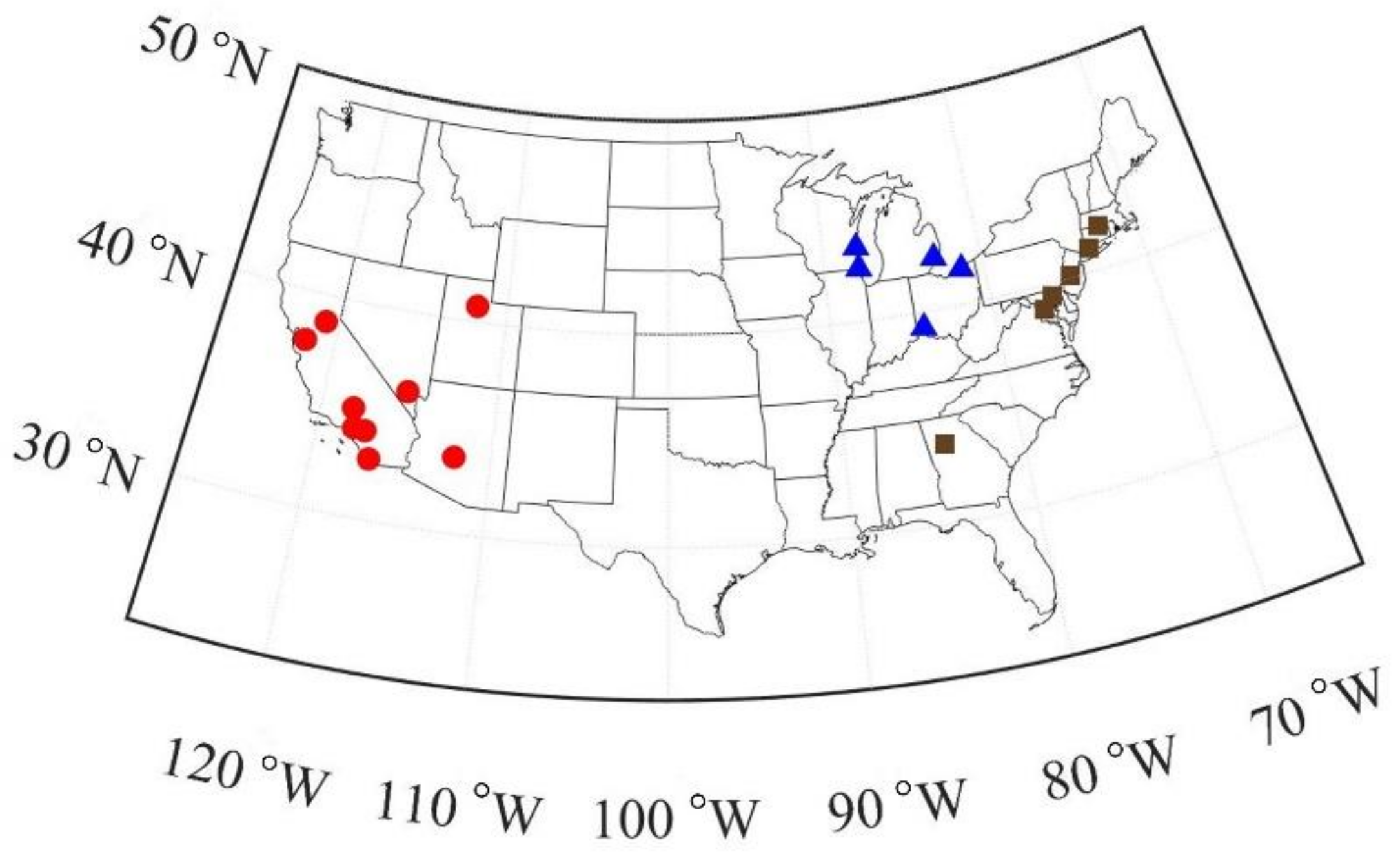
The urban NAAs were grouped into three different regions, which were the eastern, midwestern, and western U.S. (Figure 1 and Table S1). Of the 20 urban NAAs, 6 were in the eastern U.S., 5 were in the midwestern U.S., and 9 were in the western U.S. To assess the relationship between O3 and temperature for time periods when anthropogenic NOx and VOC emissions decreased and surface temperatures increased, the data were separated into three time intervals (1995–2003, 2004–2012, and 2013–2020).
The annual (May–September) slope of the MDA8 O3 versus TMAX relationship (mO3-T) was determined for each site using robust linear regression with bisquare weights in Matrix Laboratory (MATLAB) version R2020a. An example fit is shown in Figure S1. For this regression type, extreme outliers in the data were neglected and mild outliers in the data were downweighted through the use of a tuning constant [30]. We also compared mO3-T values calculated using reduced major axis regression and found very little difference in the results (comparisons not shown).
3. Results and Discussion
Changes in the 5th, 25th, 50th, 75th, and 95th percentile values of MDA8 O3 and TMAX for the urban NAAs in the eastern, midwestern, and western U.S. from 1995–2003 to 2013–2020 are shown in Figure 2. In all regions, the largest decreases in MDA8 O3 occurred at the highest percentiles, consistent with previous studies that examined O3 trends across the distribution of concentrations [5,6,13,31]. The 95th percentile MDA8 O3 concentrations from 1995–2003 to 2013–2020 decreased by 25 ppb (27%) in the eastern U.S., 19 ppb (22%) in the midwestern U.S., and 14 ppb (14%) in the western U.S. These reductions in high-percentile MDA8 O3 indicate that anthropogenic NOx and VOC emission reductions have been highly successful at lowering peak O3 concentrations in these NAAs. Meanwhile, the slight increases in the 5th percentile MDA8 O3 concentrations in each region were likely attributable in part to less titration by NO and/or increases in background O3 levels [5,7,32]. The temperature distributions indicate that TMAX increased from 1995–2003 to 2013–2020 in all regions. Median TMAX increased by 1.1 °C in the eastern U.S., 0.6 °C in the midwestern U.S., and 1.1 °C in the western U.S. This is approximately twice the global temperature increase, which likely reflects an additional influence from urban heat islands [33].
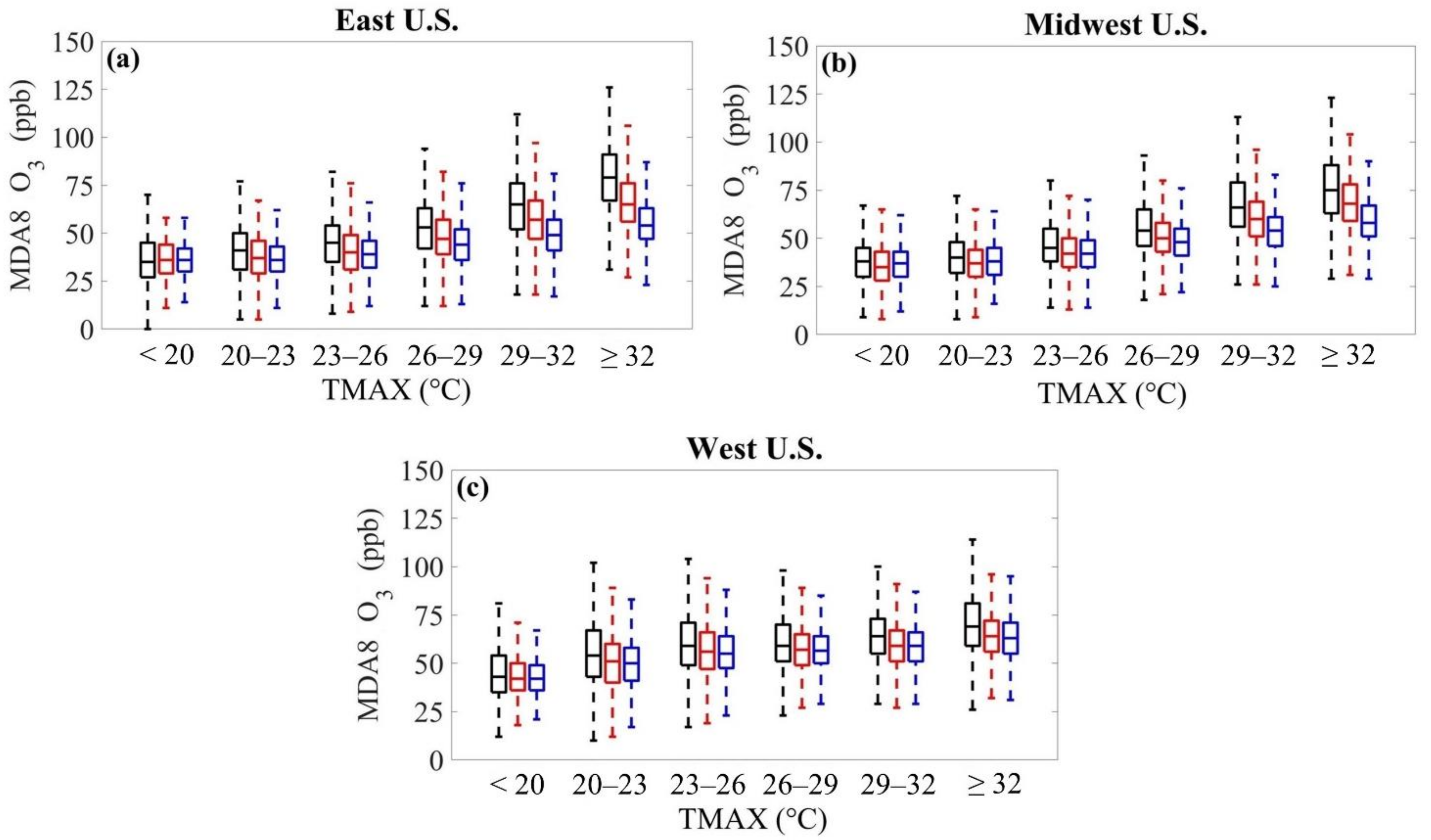
Figure 3 shows the MDA8 O3 concentrations corresponding to six TMAX bins during the 1995–2003, 2004–2012, and 2013–2020 time periods for each region. MDA8 O3 concentrations for the two highest TMAX bins declined in all regions. In the highest TMAX bin, the median MDA8 O3 concentration from 1995–2003 to 2013–2020 decreased from 79 to 54 ppb in the eastern U.S., 75 to 58 ppb in the midwestern U.S., and 69 to 63 ppb in the western U.S. The decreasing MDA8 O3 concentrations at high temperatures show the effectiveness of anthropogenic NOx and VOC emission reductions on lowering peak O3 in the urban NAAs.
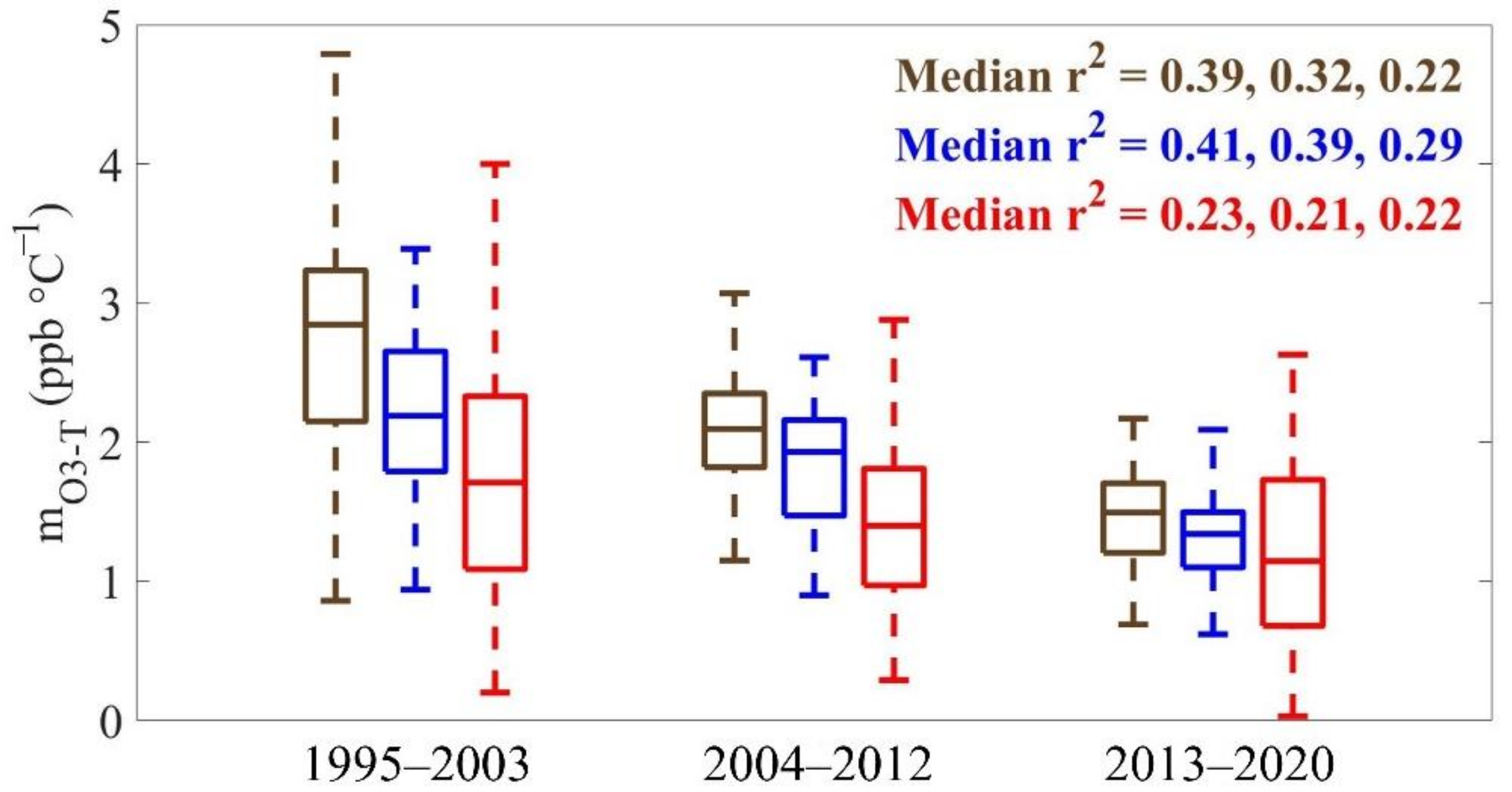
Figure 4 shows the mO3-T values for each region and the median r2 values, grouped into three time periods. Median values of mO3-T from 1995–2003 to 2013–2020 decreased from 2.8 to 1.5 ppb °C−1 in the eastern U.S., 2.2 to 1.3 ppb °C−1 in the midwestern U.S., and 1.7 to 1.1 ppb °C−1 in the western U.S. While the changes in mO3-T are greatest in the eastern U.S. and smallest in the western U.S., the changes in mO3-T for all three regions are statistically significant (p < 0.01). These reductions in mO3-T further demonstrate the success of anthropogenic NOx and VOC emission controls on decreasing peak O3 concentrations.
The steady declines in (1) MDA8 O3 for the highest TMAX bins (Figure 3) and (2) mO3-T and the median r2 values (Figure 4) in the eastern and midwestern U.S. collectively suggest that O3 in those regions has become less correlated with temperature due to emission controls. In contrast, for the western U.S., the combination of smaller decreases in peak MDA8 O3 values and more modest decreases in mO3-T suggest that it will be more challenging for those urban NAAs to achieve compliance with the O3 NAAQS.
Two factors are most important to explain the slower downward trends in mO3-T and MDA8 O3 and the lower r2 values for the O3 versus temperature relationship in the western U.S. First, the hot and dry conditions prevalent in several of the western U.S. cities considered in this study (e.g., Phoenix, Las Vegas, and Bakersfield) often lead to the planetary boundary layer in those areas reaching depths of 3 km or more [34]. As a result, much of the western U.S.—particularly the southwestern U.S.—is more likely to be affected by entrainment of O3-rich lower stratospheric air and O3 transported from Asia. This phenomenon has been found to contribute approximately 20 to 50 ppb to the MDA8 O3 concentration in the southwestern U.S. [35], and it is a significant contributor to the higher background O3 seen in the western U.S. [36]. Second, there have been 10 years with more than 3.2 million ha burned by wildland fires since 2004, and much of the increase in wildfire activity has occurred in the western U.S. [37]. Wildfires emit large but highly variable amounts of O3 precursors (i.e., VOCs and NOx) [38,39,40]. Previous studies have reported that (1) O3 concentrations are higher during smoke-influenced periods compared with smoke-free periods at similar temperatures, and (2) mO3-T values are higher on smoky days than on non-smoky days [41,42,43]. Furthermore, enhanced O3 concentrations due to smoke have been found to lead to elevated O3 levels in western U.S. urban areas [44,45,46]. Thus, it is likely that O3 produced from fire precursors has contributed to the slower rate of decline in mO3-T and MDA8 O3 for the western U.S. The high variability in daily and annual fire emissions also will reduce the correlation between O3 and temperature.
4. Conclusions
This study assessed the observed relationship between O3 and temperature for six, five, and nine urban nonattainment areas (NAAs) in the eastern, midwestern, and western U.S., respectively, over a 26-year period (1995–2020). The 95th percentile maximum daily 8-h average (MDA8) O3 concentration decreased by 25 ppb (27%) in the eastern U.S., 19 ppb (22%) in the midwestern U.S., and 14 ppb (14%) in the western U.S. The median slope of the O3 versus temperature relationship (mO3-T) decreased from 2.8 to 1.5 ppb °C−1 in the eastern U.S., 2.2 to 1.3 ppb °C−1 in the midwestern U.S., and 1.7 to 1.1 ppb °C−1 in the western U.S. These decreases in high-percentile MDA8 O3 and mO3-T indicate the success of anthropogenic NOx and VOC emission reductions. The steady decreases in MDA8 O3 at high temperatures, mO3-T, and the median r2 values in the eastern and midwestern U.S. show that O3 is less dependent on temperature due to emission reductions. Meanwhile, the more modest declines in MDA8 O3 at high temperatures and mO3-T and the lower median r2 values for the O3 versus temperature relationship in the western U.S. demonstrate the influence of higher background O3 and wildfire smoke and show that meeting the O3 standard in the western U.S. continues to be a major challenge.
Supplementary Materials
The following are available online at https://www.mdpi.com/article/10.3390/atmos12101235/s1, Table S1: Site and Data Information for the Urban Nonattainment Areas Considered in this Study, Figure S1: Maximum Daily 8-h Average Ozone Versus Daily Maximum Temperature for Sacramento, CA in May–September 2009.
Author Contributions
Conceptualization, M.N. and D.J.; methodology, M.N. and D.J.; software, M.N.; formal analysis, M.N.; investigation, M.N.; writing—original draft preparation, M.N.; writing—review and editing, D.J.; visualization, M.N.; supervision, D.J.; funding acquisition, D.J. All authors have read and agreed to the published version of the manuscript.
Funding
This research was funded by the National Oceanic and Atmospheric Administration, grant number NA17OAR431001.
Institutional Review Board Statement
Not applicable.
Informed Consent Statement
Not applicable.
Data Availability Statement
The maximum daily 8-h average ozone (MDA8 O3) data used in this study are publicly available via the U.S. EPA’s Air Data system (https://www.epa.gov/outdoor-air-quality-data, accessed on 26 April 2021). The daily maximum temperature (TMAX) data used in this study are publicly available via the NOAA NCEI Global Historical Climatology Network daily (GHCNd) database (https://www.ncei.noaa.gov/products/land-based-station/global-historical-climatology-network-daily, accessed on 26 April 2021). Both data sources are cited in the References [47,48].
Conflicts of Interest
The authors declare no conflict of interest. The funders had no role in the design of the study; in the collection, analyses, or interpretation of data; in the writing of the manuscript; or in the decision to publish the results.
References
- Ebi, K.L.; McGregor, G. Climate Change, Tropospheric Ozone and Particulate Matter, and Health Impacts. Environ. Health Perspect. 2008, 116, 1449–1455. [Google Scholar] [CrossRef]
- Lippmann, M. Health effects of tropospheric ozone. Environ. Sci. Technol. 1991, 25, 1954–1962. [Google Scholar] [CrossRef]
- Zhang, J.; Wei, Y.; Fang, Z. Ozone Pollution: A Major Health Hazard Worldwide. Front. Immunol. 2019, 10, 2518. [Google Scholar] [CrossRef] [PubMed] [Green Version]
- Hidy, G.M.; Blanchard, C.L. Precursor reductions and ground-level ozone in the continental United States. J. Air Waste Manage. Assoc. 2015, 65, 1261–1282. [Google Scholar] [CrossRef]
- Cooper, O.R.; Gao, R.-S.; Tarasick, D.; Leblanc, T.; Sweeney, C. Long-term ozone trends at rural ozone monitoring sites across the United States, 1990–2010. J. Geophys. Res.: Atmos. 2012, 117, D22307. [Google Scholar] [CrossRef]
- Simon, H.; Reff, A.; Wells, B.; Xing, J.; Frank, N. Ozone Trends Across the United States over a Period of Decreasing NOx and VOC Emissions. Environ. Sci. Technol. 2015, 49, 186–195. [Google Scholar] [CrossRef] [PubMed] [Green Version]
- Strode, S.A.; Rodriguez, J.M.; Logan, J.A.; Cooper, O.R.; Witte, J.C.; Lamsal, L.N.; Damon, M.; Van Aartsen, B.; Steenrod, S.D.; Strahan, S.E. Trends and variability in surface ozone over the United States. J. Geophys. Res.: Atmos. 2015, 120, 9020–9042. [Google Scholar] [CrossRef]
- U.S. Environmental Protection Agency (EPA). National Ambient Air Quality Standards for Ozone, 80 Fed. Reg. 65292. Available online: https://www.epa.gov/ground-level-ozone-pollution/ozone-national-ambient-air-quality-standards-naaqs (accessed on 26 October 2015).
- U.S. Environmental Protection Agency (EPA). Ozone Designation and Classification Information. Available online: https://www.epa.gov/green-book/ozone-designation-and-classification-information (accessed on 10 May 2021).
- Chen, Z.; Li, R.; Chen, D.; Zhuang, Y.; Gao, B.; Yang, L.; Li, M. Understanding the causal influence of major meteorological factors on ground ozone concentrations across China. J. Clean. Prod. 2020, 242, 118498. [Google Scholar] [CrossRef]
- Toh, Y.Y.; Lim, S.F.; von Glasow, R. The influence of meteorological factors and biomass burning on surface ozone concentrations at Tanah Rata, Malaysia. Atmos. Environ. 2013, 70, 435–446. [Google Scholar] [CrossRef]
- Zhao, K.; Bao, Y.; Huang, J.; Wu, Y.; Moshary, F.; Arend, M.; Wang, Y.; Lee, X. A high-resolution modeling study of a heat wave-driven ozone exceedance event in New York City and surrounding regions. Atmos. Environ. 2019, 199, 368–379. [Google Scholar] [CrossRef]
- Bloomer, B.J.; Stehr, J.W.; Piety, C.A.; Salawitch, R.J.; Dickerson, R.R. Observed relationships of ozone air pollution with temperature and emissions. Geophys. Res. Lett. 2009, 36, L09803. [Google Scholar] [CrossRef] [Green Version]
- Wu, S.; Mickley, L.J.; Leibensperger, E.M.; Jacob, D.J.; Rind, D.; Streets, D.G. Effects of 2000–2050 global change on ozone air quality in the United States. J. Geophys. Res.: Atmos. 2008, 113, D06302. [Google Scholar] [CrossRef] [Green Version]
- Avise, J.; Abraham, R.G.; Chung, S.H.; Chen, J.; Lamb, B.; Salathé, E.P.; Zhang, Y.; Nolte, C.G.; Loughlin, D.H.; Guenther, A.; Wiedinmyer, C.; Duhl, T. Evaluating the effects of climate change on summertime ozone using a relative response factor approach for policymakers. J. Air Waste Manage. Assoc. 2012, 62, 1061–1074. [Google Scholar] [CrossRef] [PubMed] [Green Version]
- Brown-Steiner, B.; Hess, P.G.; Lin, M.Y. On the capabilities and limitations of GCCM simulations of summertime regional air quality: A diagnostic analysis of ozone and temperature simulations in the US using CESM CAM-Chem. Atmos. Environ. 2015, 101, 134–148. [Google Scholar] [CrossRef] [Green Version]
- Camalier, L.; Cox, W.; Dolwick, P. The effects of meteorology on ozone in urban areas and their use in assessing ozone trends. Atmos. Environ. 2007, 41, 7127–7137. [Google Scholar] [CrossRef]
- Dawson, J.P.; Adams, P.J.; Pandis, S.N. Sensitivity of ozone to summertime climate in the eastern USA: A modeling case study. Atmos. Environ. 2007, 41, 1494–1511. [Google Scholar] [CrossRef]
- Fu, T.-M.; Zheng, Y.; Paulot, F.; Mao, J.; Yantosca, R.M. Positive but variable sensitivity of August surface ozone to large-scale warming in the southeast United States. Nat. Clim. Chang. 2015, 5, 454–458. [Google Scholar] [CrossRef]
- Ito, A.; Sillman, S.; Penner, J.E. Global chemical transport model study of ozone response to changes in chemical kinetics and biogenic volatile organic compounds emissions due to increasing temperatures: Sensitivities to isoprene nitrate chemistry and grid resolution. J. Geophys. Res. Atmos. 2009, 114, D09301. [Google Scholar] [CrossRef]
- Jaffe, D.A.; Zhang, L. Meteorological anomalies lead to elevated O3 in the western U.S. in June 2015. Geophys. Res. Lett. 2017, 44, 1990–1997. [Google Scholar] [CrossRef]
- Olszyna, K.J.; Luria, M.; Meagher, J.F. The correlation of temperature and rural ozone levels in southeastern U.S.A. Atmos. Environ. 1997, 31, 3011–3022. [Google Scholar] [CrossRef]
- Rasmussen, D.J.; Fiore, A.M.; Naik, V.; Horowitz, L.W.; McGinnis, S.J.; Schultz, M.G. Surface ozone-temperature relationships in the eastern U.S.: A monthly climatology for evaluating chemistry-climate models. Atmos. Environ. 2012, 47, 142–153. [Google Scholar] [CrossRef]
- Sillman, S.; Samson, P.J. Impact of temperature on oxidant photochemistry in urban, polluted rural and remote environments. J. Geophys. Res. Atmos. 1995, 100, 11497–11508. [Google Scholar] [CrossRef]
- Steiner, A.L.; Davis, A.J.; Sillman, S.; Owen, R.C.; Michalak, A.M.; Fiore, A.M. Observed suppression of ozone formation at extremely high temperatures due to chemical and biophysical feedbacks. Proc. Natl. Acad. Sci. USA 2010, 107, 19685–19690. [Google Scholar] [CrossRef] [PubMed] [Green Version]
- Pusede, S.E.; Steiner, A.L.; Cohen, R.C. Temperature and Recent Trends in the Chemistry of Continental Surface Ozone. Chem. Rev. 2015, 115, 3898–3918. [Google Scholar] [CrossRef] [PubMed]
- Jin, X.; Fiore, A.M.; Murray, L.T.; Valin, L.C.; Lamsal, L.N.; Duncan, B.; Boersma, K.F.; De Smedt, I.; Abad, G.G.; Chance, K.; Tonnesen, G.S. Evaluating a Space-Based Indicator of Surface Ozone-NOx-VOC Sensitivity Over Midlatitude Source Regions and Application to Decadal Trends. J. Geophys. Res. Atmos. 2017, 122, 10439–10461. [Google Scholar] [CrossRef] [PubMed]
- Jin, X.; Fiore, A.; Boersma, K.F.; De Smedt, I.; Valin, L. Inferring Changes in Summertime Surface Ozone-NOx-VOC Chemistry over U.S. Urban Areas from Two Decades of Satellite and Ground-Based Observations. Environ. Sci. Technol. 2020, 54, 6518–6529. [Google Scholar] [CrossRef]
- Lenssen, N.J.L.; Schmidt, G.A.; Hansen, J.E.; Menne, M.J.; Persin, A.; Ruedy, R.; Zyss, D. Improvements in the GISTEMP Uncertainty Model. J. Geophys. Res. Atmos. 2019, 124, 6307–6326. [Google Scholar] [CrossRef]
- Robustfit: Robust Regression. Available online: https://www.mathworks.com/help/stats/robustfit.html (accessed on 12 May 2021).
- Rieder, H.E.; Fiore, A.M.; Horowitz, L.W.; Naik, V. Projecting policy-relevant metrics for high summertime ozone pollution events over the eastern United States due to climate and emission changes during the 21st century. J. Geophys. Res.: Atmos. 2015, 120, 784–800. [Google Scholar] [CrossRef] [Green Version]
- Lin, C.-Y.C.; Jacob, D.J.; Munger, J.M.; Fiore, A.M. Increasing background ozone in surface air over the United States. Geophys. Res. Lett. 2000, 27, 3465–3468. [Google Scholar]
- Parker, D.E. Urban heat island effects on estimates of observed climate change. WIREs Clim. Chang. 2009, 1, 123–133. [Google Scholar] [CrossRef]
- McGrath-Spangler, E.L.; Denning, A.S. Estimates of North American summertime planetary boundary layer depths derived from space-borne lidar. J. Geophys. Res. Atmos. 2012, 117, D15101. [Google Scholar] [CrossRef] [Green Version]
- Langford, A.O.; Alvarez II, R.J.; Brioude, J.; Fine, R.; Gustin, M.S.; Lin, M.Y.; Marchbanks, R.D.; Pierce, R.B.; Sandberg, S.P.; Senff, C.J.; Weickmann, A.M.; Williams, E.J. Entrainment of stratospheric air and Asian pollution by the convective boundary layer in the southwestern U.S. J. Geophys. Res. Atmos. 2017, 122, 1312–1337. [Google Scholar] [CrossRef]
- Jaffe, D.A.; Fiore, A.M.; Keating, T.J. Importance of Background Ozone for Air Quality Management. The Magazine for Environmental Managers. November 2020, pp. 1–5. Available online: https://pubs.awma.org/flip/EM-Nov-2020/jaffe.pdf (accessed on 24 August 2021).
- National Interagency Fire Center. Fire Information: Statistics. Available online: https://www.nifc.gov/fire-information/statistics (accessed on 11 August 2021).
- Akagi, S.K.; Yokelson, R.J.; Wiedinmyer, C.; Alvarado, M.J.; Reid, J.S.; Karl, T.; Crounse, J.D.; Wennberg, P.O. Emission factors for open and domestic biomass burning for use in atmospheric models. Atmos. Chem. Phys. 2011, 11, 4039–4072. [Google Scholar] [CrossRef] [Green Version]
- Andreae, M.O. Emission of trace gases and aerosols from biomass burning–an updated assessment. Atmos. Chem. Phys. 2019, 19, 8523–8546. [Google Scholar] [CrossRef] [Green Version]
- Lindaas, J.; Pollack, I.B.; Garofalo, L.A.; Pothier, M.A.; Farmer, D.K.; Kreidenweis, S.M.; Campos, T.L.; Flocke, F.; Weinheimer, A.J.; Montzka, D.D.; et al. Emissions of Reactive Nitrogen From Western U.S. Wildfires During Summer 2018. J. Geophys. Res. Atmos. 2020, 125, e2020JD032657. [Google Scholar]
- Flynn, M.T.; Mattson, E.J.; Jaffe, D.A.; Gratz, L.E. Spatial patterns in summertime surface ozone in the Southern Front Range of the U.S. Rocky Mountains. Elementa Sci. Anthr. 2021, 9, 1. [Google Scholar]
- Jaffe, D.A. Evaluation of Ozone Patterns and Trends in 8 Major Metropolitan Areas in the U.S.; A-124; Coordinating Research Council, Inc.: Alpharetta, GA, USA, 2021; Available online: http://crcao.org/wp-content/uploads/2021/04/CRC-Project-A-124-Final-Report_Mar2021.pdf (accessed on 24 August 2021).
- Lindaas, J.; Farmer, D.K.; Pollack, I.B.; Abeleira, A.; Flocke, F.; Roscioli, R.; Herndon, S.; Fischer, E.V. Changes in ozone and precursors during two aged wildfire smoke events in the Colorado Front Range in summer 2015. Atmos. Chem. Phys. 2017, 17, 10691–10707. [Google Scholar] [CrossRef] [Green Version]
- Gong, X.; Kaulfus, A.; Nair, U.; Jaffe, D.A. Quantifying O3 Impacts in Urban Areas Due to Wildfires Using a Generalized Additive Model. Environ. Sci. Technol. 2017, 51, 13216–13223. [Google Scholar] [CrossRef]
- Jaffe, D.A.; Wigder, N.; Downey, N.; Pfister, G.; Boynard, A.; Reid, S.B. Impact of Wildfires on Ozone Exceptional Events in the Western U.S. Environ. Sci. Technol. 2013, 47, 11065–11072. [Google Scholar] [CrossRef]
- McClure, C.D.; Jaffe, D.A. Investigation of high ozone events due to wildfire smoke in an urban area. Atmos. Environ. 2018, 194, 146–157. [Google Scholar] [CrossRef]
- U.S. Environmental Protection Agency (EPA). Air Data: Air Quality Data Collected at Outdoor Monitors Across the US. Available online: https://www.epa.gov/outdoor-air-quality-data (accessed on 26 April 2021).
- National Centers for Environmental Information. Global Historical Climatology Network Daily. Available online: https://www.ncei.noaa.gov/products/land-based-station/global-historical-climatology-network-daily (accessed on 26 April 2021).
Figure 1.
Map showing the locations of the O3 monitoring sites for the urban nonattainment areas (NAAs) in the eastern U.S. (brown squares), midwestern U.S. (blue triangles), and western U.S. (red circles). See Table S1 for a list of the urban NAAs for the eastern, midwestern, and western U.S.
Figure 1.
Map showing the locations of the O3 monitoring sites for the urban nonattainment areas (NAAs) in the eastern U.S. (brown squares), midwestern U.S. (blue triangles), and western U.S. (red circles). See Table S1 for a list of the urban NAAs for the eastern, midwestern, and western U.S.

Figure 2.
Maximum daily 8-h average (MDA8) O3 (ppb; panels (a–c)) and daily maximum temperature (TMAX, °C; panels (d–f)) during the O3 season (May–September) for urban nonattainment areas (NAAs) in the eastern U.S. (left column), midwestern U.S. (middle column), and western U.S. (right column). The x-axes indicate the 5th percentile (black), 25th percentile (green), 50th percentile (dark blue), 75th percentile (gold), and 95th percentile (light blue) of the May–September 1995–2003 data. The y-axes indicate how much the 5th, 25th, 50th, 75th, and 95th percentiles of the MDA8 O3 or TMAX changed from May–September 1995–2003 to May–September 2013–2020.

Figure 3.
Maximum daily 8-h average (MDA8) O3 (ppb) versus daily maximum temperature (TMAX; °C) for six temperature bins for urban nonattainment areas (NAAs) in (a) the eastern U.S., (b) the midwestern U.S., and (c) the western U.S. This relationship was examined across three time intervals: 1995–2003 (black), 2004–2012 (red), and 2013–2020 (blue). All boxplots were generated using coincident MDA8 O3 and TMAX data collected from May to September. The top and bottom whiskers denote the maximum and minimum MDA8 O3 concentrations, respectively, that are not considered outliers, the central rectangles span the 25th percentile to the 75th percentile, and the horizontal lines within the central rectangles represent the median MDA8 O3 concentrations.

Figure 4.
The slope of the maximum daily 8-h average O3 versus the daily maximum temperature (mO3-T; ppb °C−1) for the urban nonattainment areas (NAAs) in the eastern U.S. (brown), midwestern U.S. (blue), and western U.S. (red) from 1995–2003, 2004–2012, and 2013–2020. All slopes were found using coincident MDA8 O3 and TMAX data collected from May to September. The components of each boxplot have the same meanings as in Figure 3. Median r2 values of the O3 versus temperature relationship for each region are listed for the 1995–2003 (first values), 2004–2012 (second values), and 2013–2020 (third values) time periods.

Publisher’s Note: MDPI stays neutral with regard to jurisdictional claims in published maps and institutional affiliations. |
© 2021 by the authors. Licensee MDPI, Basel, Switzerland. This article is an open access article distributed under the terms and conditions of the Creative Commons Attribution (CC BY) license (https://creativecommons.org/licenses/by/4.0/).
Share and Cite
MDPI and ACS Style
Ninneman, M.; Jaffe, D. Observed Relationship between Ozone and Temperature for Urban Nonattainment Areas in the United States. Atmosphere 2021, 12, 1235. https://doi.org/10.3390/atmos12101235
AMA Style
Ninneman M, Jaffe D. Observed Relationship between Ozone and Temperature for Urban Nonattainment Areas in the United States. Atmosphere. 2021; 12(10):1235. https://doi.org/10.3390/atmos12101235
Chicago/Turabian StyleNinneman, Matthew, and Daniel Jaffe. 2021. "Observed Relationship between Ozone and Temperature for Urban Nonattainment Areas in the United States" Atmosphere 12, no. 10: 1235. https://doi.org/10.3390/atmos12101235
Note that from the first issue of 2016, this journal uses article numbers instead of page numbers. See further details here.