Article

Sensitivity of Simulations of Extreme Mediterranean Storms to the Specification of Sea Surface Temperature: Comparison of Cases of a Tropical-Like Cyclone and Explosive Cyclogenesis

Department of Geography and Environment, Bar Ilan University, Ramat Gan 5290002, Israel
*
Author to whom correspondence should be addressed.
Atmosphere 2021, 12(7), 921; https://doi.org/10.3390/atmos12070921
Submission received: 28 May 2021 / Revised: 14 July 2021 / Accepted: 15 July 2021 / Published: 17 July 2021
(This article belongs to the Section Meteorology)

Abstract

:
Local air-sea interaction over the Mediterranean may amplify the effects of climate change. This study investigates the sensitivity of simulations of two different high impact weather events to changes in the specification of sea surface temperature (SST) using a regional atmospheric model. First we assess the impact of specifying SST from two reanalysis data sets with differing spatial resolution. The simulated tropical-like cyclone (TLC) is slightly stronger in the case of the lower resolution SST which is warmer over the formation region, most notably in the maximum rainfall which is ~7% higher. The differences in the two explosive cyclone simulations are negligible, most likely due to intensification occurring mainly over land. We then test the sensitivity of the storms to a range of SST anomalies. The TLC showed a clear trend of increasing storm intensity as SST rises. These results suggest that SST plays a direct role in determining the intensity of the storm. For the explosive cyclone there is no clear trend in dynamical intensity except for the highest warming anomalies. However, the rainfall increases with the magnitude of the SST anomaly. Our results suggest that extreme weather events over the Mediterranean will become more extreme if SST increases as the climate warms, assuming that upper air conditions do not change.

1. Introduction

Geographically, the Mediterranean region is unique in many ways. It is characterized by a Mediterranean climate type with hot, dry summers and cool wet winters. It is centered on a relatively large and warm body of water surrounded by mountain ranges, bounded by the subtropical deserts to the south and the temperate mid-latitudes to the north. The semi-enclosed Mediterranean Sea is subjected to excess evaporation (E − P > 0) and limited connection to the Atlantic Ocean, both of which drive an inverse estuarine circulation in a sea that is relatively warm and saline compared to the adjacent ocean at the same latitudes. Consequently, significant air-sea interaction plays a major role in shaping both the atmospheric and oceanic circulation in this region over a large range of spatial and temporal scales. While the Mediterranean Sea is small relative to the large ocean basins where the most intense storms are frequently formed, the unique combination of the geographical and climate factors leads to the frequent occurrence of high impact weather events such as intense cyclones, strong winds, heavy precipitation and flooding in the cool season as well as prolonged heat waves in summer and multiyear droughts [1]. Two such processes which are the focus of this paper are (1) Mediterranean hurricanes (medicanes), which are tropical-like cyclones (TLC) and (2) meteorological bombs or bomb cyclones, which are referred to as explosive cyclogenesis. Both fall under the broad category of extreme cyclones.

1.1. Tropical-Like Cyclones (Medicanes)

Some Mediterranean cyclones exhibit features similar to tropical cyclones in their mature stage with sustained winds over 100 km/h, and due to their resemblance to tropical cyclones, they are often referred to as medicanes [2]. They are intense low-pressure systems that exhibit some distinct features of the tropical cyclones, such as a cloud free area at the center with an eye, spiral cloud bands with deep convection, a warm core and intense surface winds [3]. Medicanes may occur throughout the year but are most frequent in fall and winter when the sea surface temperature (SST) is still relatively high (although less than 26 °C) and cold air intrusions occur as a consequence of the weakening of the summer anticyclone over Europe [2]. They are triggered by upper tropospheric precursors, such as baroclinic cut-off lows and troughs, similar to polar lows [4], but in contrast to the polar lows, medicanes develop a warm core and minimal wind shear. In addition, abundant moisture and vorticity enhance the genesis of medicanes. It is estimated that an average of about 1.6 medicanes occur each year [5].
Since SST influences the atmosphere through surface fluxes of latent heat and sensible heat [6], many studies of medicances development have focused on air-sea interactions and on the resulting diabatic heating [4,7]. Some studies suggest that these fluxes can influence the storm track and intensification of medicanes, while others suggest that orography, potential vorticity (PV) or jet streams can influence the formation and evolution of the storm [2]. Tropical-like cyclones tend to develop within environments of relatively high diabatic heating [7], but in a range of SST of 15–23 °C [7,8], which is below the accepted cutoff value of 26 °C for the development of tropical cyclones [9], but similar to conditions under which other intense Mediterranean cyclones develop.

1.2. Explosive Cyclones (Meteorological Bombs)

Explosive cyclogenesis, which leads to the development of so-called meteorological bombs or bomb cyclones, is characterized by exceptionally and unusually large deepening rates, resulting in heavy rain, gale force winds and high significant wave heights [10]. Such storms occur mainly during the cold period of the year. The four most active regions where extratropical explosive cyclogenesis occurs in the world are the Northwest Pacific, the North Atlantic, the Southwest Pacific and the South Atlantic [11], but they also are known to occur over the Mediterranean Sea in winter. The change in pressure needed to classify a case as explosive cyclogenesis is latitude dependent compared to the reference values at 60° latitude according to the formula [12]:
Δp/Δt = 24 (sin Φ/sin 60) hPa/24 h
where p is pressure, t is time and Φ is latitude in degrees. Thus, for the central or eastern Mediterranean region at 35° N latitude, a cyclone with a deepening rate of 15.9 hPa or more in 24 h (sustained deepening rate of more than 0.66 hPa h−1) is classified as a case of explosive cyclogenesis.
Baroclinic instability is one of the principal mechanisms for the development of most explosively deepening cyclones especially for the western and central parts of the Mediterranean basin [13]. Other factors include the relative position of the 500 hPa trough and associated thickness patterns, or the so called KF and CC mechanisms. The KF mechanism is characterized by the interaction between a larger scale wave penetrating the Mediterranean basin from northwest and a small-scale cyclone in the lee of the Alps. The CC mechanism is characterized by the interaction between a mid-latitude depression of African origin with a larger-scale cyclone entering the Mediterranean from the north [13]. According to other studies, the SST’s influence on the atmosphere through the latent and sensible heat fluxes plays an important role [6] and therefore some studies focused on air-sea interaction and on the resulting diabatic heating [4,7]. Kouroutzoglou et al. [13] showed that the eastern part of the Mediterranean Sea is a preferred region for the development of deeper explosive cyclones triggered mainly by orographic effects. They also showed that in the western and central Mediterranean Sea the potential vorticity plays an important role in explosive cyclones with low level cold air penetrations from the north, while to the east the upper-level forcing appears to interact with a warmer low level environment leading to significant diabatic forcing [13].
Even though the upper-level circulation is important for the development of the storm, in most cases the surface low is formed before the 500 hPa trough or low, implying a preference towards surface development, emphasizing the importance of low-level forcing [13]. The fact that the eastern Mediterranean basin is warmer than the central and western Mediterranean [14] could possibly explain why the eastern Mediterranean basin is the preferred region for deeper explosive cyclogenesis and how the SST values could influence the storm tracks and intensification.

1.3. Sensitivity of Storm Development to the Specification of SST

Due to the confined nature of the Mediterranean, intense storms that develop over the sea will very likely affect the adjacent land mass and subsequently pose danger to infrastructure, property and life. The storm tracks and intensification may be sensitive to smaller scale details of SST which may be misrepresented in coarser resolution models and data. An effective approach to assessing importance of these details is to run a series of dynamical downscaling simulations with a regional model that can simulate processes that are unresolved in coarser resolution reanalysis data sets.
Often these storms are difficult to predict with operational models. This limitation depends on many factors ranging from the horizontal grid resolution to the subgrid scale physical parameterization schemes which play an important role in the fidelity of the simulations. Lateral and lower boundary conditions such as the SST field, are important and thus coupled ocean-atmosphere modeling systems may be considered as useful for improving the simulation skill [15], although the main benefit of the coupled model is most likely realized mainly in longer time period simulations. Similarly, Tiesi et al. [16] found that specification of initial conditions, with a focus on the addition of high-resolution satellite derived wind fields, can have a noticeable impact on nowcasts and short-range forecasts of various categories of severe Mediterranean storms, including TLCs.
Ricchi et al. [15] showed that the air-sea interaction processes are fundamental for the proper numerical simulation of the storm, and when substituting the real sea surface temperature with an average field it may dramatically affect the intensity of the storm. They also showed that a coupled model could increase the accuracy of the simulations even for short periods of a few days. Nevertheless, they concluded that the choice and combination of physical parameterization schemes in the model that produce the best simulation for one case may not be the best for other cases [15]. Similar results were obtained by Miglietta et al. [17] and Pytharoulis et al. [18]. In contrast to these approaches [15,16,17,18] where model components were swapped and mixed (mainly subgrid scale parameterization schemes), here our approach is to use a fixed model configuration and to focus on a single factor—the specification of SST.
The Mediterranean region has been identified as a climate change hotspot, which may be especially vulnerable to the influence of global change [19]. The effects of air-sea interaction may be amplified or exaggerated by global warming and the increase of the sea surface temperature may lead to an increase in the intensity of extreme events. Therefore, it is important to study the sensitivity of these high impact weather events to potentials changes in SST. Our goal is to examine the sensitivity of simulations of case studies of a tropical-like cyclone and an explosive cyclone to the specification of sea surface temperature (SST) by using regional atmospheric model forced with high spatial resolution SST data as compared to the lower resolution fields typically included in reanalysis data sets.
This manuscript is structured as follows: Section 2 contains a description of the synoptic settings of the two test cases that are studied here—the medicane that developed in December 2005 over the central Mediterranean and the explosive cyclone that developed over the Aegean Sea in December 2010. In Section 3 we present the regional atmospheric model and experimental design. The results are presented in Section 4 and Section 5 contains the discussion and conclusions.

2. Synoptic Summary of the Two Test Cases

In this study we have chosen to assess the influence of SST on the development and intensification of two extreme cyclones that developed over different regions of the Mediterranean Sea. The first is a tropical-like cyclone (TLC) that developed over the central Mediterranean in December 2005. The second is a case of extreme cyclogenesis that occurred over the Aegean Sea (eastern Mediterranean) in December 2010. These two cases were chosen to be representative of two types of extreme cyclones that are initiated by different meteorological processes and therefore have different characteristics as noted in the introduction. The synoptic summaries presented in this section are based on data extracted from the ERA5 hourly data [20] which has a spatial resolution of 0.25°.

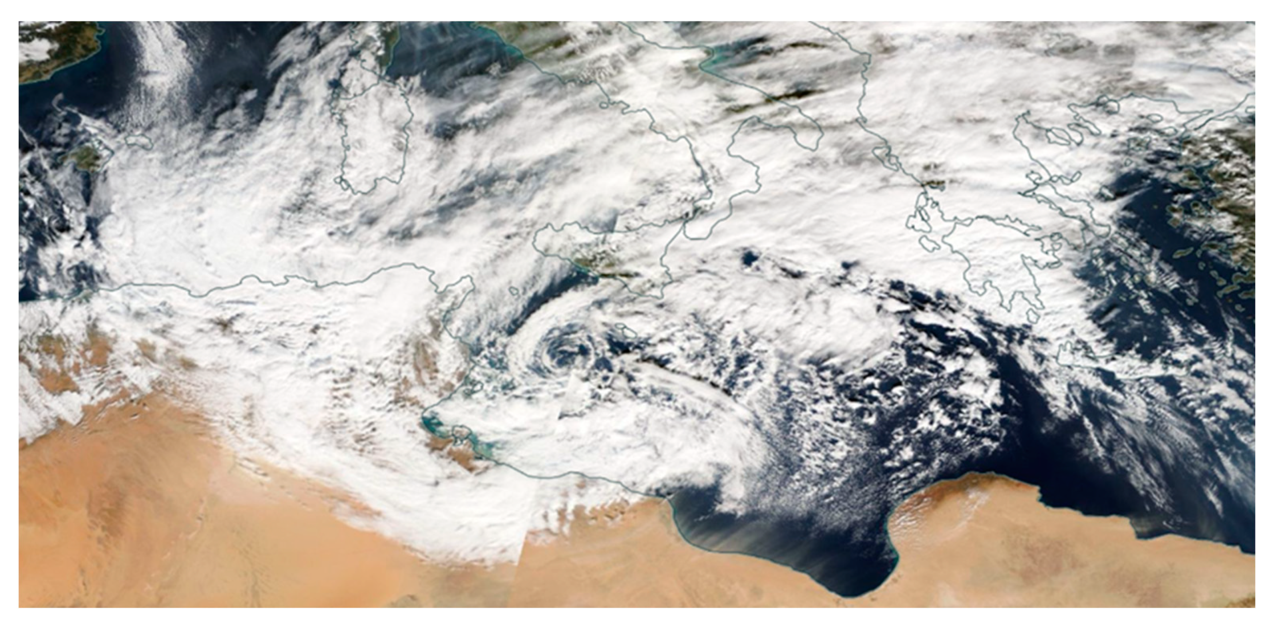
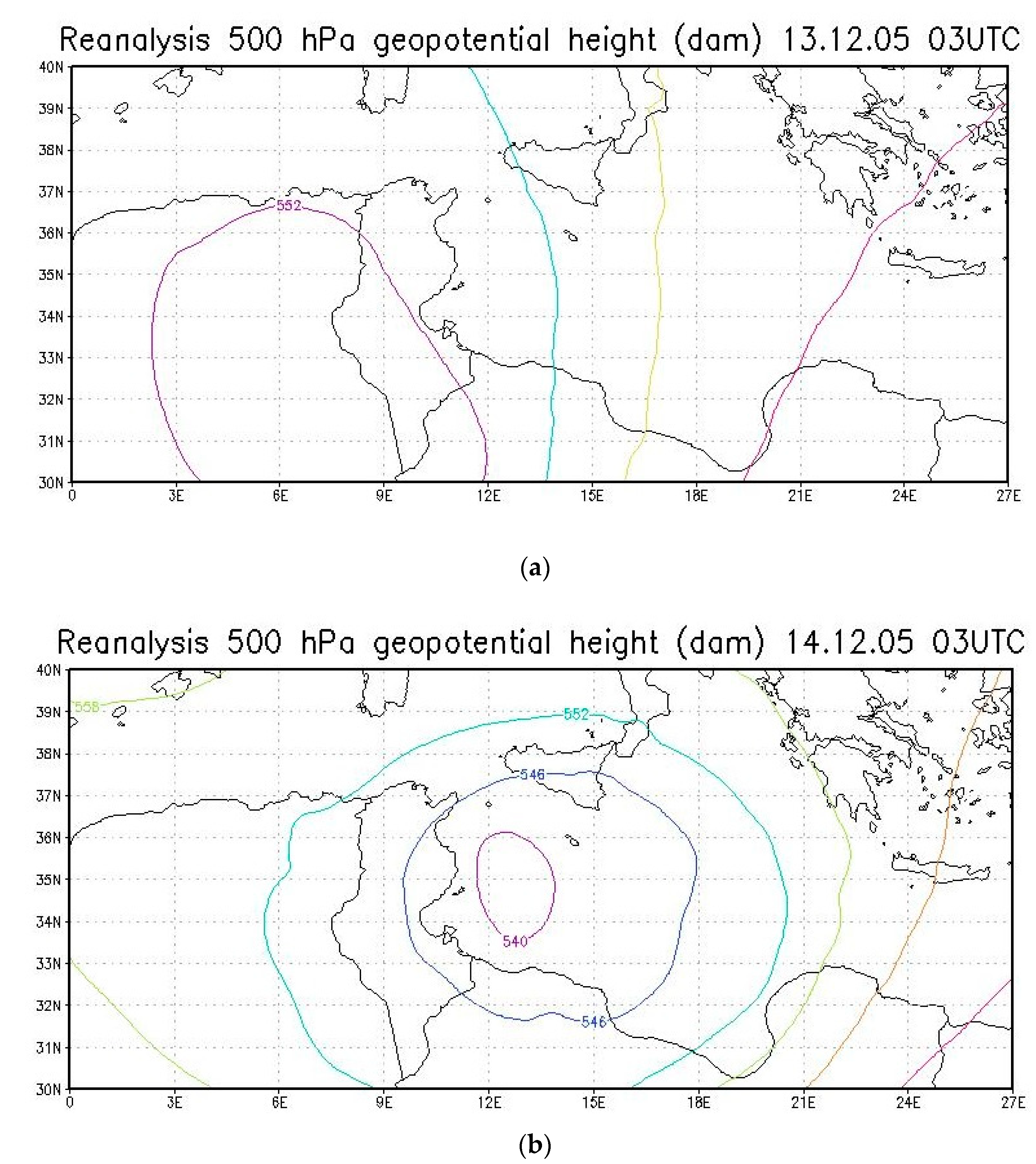
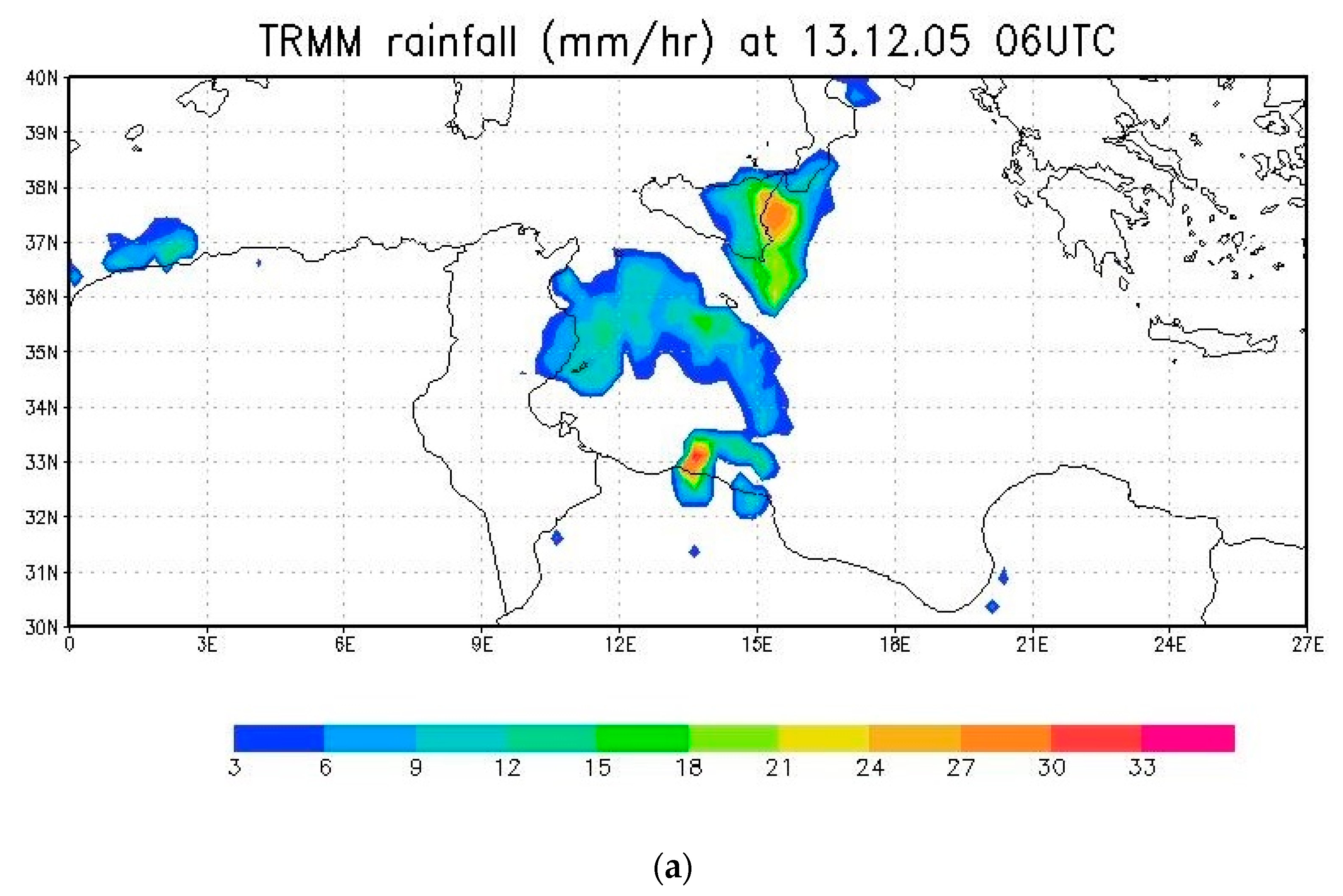
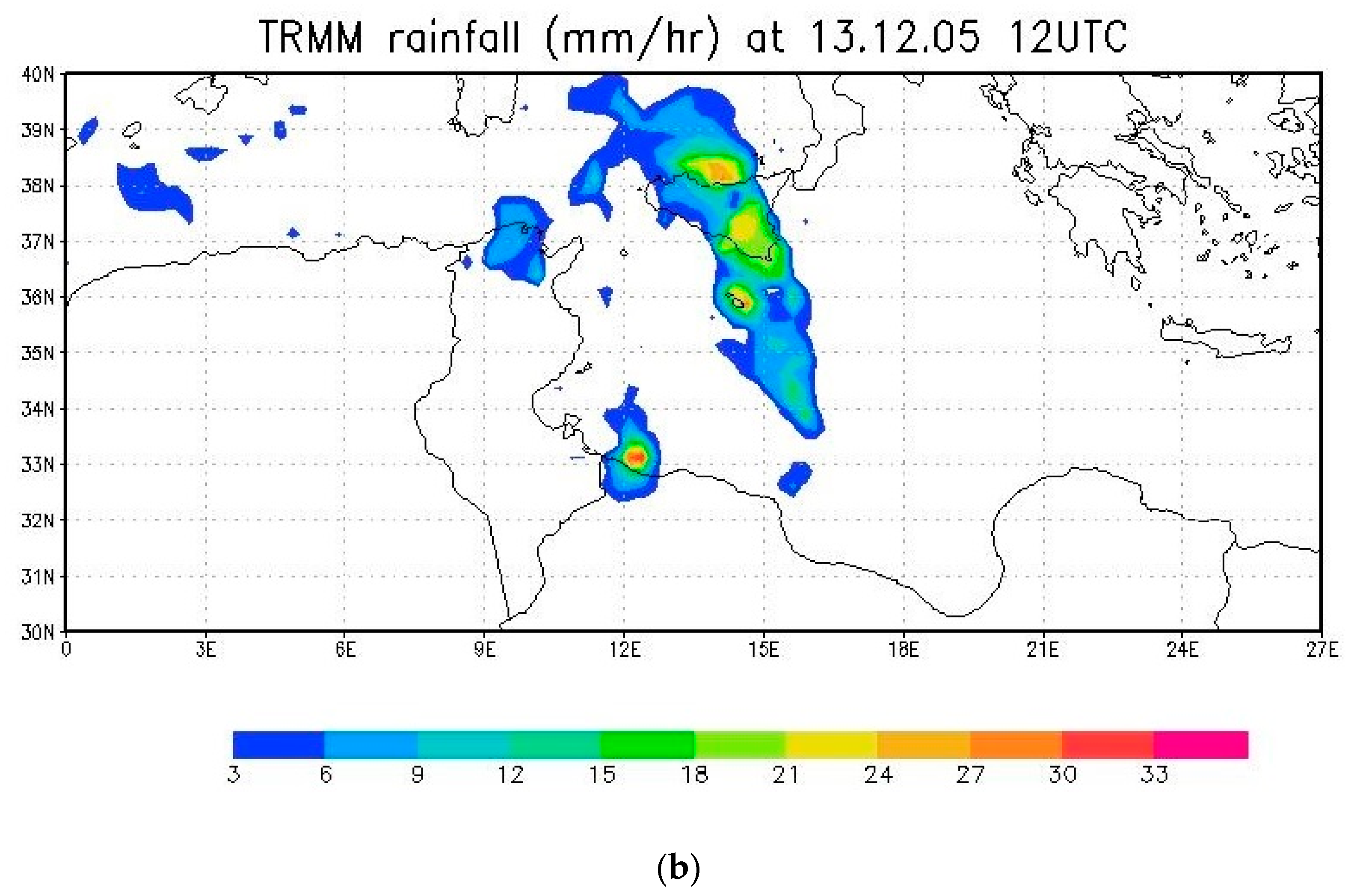
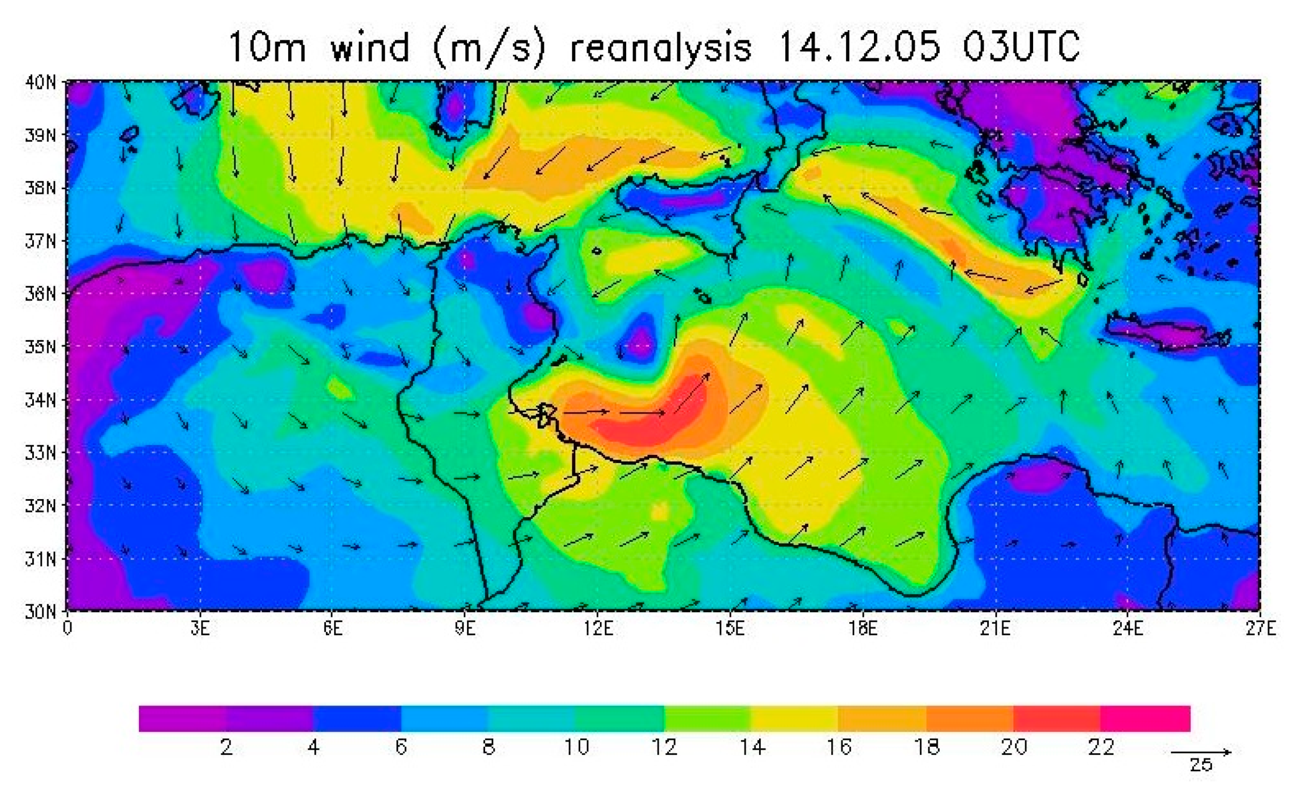
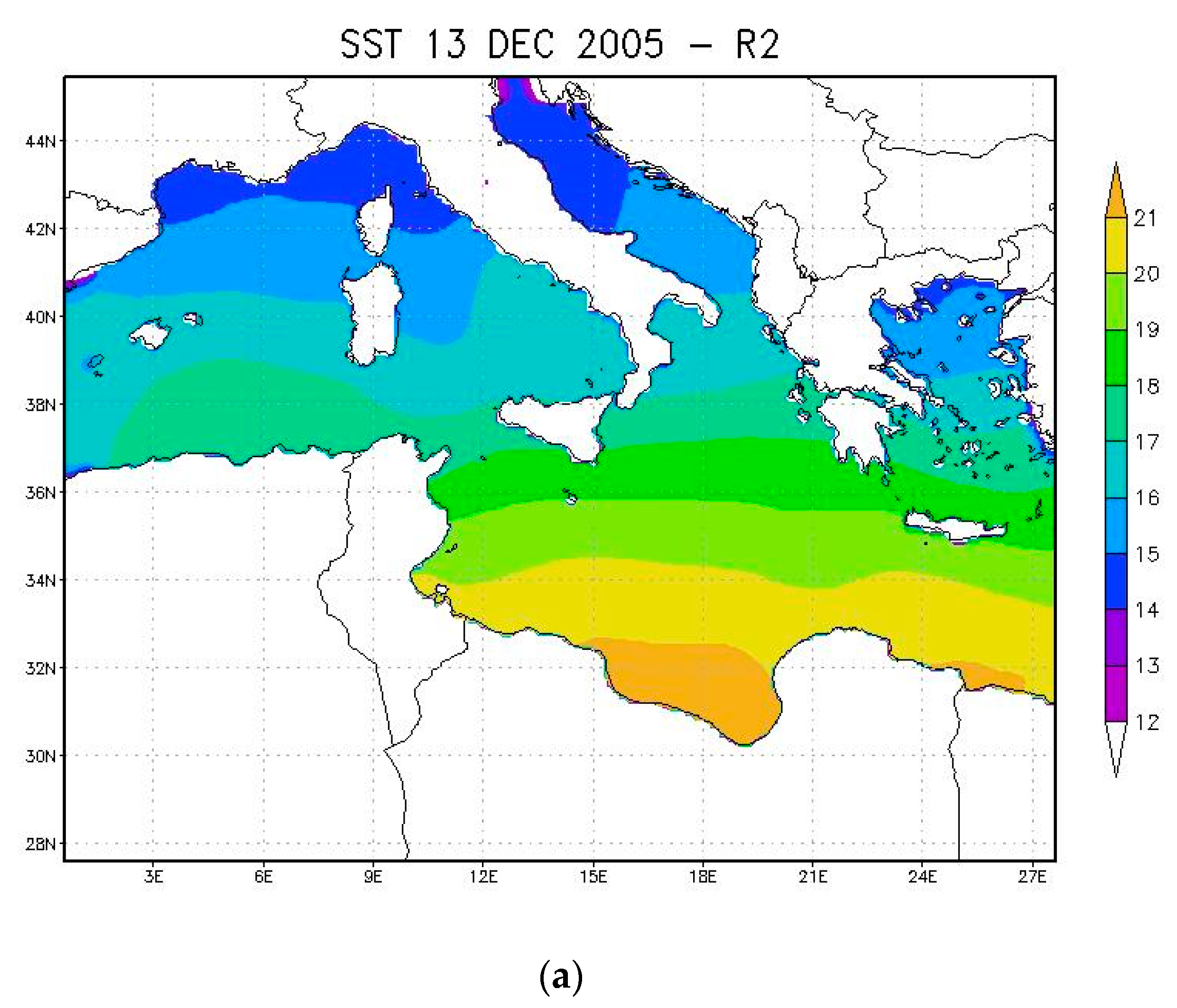
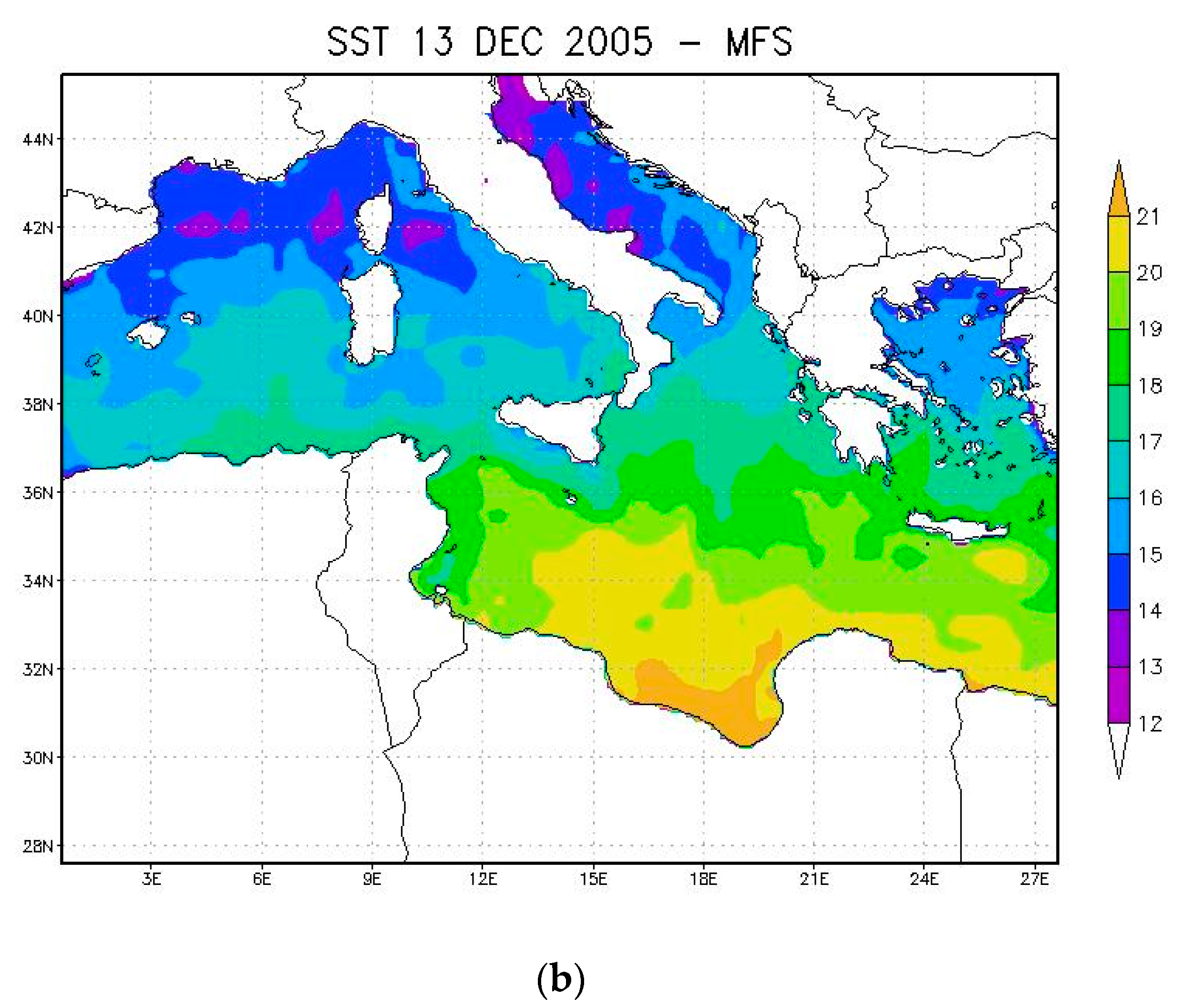
2.1. The Tropical-Like Cyclone of December 2005

This TLC was initially identified on 12 December 2005 18 UTC over Libya as a very weak low-pressure center of about 1009 hPa when the SST was around 18–19 °C [9]. The storm deepened and attained its lowest mean sea level pressure value on 14 December 2005 03 UTC (Figure 1) and remained more or less stationary until 14 December 2005 16:00 UTC. It then moved to the east and crossed nearly the entire Mediterranean basin, while maintaining a low level, asymmetric warm core [9]. The storm decayed on 16 December 2005 over the Levantine basin [21].
At the early stages an upper air, large cutoff low appeared at 500 hPa over northern Algeria with cold air advected from west Europe to the Mediterranean Sea and drier, warm air advected from north Africa, which produced a surface low over northern Libya on 12 December 2005 18:00 UTC with a central mean sea level pressure (MSLP) of 1009 hPa [4]. As the surface low began to deepen, a low-level warm core began to develop due to the warm advection from the south [4]. By 13 December 2005 at 03:00 UTC the cutoff, upper air low was well defined (Figure 2a) and the storm exhibited an axisymmetric structure. As the system moved to the northeast, the 500 hPa low intensified (Figure 2b) as did the surface low. The minimum MSLP of 989.6 hPa was attained at 03:00 UTC on 14 December 2005 (Figure 3). Maximum rainfall occurred during the morning of 13 December 2005 along a north-south cold front extending from Sicily to the coast of Libya (Figure 4) with maximum hourly values of more than 30 mm h−1 over Sicily [22]. By the evening of 13 December 2005, the rainfall around the storm center decayed significantly.
The 10 m wind at the time of the peak of the storm is shown in Figure 5 with maximum sustained wind speeds of 20–22 m s−1 along the southern flank of the low center along the coat of Libya (Figure 5). The strongest winds of 29 m s−1 (104 km h−1) were observed on 13 December 2005 17 UTC before the MSLP reached its lowest value [9]. On 14 December 2005 00 UTC, the TLC fronts clearly showed a T-bone structure following the Shapiro-Keyser cyclone model [9], where the cold front moves perpendicular to the warm front without touching and the gap between the fronts is filled by warmer air masses, thereby leading to the “hammerhead” T-bone structure [23].
A small re-intensification of the upper-level system occurred around mid-day on 14 December 2005, that was followed by rain and convection [21] and a clearly defined eye was observed. At this time the storm remained nearly stationary, located east of Tunis and south of Sicily. Late that day the TLC propagated to the east, maintaining its warm core and the axisymmetric structure until it weakened and decayed over the eastern Levantine basin on the morning of 16 December 2005 [21].

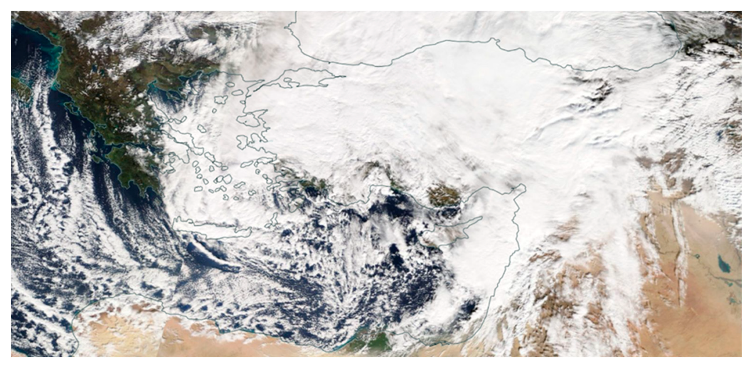
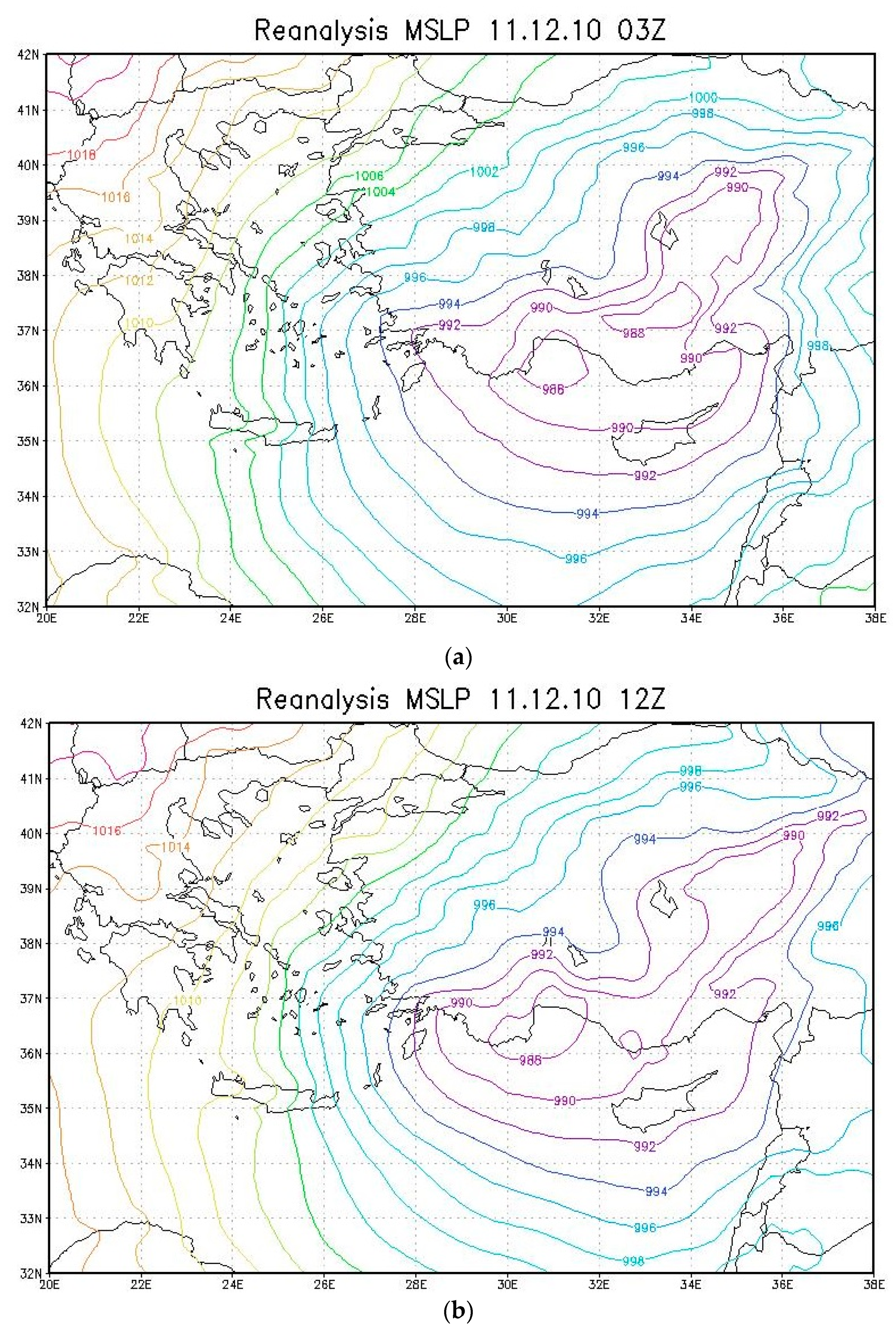
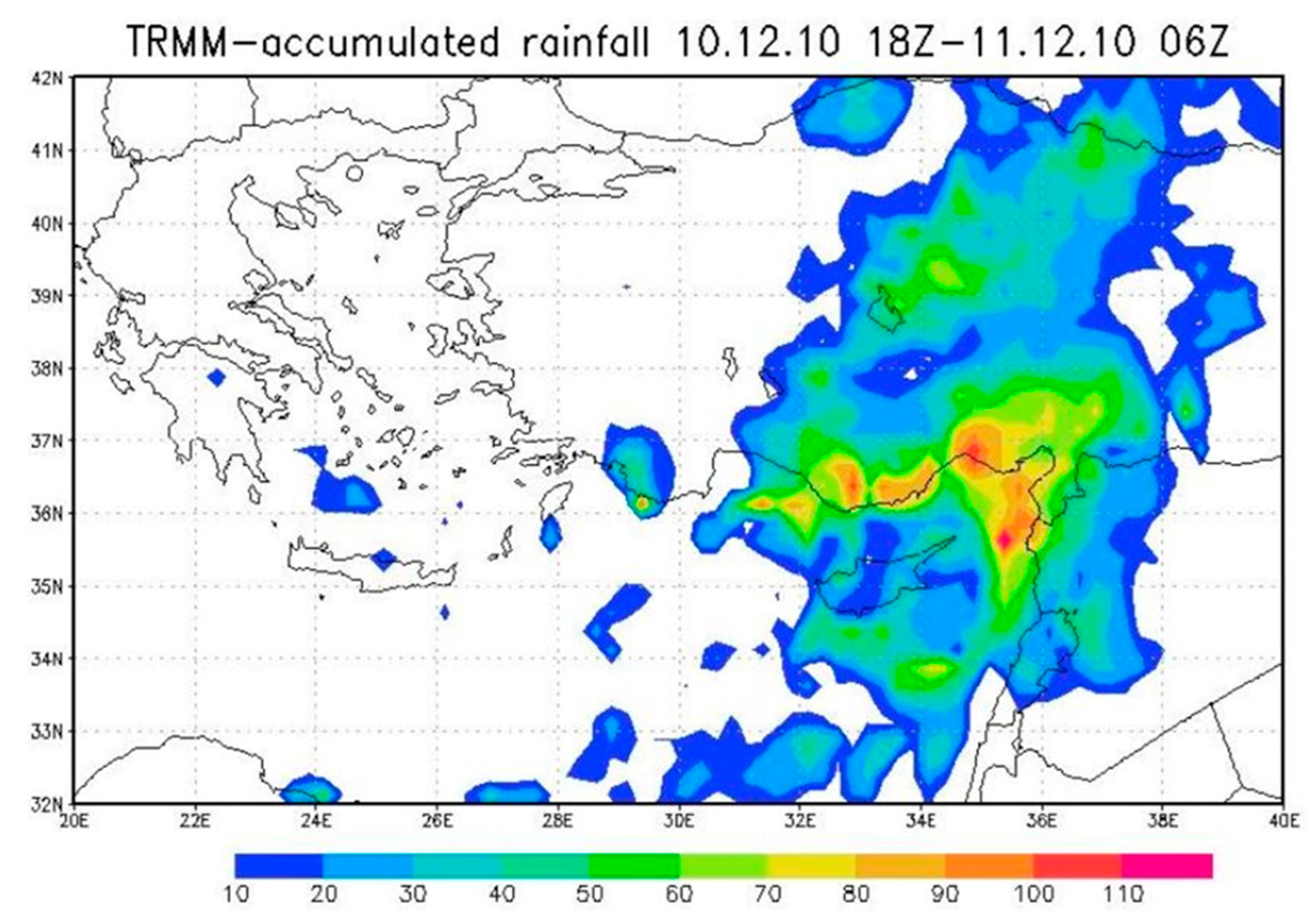
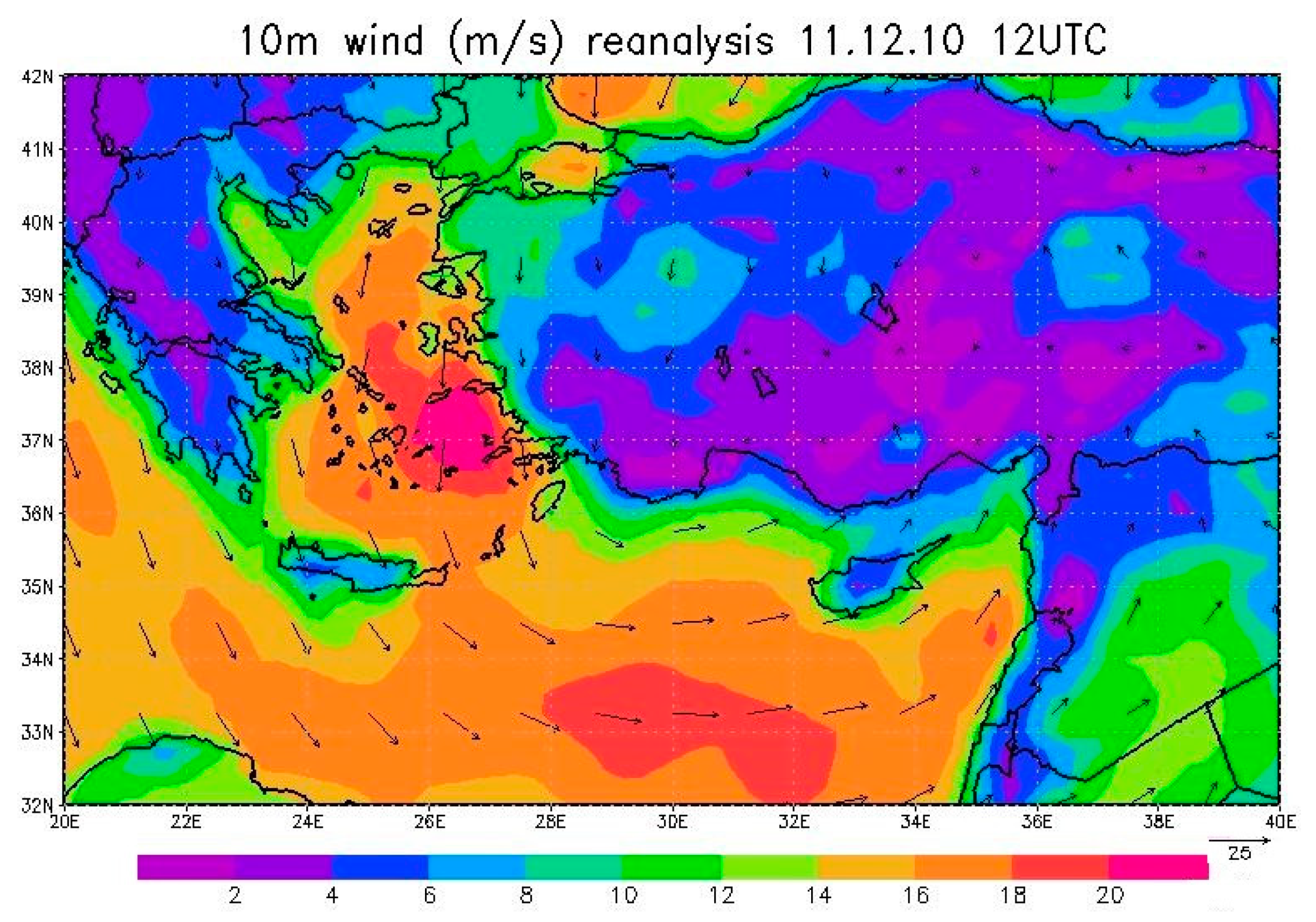
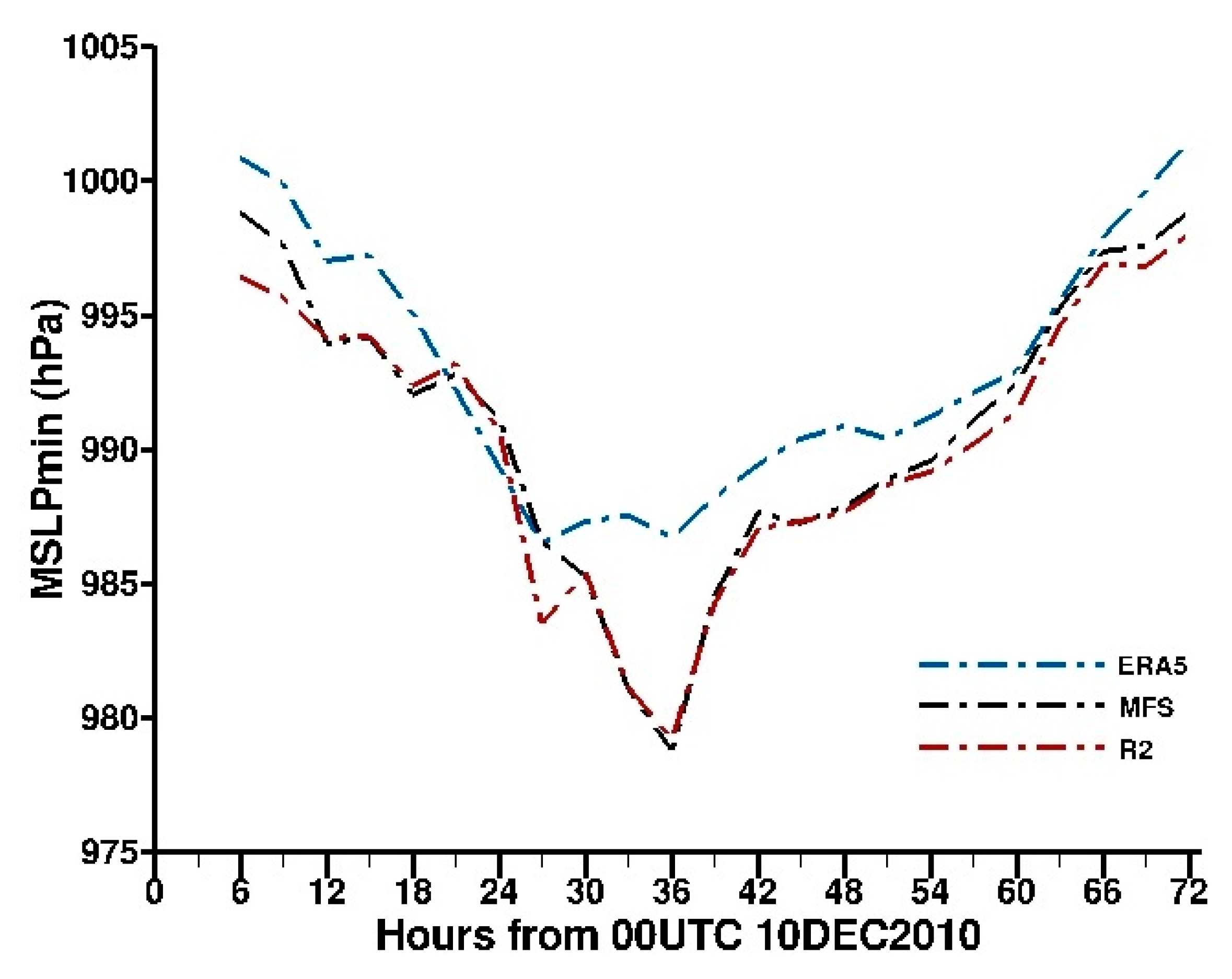
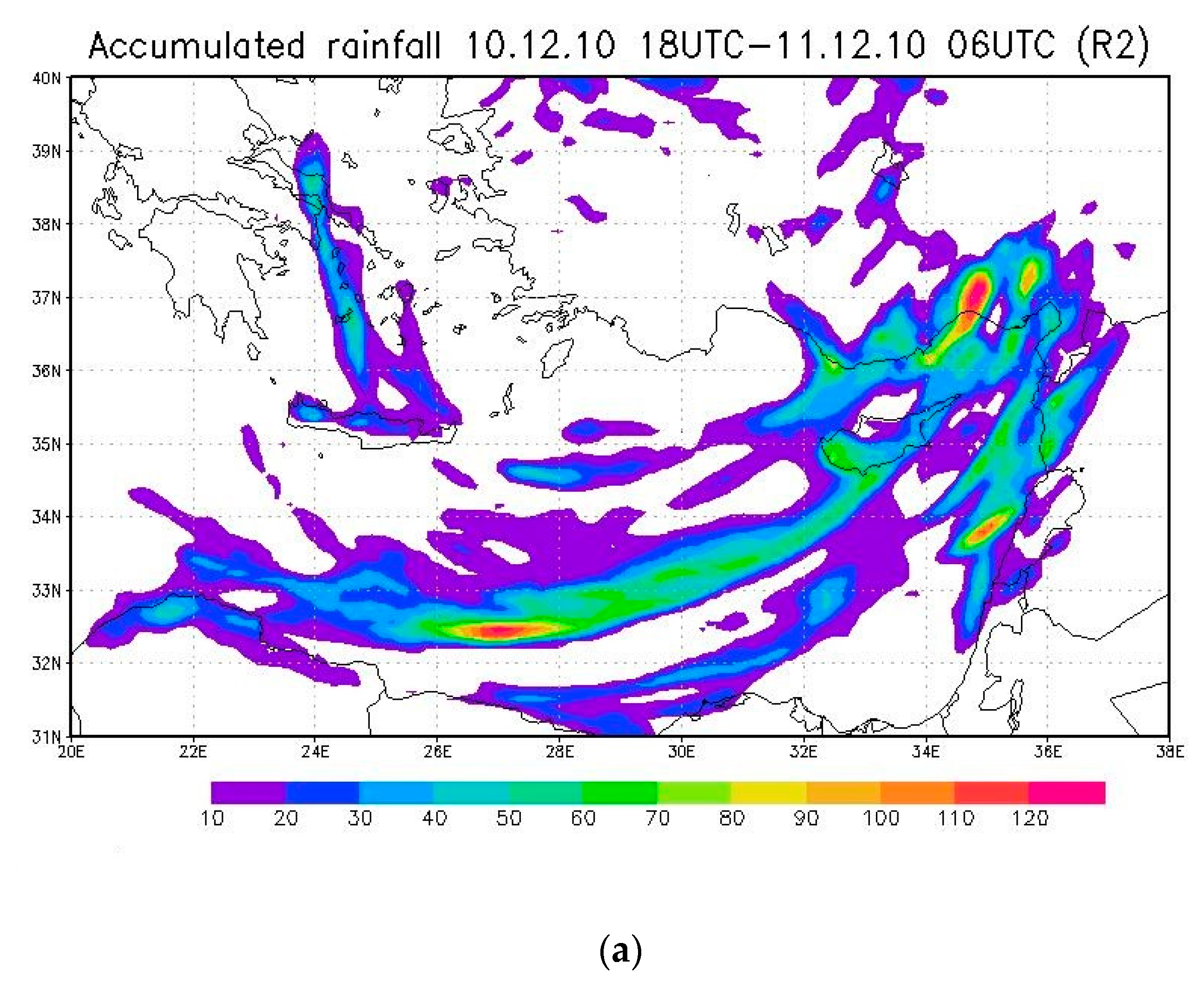
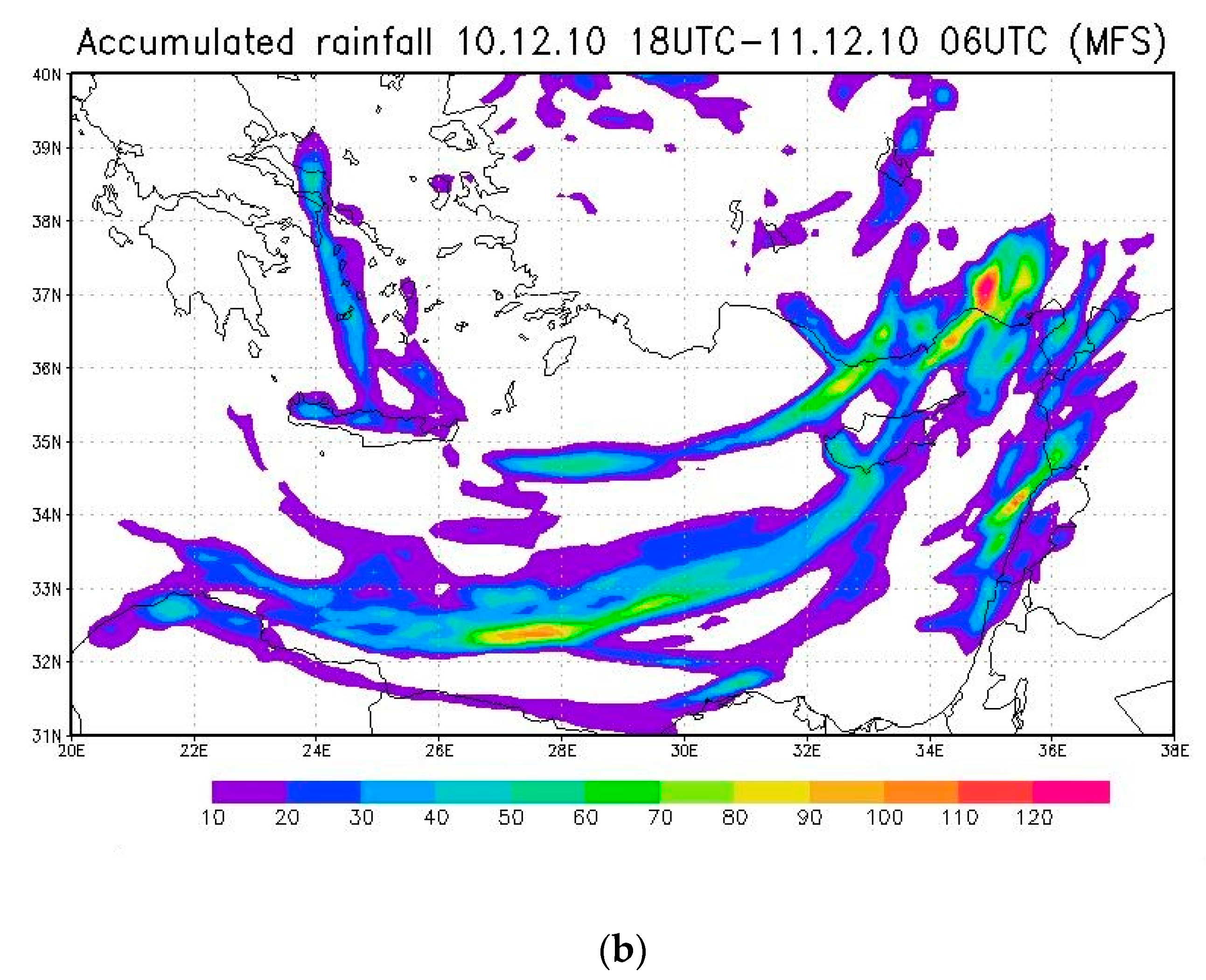
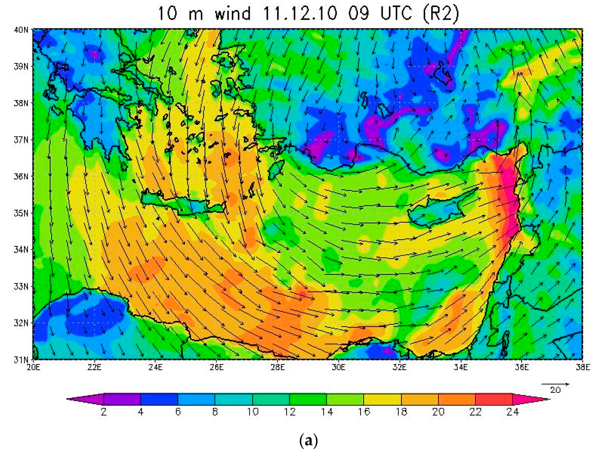
2.2. The Explosive Cyclone of December 2010

In December 2010 an explosive cyclone developed over the eastern Mediterranean. The surface low developed from a trough that extended from the northeast to the Aegean Sea. A closed isobar of 1002 hPa first appeared over the northern Aegean Sea on 10 December 2010 03UTC.The system tracked southeastward into southern Turkey and then eastward along the coast, attaining meteorological bomb status as it intensified over the Gulf of Antalya during 10–11 December 2010 (Figure 6). It then moved to the northeast while a secondary explosive cyclone formed over the same area [13]. The storm caused extremely high waves along the eastern coast of the Mediterranean with maximum significant wave heights of more than 7.5 m recorded off the coast of Haifa, Israel, which were the highest values measured over the past 30 years. SSTs off the coast of Turkey at that time were in the range of 20–22 °C suggesting that cold air advection from the north over the warm sea significantly contributed to the rapid intensification of the storm [10].
The storm became explosive as the sea level pressure dropped rapidly from 995.1 to 986.5 hPa between 10 December 2010 18 UTC and 11 December 2010 03 UTC, initially as it remained over the sea and then as the surface low moved over land to the northeast as shown in Figure 7a. The pressure drop of 8.6 hPa over 9 h was above the cutoff for explosive cyclogenesis at this latitude (8.1 hPa/12 h−1) with the primary low pressure center over Turkey. Subsequently the low-pressure center over land weakened and a secondary low developed over the 9 h over the Gulf of Antalya as shown by the MSLP map for 11 December 2010 12 UTC in Figure 7b with a minimum MSLP of 986.7 hPa. The transition from the primary low to the secondary low becoming dominant occurred between 09–12 UTC on 11 December 2010. Both low pressure centers were located within a large elliptical band that stretched northeastward from the gulf towards the Black Sea.
The 12 h accumulated rainfall during the explosive cyclogenesis phase is shown in Figure 8. The region of maximum rainfall appears in the northeast corner of the eastern Mediterranean, along the coast of Turkey to the north of Cyprus with a band extending southward along the eastern coast of the Mediterranean and a hint of some bands extending across the sea to the southwest. The 10 m winds at the time of the minimum MSLP of the secondary low, on 11 December 2010 12 UTC, are shown in Figure 9. Maximum sustained winds of 20–22 m s−1 occurred over the eastern Aegean Sea. The winds across the central Levantine basin with speeds over 18 m s−1 were responsible for the extremely high waves along the eastern coast of the basin.

3. Model Configuration and Experimental Design

In this study we use the limited area Regional Spectral Model (RSM) which was developed at the National Centers for Environmental Prediction (NCEP) [24,25,26] based on the structure of the NCEP Global Spectral Model (GSM), which was the operational forecast model at that time. The GSM was also the model used to generate the NCEP Reanalysis-1 (R1) and Reanalysis-2 (R2) [27] global data sets and therefore the RSM has a nearly seamless interface with R1 and R2 for downscaling.
The RSM uses the primitive equations consisting of the momentum equation, hydrostatic equation, thermodynamic equation and mass continuity equation. The dependent variables are zonal and meridional component of winds, virtual temperature, specific humidity and the log of surface pressure. In the vertical it uses a terrain following sigma coordinate [24]. The horizontal discretization applies sine and cosine transformations to the deviations of the full fields from the global base fields (i.e., perturbation method) which implicitly functions as scale selective bias correction or spectral nudging method, thereby allowing us to avoid multiple nestings when forcing the model with a relatively coarse global reanalysis [24,28]. This method also reduces the tendency for model climate drift [28]. This approach together with the similarity in structure to the global model improves the consistency between the global reanalysis and the downscaled regional climate [25,26]
While the RSM has been used for daily forecasting, most applications have focused on long-term, regional downscaling of the current climate for various regions around the world such as the southeastern United States [28], the monsoons of Indochina [29], West Africa [30], eastern China [31] and Brazil [32]. Many of the more recent studies have emphasized the RSM’s success in simulating diurnal precipitation cycles as well as precipitation extremes [28,29,30,31]. The latter factor is important for the simulations of extreme cyclones presented in this study.
In this study we used the default configuration of the RSM. The main subgrid scale processes include the Chou schemes for shortwave [33] and longwave radiation [34], the Hong and Pan (1996) planetary boundary layer scheme [35], the NOAH land surface scheme [36] and the relaxed Arakawa Schubert (RAS) cumulus convection scheme [37]. The model is configured with a horizontal resolution of 10 km and 28 unequally spaced vertical sigma levels. The top of the model is located at the pressure level 2 hPa. Initial condition and boundary conditions are extracted from the NCEP R2 reanalysis [38] once every 6 h. The vertical levels are identical to the reanalysis levels, thereby eliminating any errors that might be introduced from vertical interpolation. All simulations are started 33–36 h before the respective low achieves its minimum sea level pressure. The full model domains are shown in the respective SST maps—(Figure 10a for the TLC case; see Section 4.2 below for the explosive cyclone case).
The main goal of this study was to assess the influence of the specified SST field on the development at intensification of each storm. For this purpose we used two different SST analysis fields—(1) the SST included in the R2 reanalysis which has a spatial resolution of one degree [38], and (2) the SST extracted from a high resolution Mediterranean Sea ocean reanalysis which has a spatial resolution of 1/16° (~6.25 km) [39] smoothed to a grid of 0.25°. The first simulation is referred to as the control (R2 or CNTL), since it is the default configuration of the RSM, while the second is referred to as Mediterranean Forecasting System (MFS), indicating the origin of the SST field used. The MFS field contains more details due to both the higher resolution and the assimilation of in situ data in addition to satellite data. Our hypothesis is that a higher resolution, more detailed SST field could impact the intensification, the track and the effects (heavy precipitation and intense winds) of the storm which develops mainly over the sea [14]. In fact, in a recent study of a heavy precipitation event over the northern Adriatic Sea Ricchi et al. [40] demonstrated that with a very high resolution (1 km grid) coupled atmosphere-ocean wave model a more accurate SST field resulted in a better representation of the surface heat fluxes and consequently a more accurate simulation of the storm. A second goal of this study was to assess the potential impact of sea surface warming due to global climate change on the development of these extreme cyclones. For this purpose, we ran 10 additional simulations for each storm in which the MFS SST field was decreased and increased in 1 °C increments ranging from −5 °C to +5 °C. Details of the 12 experiments for each of the two test cases are summarized in Table 1.
To assess the simulations, we compare the model results to the MSLP and 10 m winds extracted from the ECMWF ERA5 reanalysis [20] and the precipitation extracted from the TRMM 3-hourly gridded data [22], both of which were presented above in Section 2.

4. Results

Results for each case are presented in two subsections. First, we present the results from the control (R2) and the MFS runs in which the impact of the specified reanalysis SST field on the storm development is assessed. Then we present the results from the “climate change” scenarios in which the more detailed MFS SST field is used as the reference run and 10 sensitivity simulations with the SST across the Mediterranean changed in increments of 1 °C ranging from −5 °C to +5 °C. We note than the average difference between the R2 and MFS SST fields is on the order of 0.5–1.0 °C so that the −/+1 °C sensitivity runs are expected to be comparable or typical of the variability that might be introduced by differences in the choice of the specified SST analysis. All simulations were initialized 33–36 h before the minimum MSLP was attained at the center of the storm and run for 72 h.

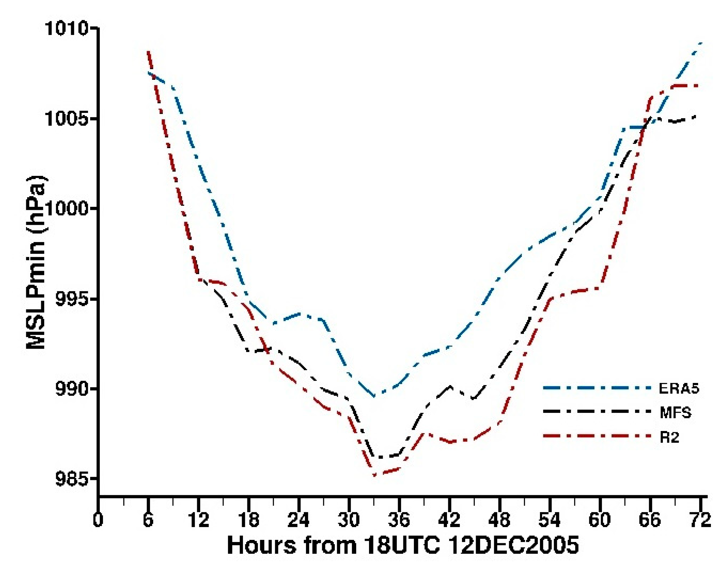
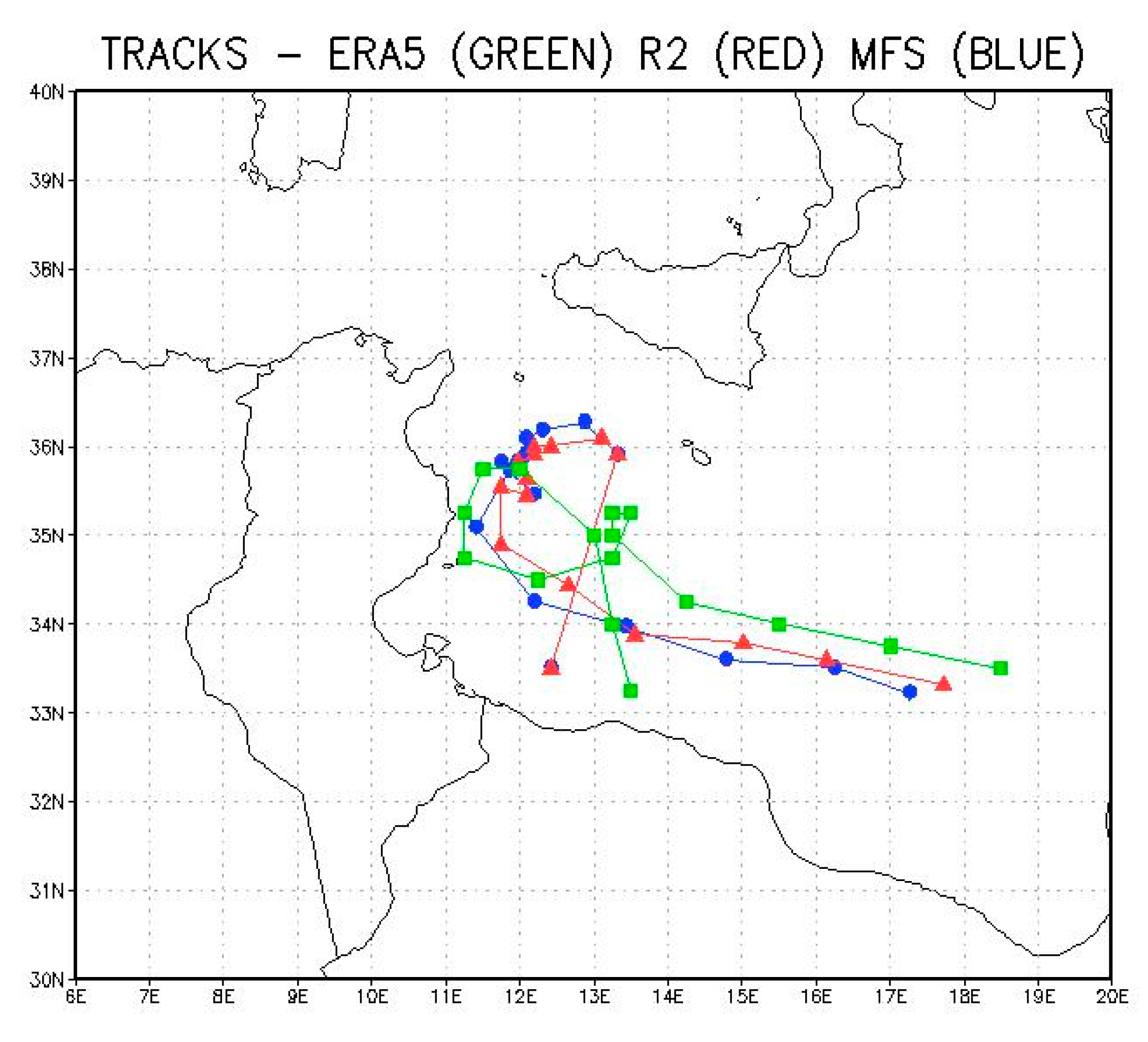
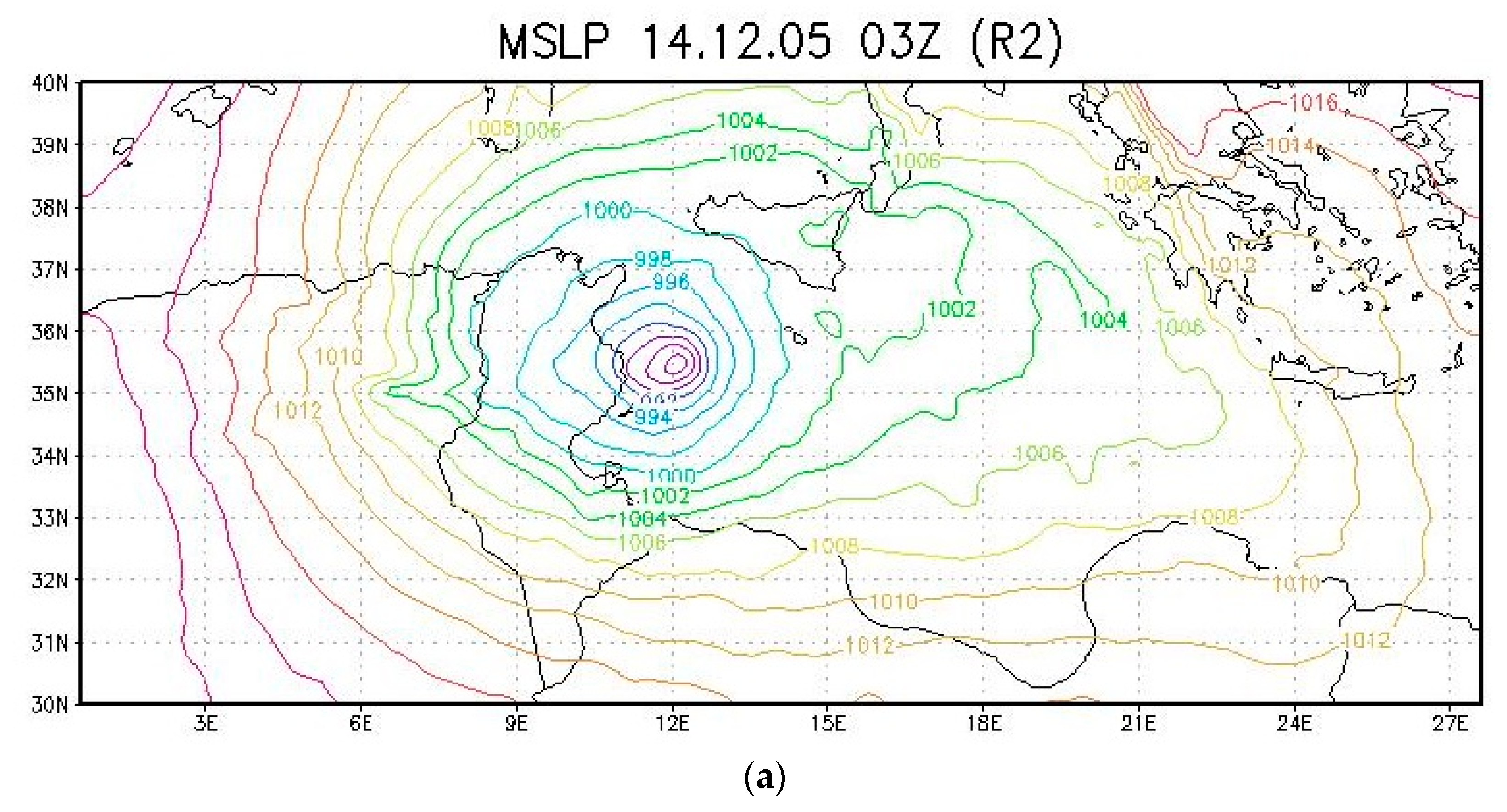
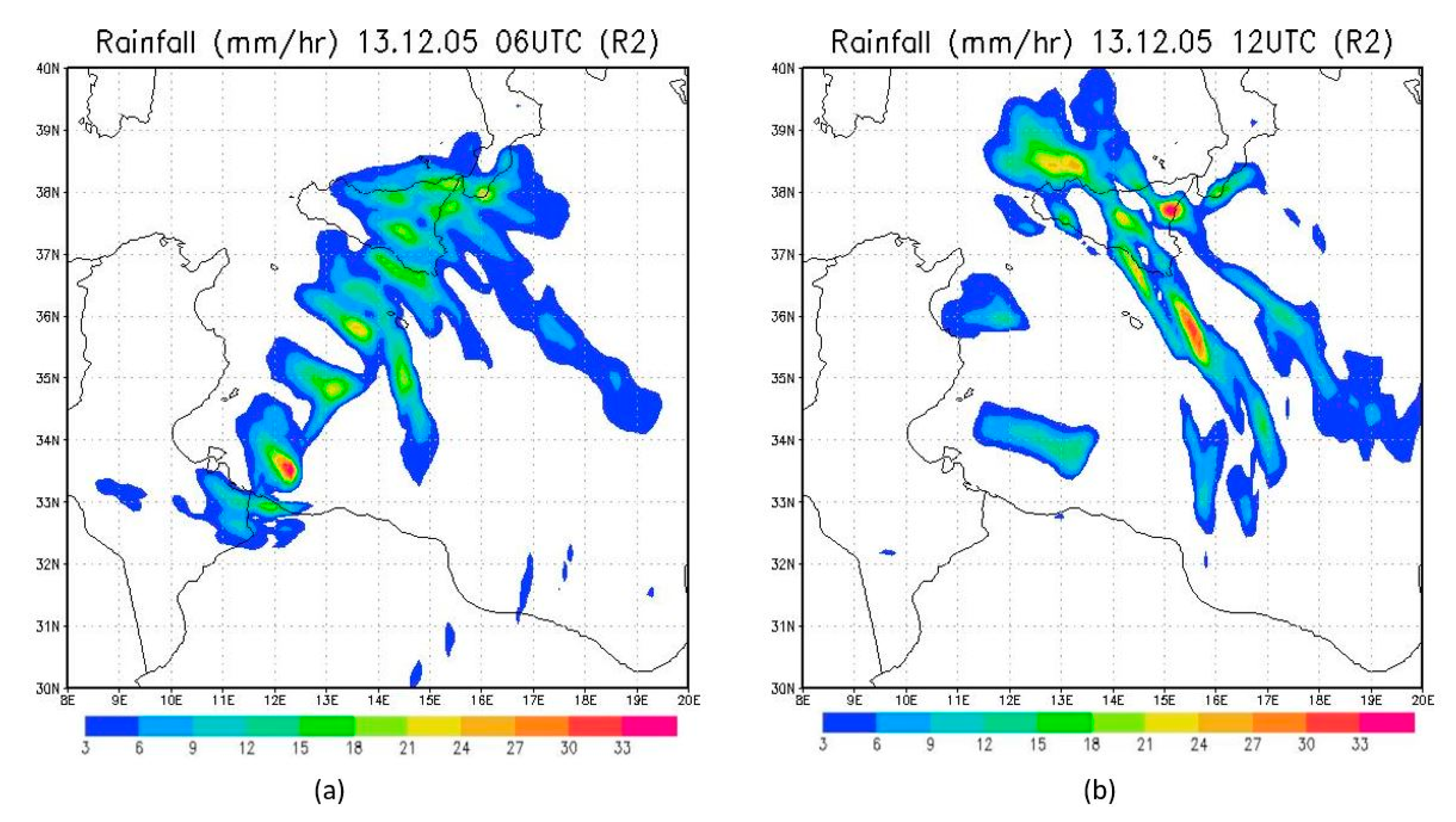
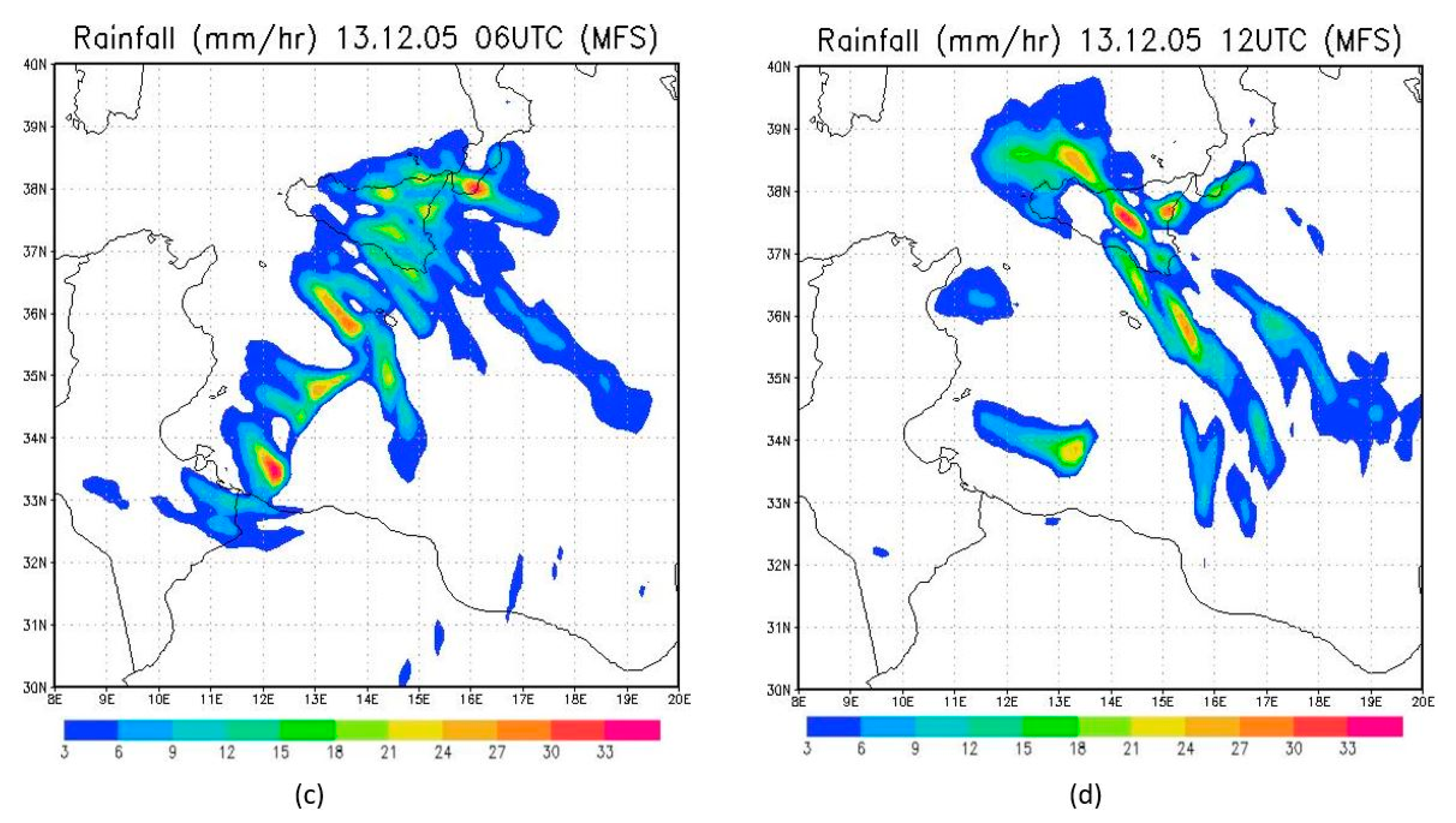
4.1. Results for the TLC of December 2005

4.1.1. The TLC R2 and MFS Simulations

Both the R2 and MFS simulations were initialized on 12 December 2005 18 UTC. The lowest surface pressure in the center of the storm was reached 33 h later at 03 UTC on 14 December 2005. The R2 and MFS SST fields for 13 December 2005 over the full model domain are shown in Figure 10a,b, respectively. The most noticeable difference is the smooth appearance of the R2 field due to its much lower resolution. The average SST south of Sicily and up to the coasts of Tunisia and Libya is 0.15 °C warmer in the R2 data as compared to MFS. Over the Gulf of Gabès (off the coast of Tunisia) where the TLC initially intensifies, the MFS SST is as much as 2 °C cooler than R2. This also occurs along the southern coast of Sicily.
A comparison of the evolution of the central MSLP in the TLC for the ERA5 reanalysis and the two simulations is shown in Figure 11. The pattern of intensification and weakening of the storm as well as the timing of the peak of storm were properly captured in both model runs. The simulated minimum MSLP in both model runs was deeper than the reanalysis values throughout the entire period, probably due to the higher resolution of the model (10 km compared to ~25 km for the reanalysis). Most of the time the R2 minimum MSLP was slightly lower than the MFS value, suggesting that the higher SST in R2 led to a somewhat more intense storm. The central MSLP values at the peak of the storm were 989.6, 985.2 and 986.1 hPa for ERA5, R2 and MFS, respectively.
The storm tracks from both simulations for the period from 13 December 2005 00 UTC to 15 December 2005 00 UTC are shown in Figure 12. Since the shape of the TLC is fairly well defined, the track was determined by scanning for the lowest MSLP within a predefined ~600 km × 500 km box at each time step. The storm initially formed and remained nearly stationary over the southern Gulf of Gabès. It then moved northwestward towards the center of the Sicily channel where rapidly intensified and reached its peak between 03–06 UTC on 14 December 2005. As the storm slowly weakened it tracked southward back towards the Gulf of Gabès and then turned eastward towards the central Mediterranean. For comparison the track computed from the (coarser resolution) ERA5 reanalysis is shown. The main difference between the simulated and the reanalysis tracks occur during the early stage of intensification when the simulated TLCs move further north than observed. During the weakening phase the two simulated tracks are located slightly south of the reanalysis track. The mean track errors during the 18 h prior to the peak of the storm are 100 km and 103 km, respectively for the R2 and MFS runs. These values are somewhat higher than the mean values, but within the range of errors, obtained in other studies of TLCs which focused on better initialization of nowcasts [16] or various combinations of subgrid scale parameterizations [17,18]. During the intensification phase, the two simulated tracks were very similar with a mean difference of 13 km. They start to diverge after the peak of the storm with the R2 track generally located to the east-northeast of the MFS track. The largest difference between the tracks appeared during the six hours following the peak with values of up to 45 km.
The MSLP maps for the R2 and MFS simulations at the peak of the TLC on 14 December 2005 03 UTC are shown in Figure 13. At this time the center of the TLC in the MFS run was located about 10 km to the east of the R2 center while the R2 central pressure was 0.9 hPa lower.
The most intense rainfall occurred the day before the peak of the storm, between 06–12 UTC 13 December 2005 as shown in the TRMM data in Figure 4. The corresponding model results (3 h accumulated rainfall expressed in units of mm h−1) for both model runs are shown in Figure 14. The general pattern, location and maximum rainfall rates over Sicily are reproduced reasonably well by the model although the precipitation appears is narrower bands as compared to the TRMM data. This may be partially due to the higher resolution of the model (10 km) compared to the TRMM fields (25 km).
At the peak of the storm, the simulated 10m winds from the R2 and MFS results (Figure 15) show the most intense winds of more than 20 m s−1 along the southern flank of the low, in agreement with the reanalysis field shown above in Figure 5.
Figure 16 shows the latent and sensible heat flux at the peak of the storm. The highest value appears in the south corner of the basin along the coat of Libya. The R2 values in this area are ~15% higher than MFS values due to the higher R2 SST and slightly stronger winds in this region. This together with the lower MSLP in the R2 run suggest that the air-sea interaction through the surface turbulent heat flux is important for the intensification of the TLC.

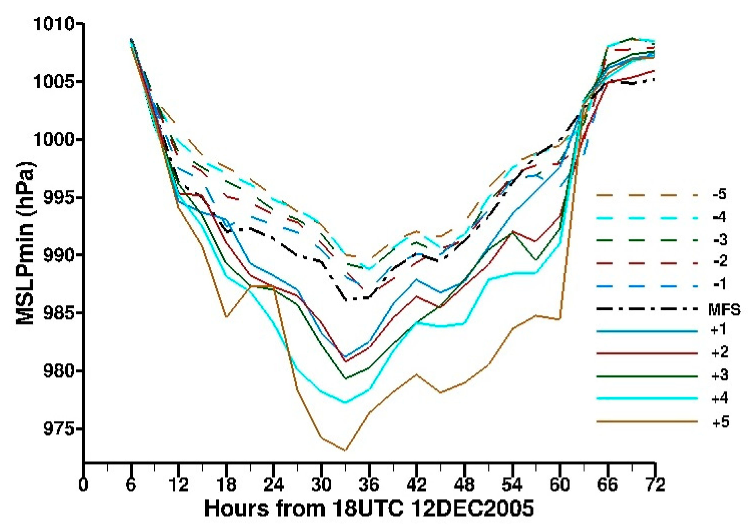
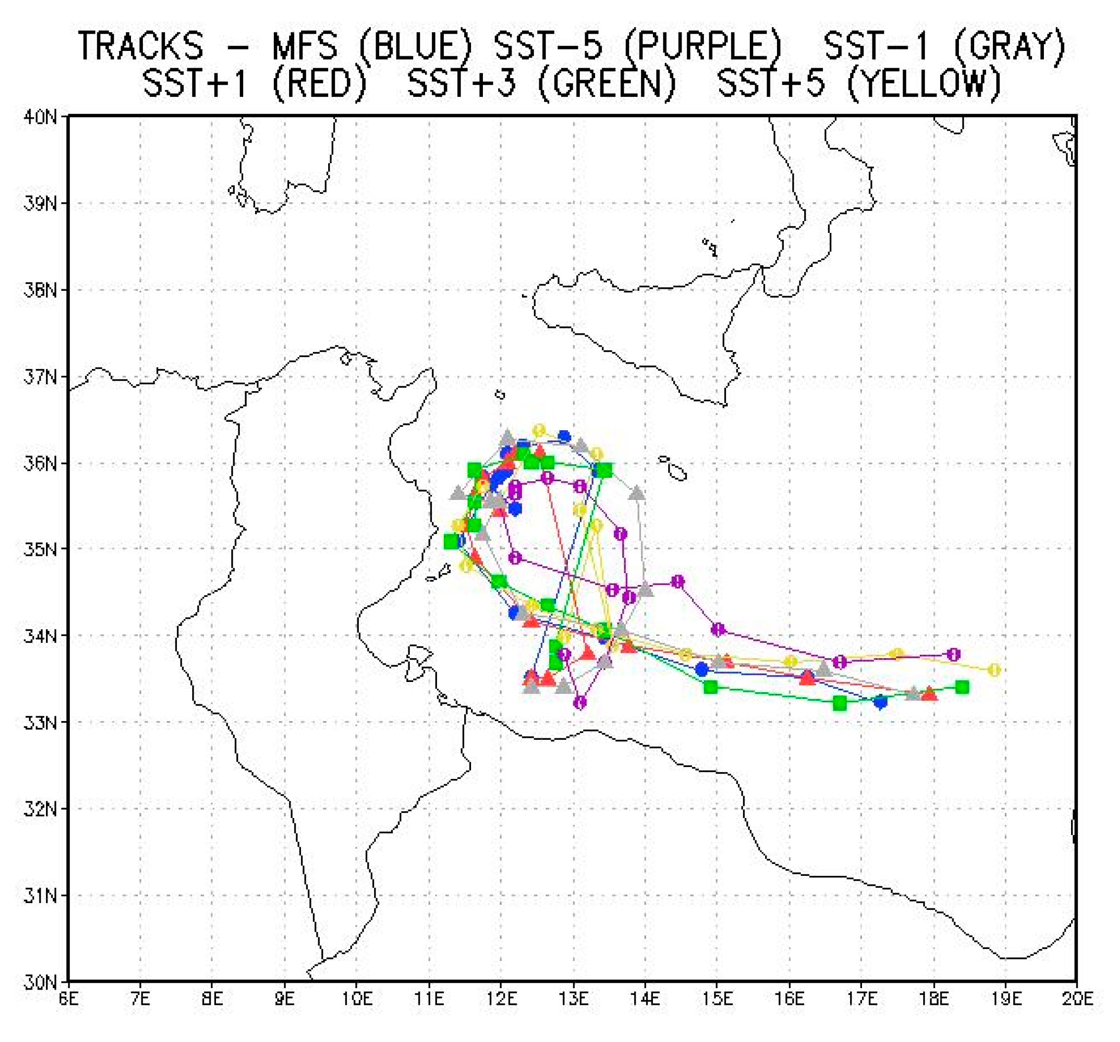
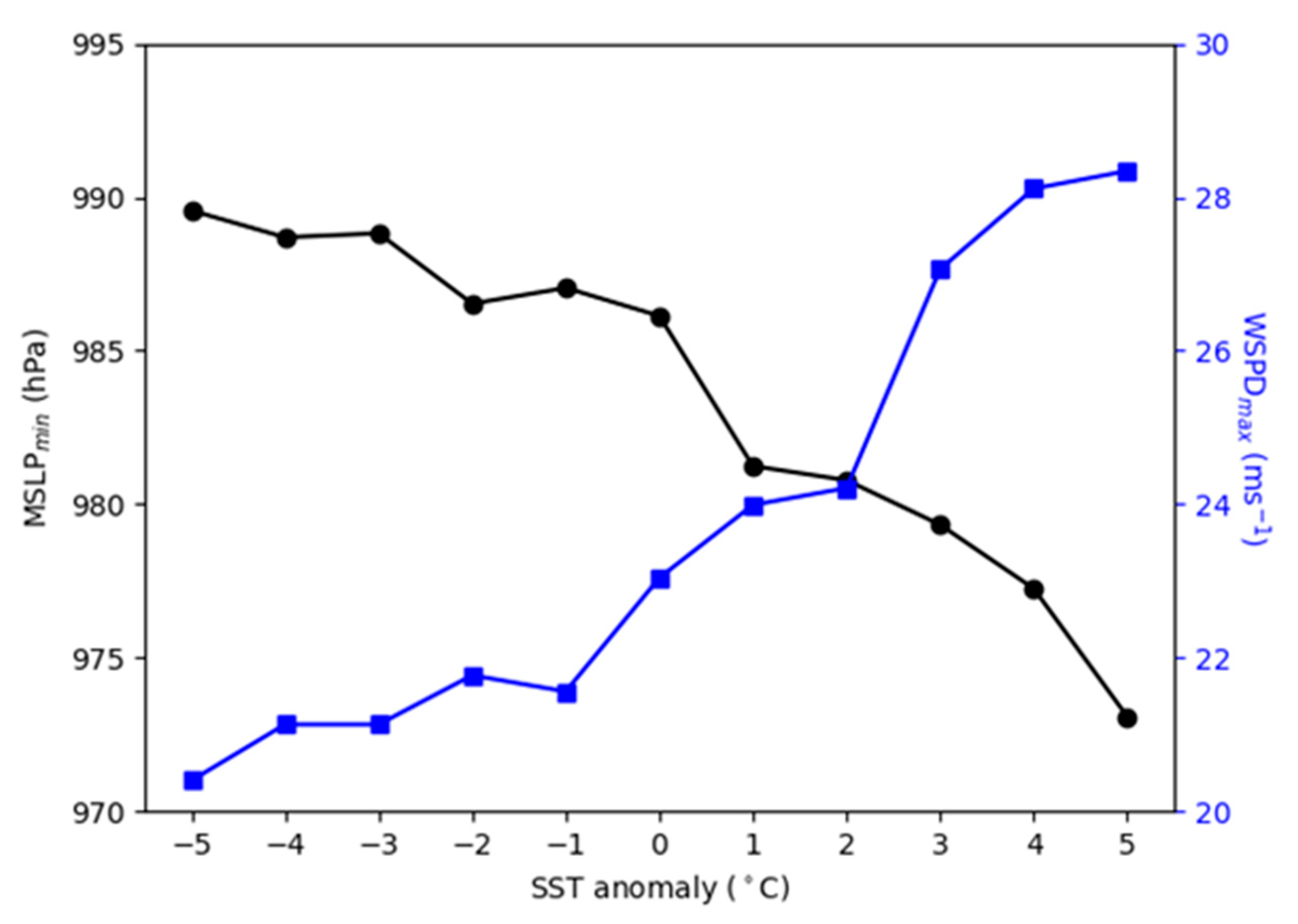
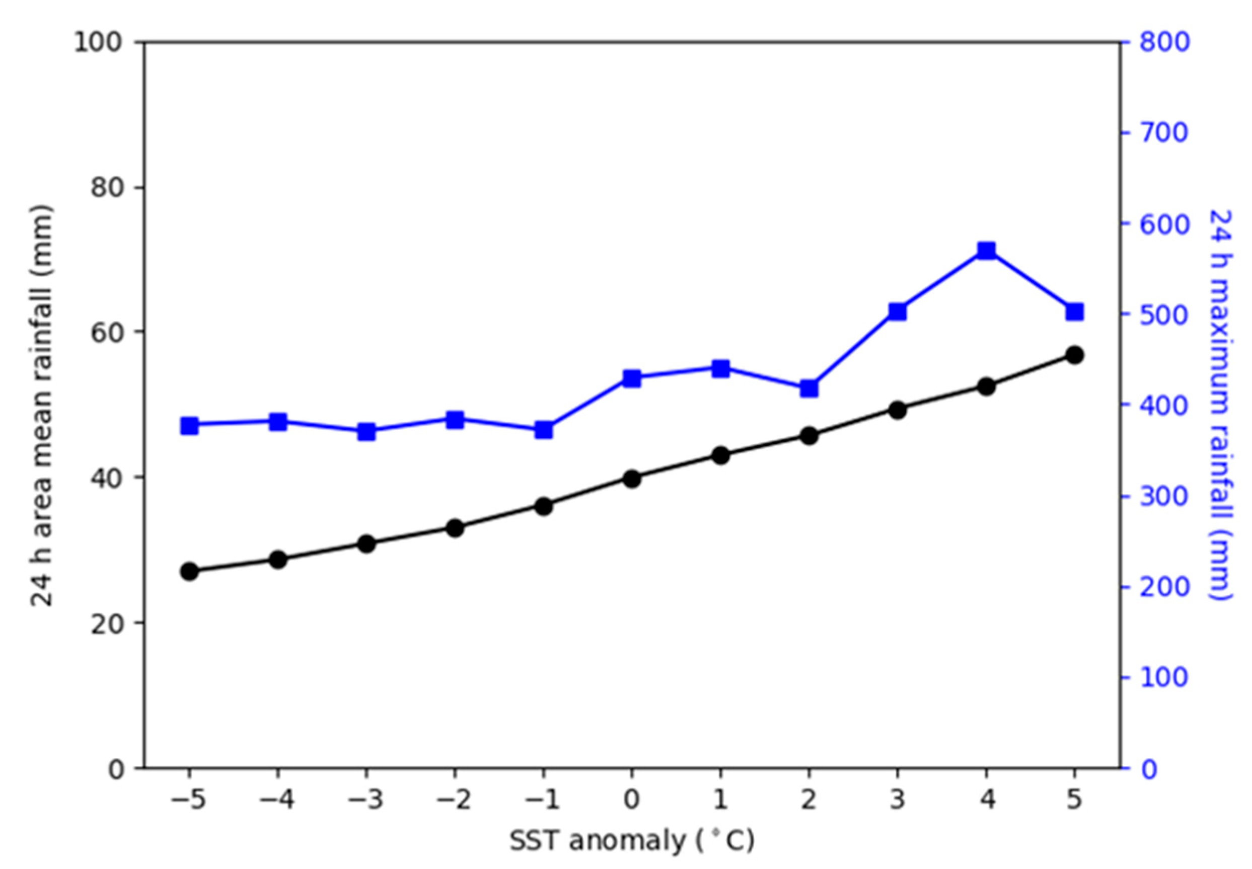
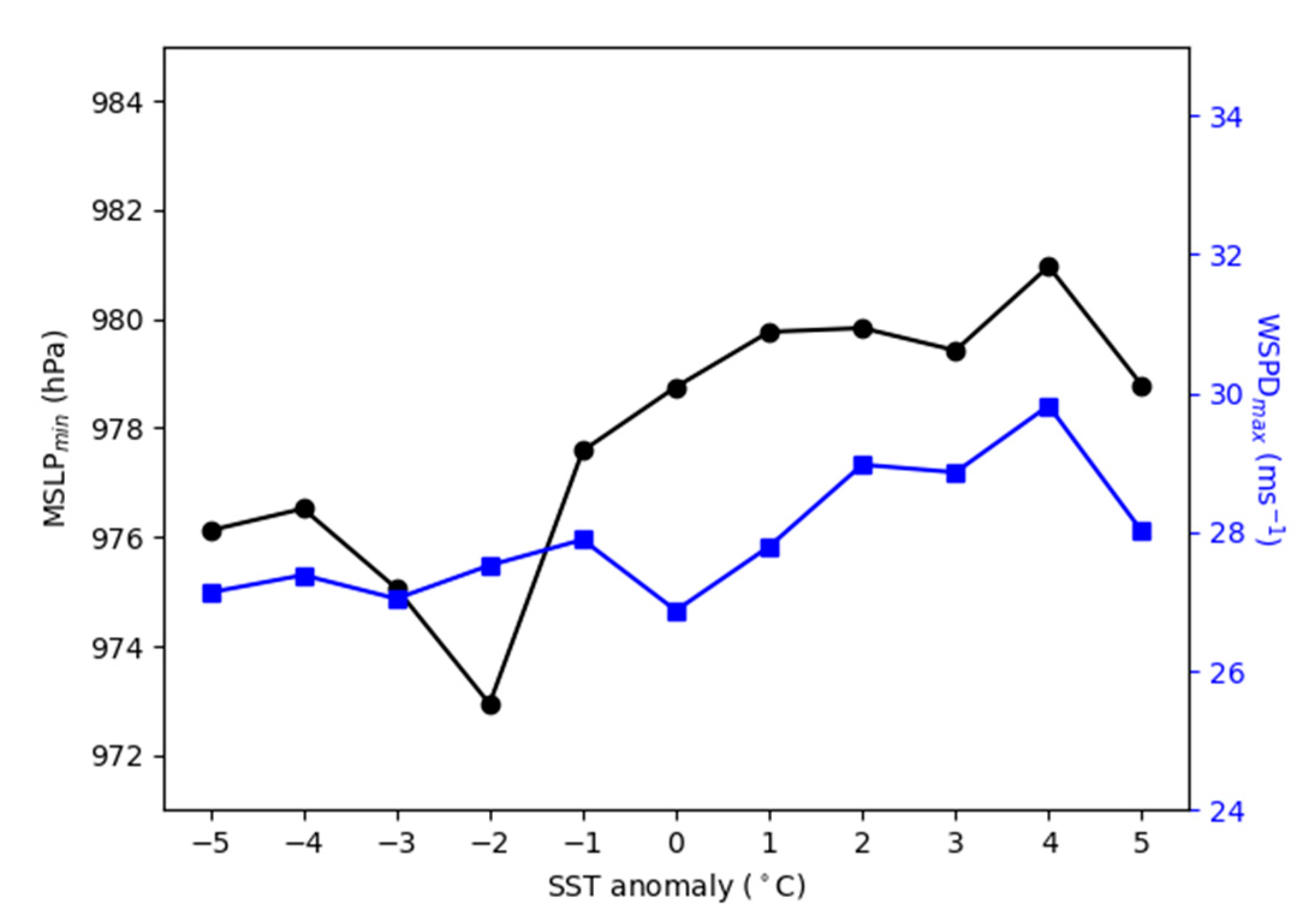
4.1.2. Sensitivity of the TLC to SST Anomalies

In response to global climate change, it is also likely that the temperature of the upper layer of the Mediterranean Sea will change accordingly. Under present conditions the SST has warmed since the early 1980’s [13] and this trend is expected to continue. The SST anomaly sensitivity experiments were therefore intended to assess the impact of this warming trend on the intensity of the TLC. We therefore ran a series of simulations with the MFS SST field increased by 1 °C increments up to a maximum increase of 5 °C. For completeness we ran an additional set of simulations for comparable SST cooling scenarios.
The time series of the minimum MSLP for the MFS and 10 SST anomaly experiments are shown in Figure 17. As expected, for warmer SSTs the storm intensifies (minimum MSLP is lower) while for cooler SSTs the storm weakens (higher minimum MSLP). We note that throughout the intensification and weakening phases the surface cooling has less of an impact, per degree change, on the intensity of the storm than for surface warming, as seen in the smaller spread of the cooling runs (dashed lines) compared to the spread of the warming runs (solid lines). The decrease in the lowest MSLP ranges from 981.2 hPa for +1 °C to 973.1 hPa for +5 °C. For the cooling runs, the increase in the lowest MSLP ranges from 986.5–990.1 hPa for −2 °C and −5 °C, respectively. The timing of the peak of the storm is not affected by warming SSTs but it is slightly delayed by up to 3 h in the cooling cases.
The storm tracks for the MFS run and for selected cool and warm SST anomalies (−5, −1, +1, +3, +5) are shown in Figure 18. During the intensification and dissipation phases there is very little difference between the MFS track and the warm anomaly simulations. During the early phases of the cyclone development, the TLC tracks further to the east and north (gray and purple tracks) in the cool anomaly runs as compared to the other runs. The most noticeable difference is in track for the most extreme cool anomaly (SST-5, purple track). In this case, the radius of the loop that the cyclone center follows during the early development and intensification phases is smaller than for the other anomalies. In addition, during the dissipation phase, as the TLC moves to the east, this track is located as much as 20–40 km north of the other tracks.
Figure 19 shows the minimum MSLP and the maximum 10 m wind speed plot at the peak of the storm (14 December 2005 03 UTC) for the MFS and all of the SST anomaly experiments. The strongest winds occur along the southern flank of the medicane (Figure 15) with the maximum wind located ~150 km from the center of the low. The MSLP curve emphasizes that the impact of SST change per degree on the intensity of the storm is significantly larger for warming (2.6 hPa/°C) than for cooling (0.7 hPa/°C). A similar trend can be seen in the maximum wind speed with changes of 1.0 m s−1/°C and 0.5 m s−1/°C for warming and cooling, respectively.
Figure 20 shows the 24 h accumulated precipitation ending at the time of the peak of the storm (14 December 2005 03 UTC) for all of the SST anomaly experiments. The black line is the spatial mean over the box bounded by 10°E–20°E and 30°N–39°N, while the blue line is the maximum value in the same domain. The trend of the increase in the area mean precipitation is nearly linear with a slope of 2.98 mm/°C. However, the impact on the maximum accumulated rainfall is quite different. The maximum rainfall for all of the cooler SST experiments is insensitive to the SST anomaly. Similarly for the warming experiments up to +2 °C the change in the maximum rainfall is negligible. There is a noticeable increase in the maximum rainfall only for SST anomalies of +3 °C or more.
The 24 h mean surface turbulent heat flux (latent + sensible) centered at the peak of the storm, averaged over the Gulf of Gabès and the Sicily channel, for all experiments as shown in Figure 21 together with the minimum MSLP indicates the importance of the heat flux for storm intensification. The linear trend (61 Wm−2/°C) together with the trend seen in the area mean rainfall suggests that the combined effects of local evaporation and heating from below over the sea contribute directly to the precipitation, although the evaporation is the dominant effect since the sensible heat flux never exceeds 30% of the latent heat flux over this region.

4.2. Results for the Explosive Cyclone of December 2010

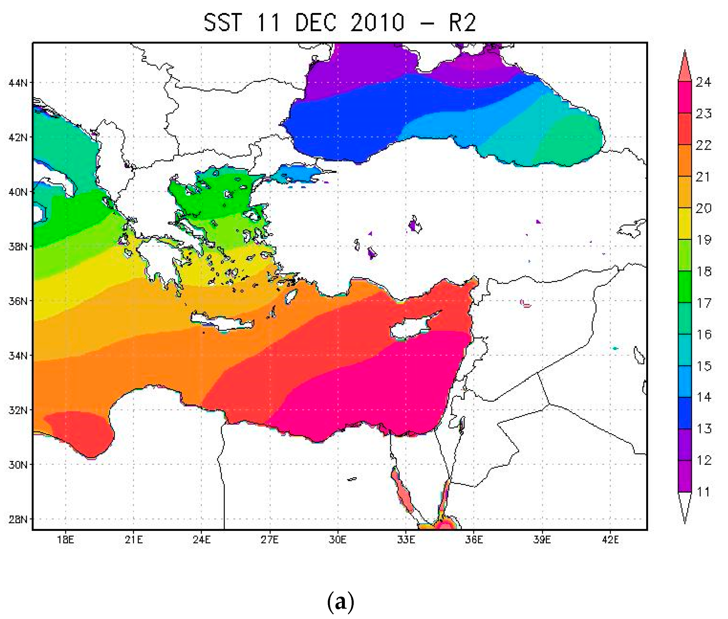
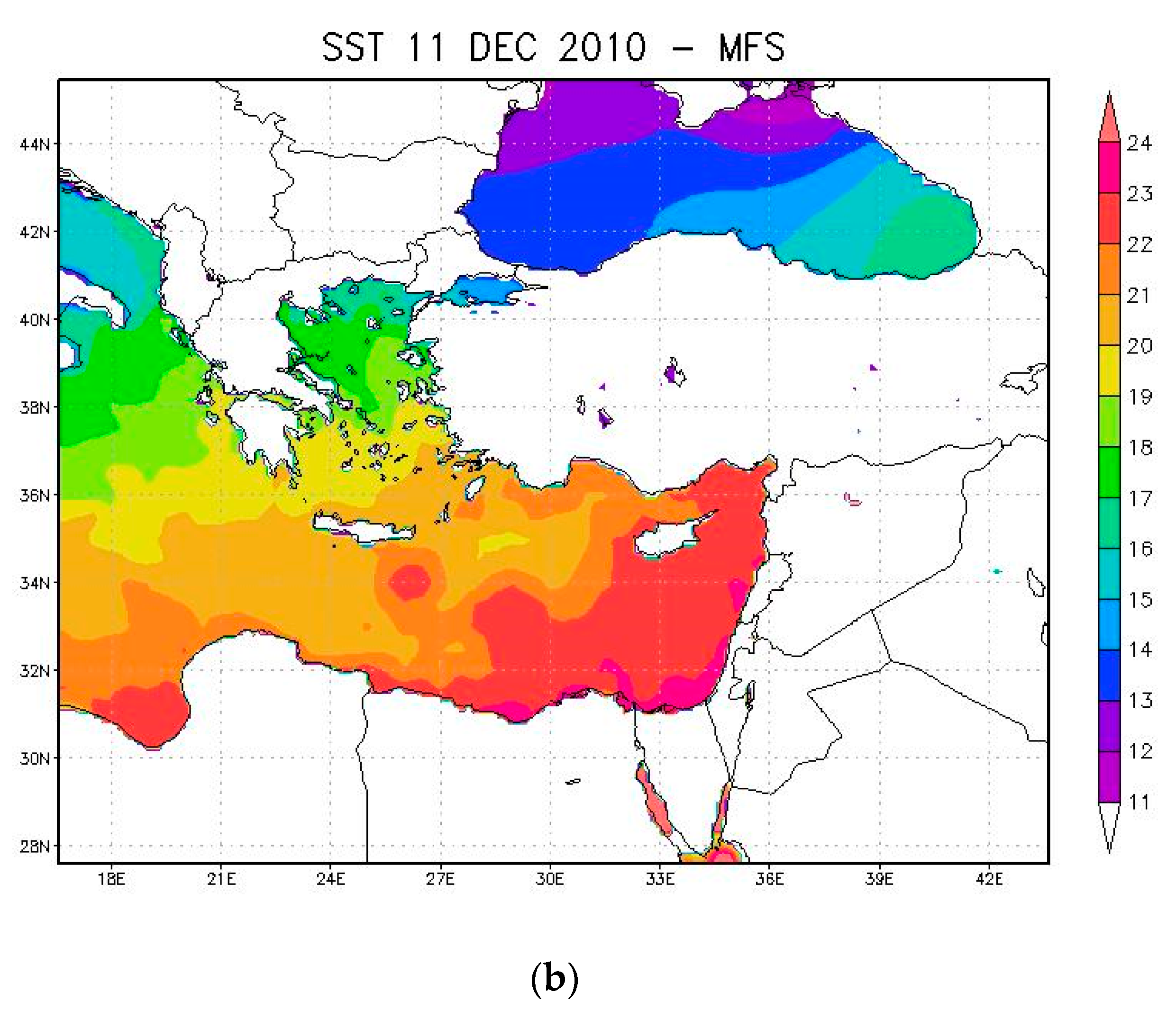
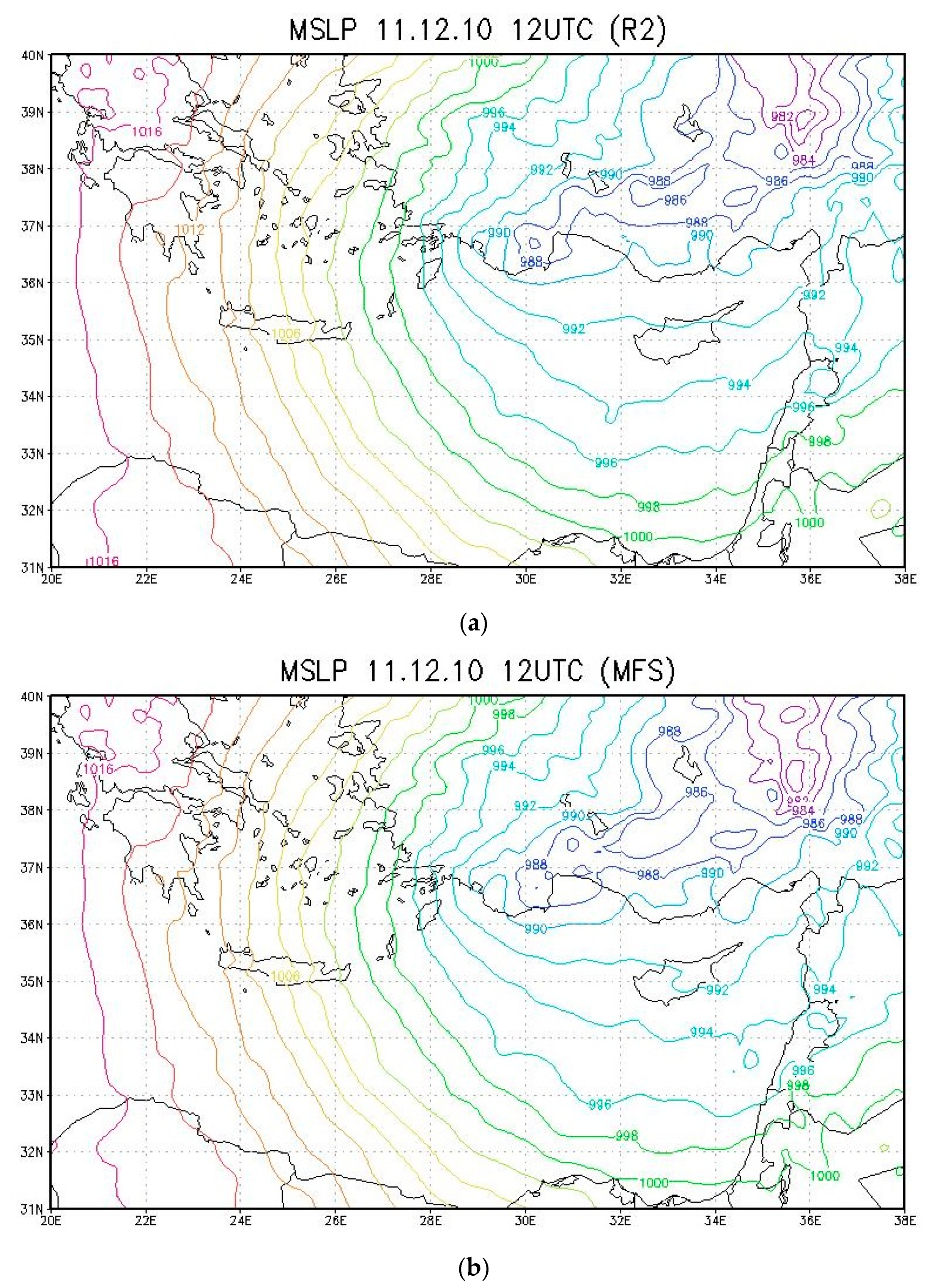
4.2.1. The Explosive Cyclone R2 and MFS Simulations

Both the R2 and MFS simulations were initialized on 10 December 2010 00 UTC. The lowest surface pressure in the center of the storm was reached 33–36 h later. The R2 and MFS SST fields for 11 December 2010 are shown in Figure 22a,b, respectively. A very noticeable patch of warm SST, referred to as the Ierapetra gyre, appears to the south/southeast of Crete in the MFS field. This feature is absent in the R2 SST field. With the exception of this region, the rest of the Levantine and Aegean seas are cooler in the MFS field. The average SST difference over the entire domain is −0.68 °C. Over the Aegean were the storm initially forms, the difference is only −0.08 °C.
The MSLP maps at the peak of the simulated storm (lowest MSLP over Turkey) on 11 December 2010 12 UTC, are shown in Figure 23 with R2 (Figure 23a) and MFS (Figure 23b). In both cases the model successfully reproduces the surface low as an elongated band stretching from the Gulf of Antalya to the northeast over Turkey, almost reaching the Black Sea. The two low centers in this band, one over the Gulf of Antalya and one to the northeast over Turkey were also reproduced by the model, although the model maintained the latter low (primary) as the deeper of the two. The minimum MSLP values for the primary low over Turkey were 978.8 and 979.2 for MFS and R2, respectively. At this hour, however, the ERA reanalysis showed the secondary low as the deeper of the two with a minimum MSLP of 986.7 hPa. The ERA reanalysis showed the low over Turkey as having reached is lowest value of 986.5 hPa nine hours earlier. During the following six hours the low over Turkey weakens in the RSM and the secondary low becomes the dominant system. Interestingly, an additional, short-lived secondary low appeared between northeast Cyprus and the Gulf of Iskenderun three hours earlier (11 December 2010 09 UTC) with a closed 986 hPa isobar in the R2 run and as a narrow trough in the MFS run (maps not shown).
The time series plots of MSLP accounting for both the primary and secondary lows (over the Gulf of Antalya and near the Gulf of Iskenderun) for the ERA5 reanalysis, the R2 and the MFS runs from the storm’s formation to decay are shown in Figure 24. The model clearly favored the development of the primary low over Turkey while the ERA5 reanalysis showed that the intensities of the land based low and the secondary low over the Gulf of Antanlya were comparable (minimum MSLPs of 986.5 and 986.7 hPa, respectively) with the secondary low appearing 9 h later than the primary low. These two lows appear as relative minima in blue line of Figure 24 at 27 and 36 h, respectively. In both model runs, however, the low over Turkey is the main center of action. The difference of only 0.4 hPa between the two model simulations does not appear to be significant.
The 12 h accumulated rainfall maps during the explosive cyclogenesis phase are shown in Figure 25 for the R2 (left panel) and the MFS (right) simulations. The patterns and amounts are very similar in both the R2 and MFS runs. The maximum R2 rainfall is only 1 mm more than the MFS value. The region of the heaviest rainfall appears over the northeast corner of the Levantine basin. This location and the amounts are consistent with the analyzed TRMM values shown above in Figure 8. However, in contrast to the TRMM data, the rainfall in the model is separated into several narrower, elongated bands that extend to the west and to the south. This is most likely due to the higher resolution of the model (10 km as compared to ~25 km for TRMM). This was confirmed by a single model run with a 25 km horizontal grid in which the elongated, narrow precipitation bands merged into a larger patch, more similar in appearance to the TRMM rainfall map shown above in Figure 8 (results not shown).
The strongest 10 m winds, which occur 3 h before the peak of the storm, are shown in Figure 26. A broad zone of strong winds with speeds over 18 m s−1 appears along the southern flank of the storm, across the southern half of the Levantine basin with maximum values of over 20 m s−1 off the coast of Egypt. However, the strongest winds occur in the northeastern corner of the Levantine basin in a narrow band extending southward along the coasts of Syria and Lebanon. The speeds exceed 24 m s−1. The differences between the R2 and MFS simulated winds were minimal.
Finally, the turbulent heat flux (latent + sensible) over the sea at the peak of the simulated storm is shown in Figure 27. The highest values of over 1000 Wm−2 appear in the western Levantine basin covering the area between Crete and the coasts of Egypt and Libya. There are also several patches of high heat flux over the southern and northeastern Aegean Sea. The sensible heat flux accounts for less than 30% of the total turbulent heat flux across the Levantine basin, and for 30–40% of the total flux across the Aegean Sea. The R2 run shows slightly higher values than MFS run with a larger area covered by values over 1100 Wm−2.

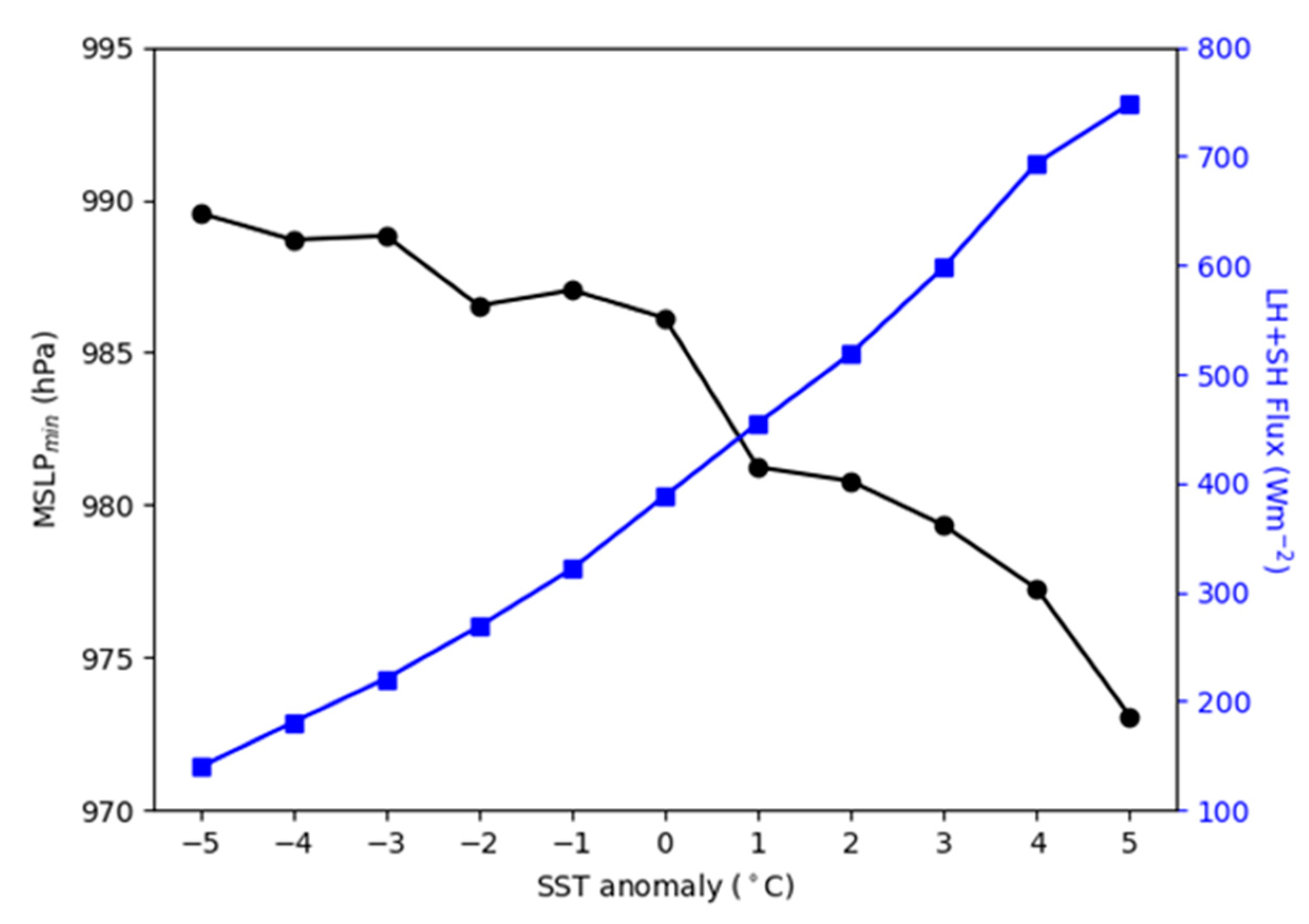
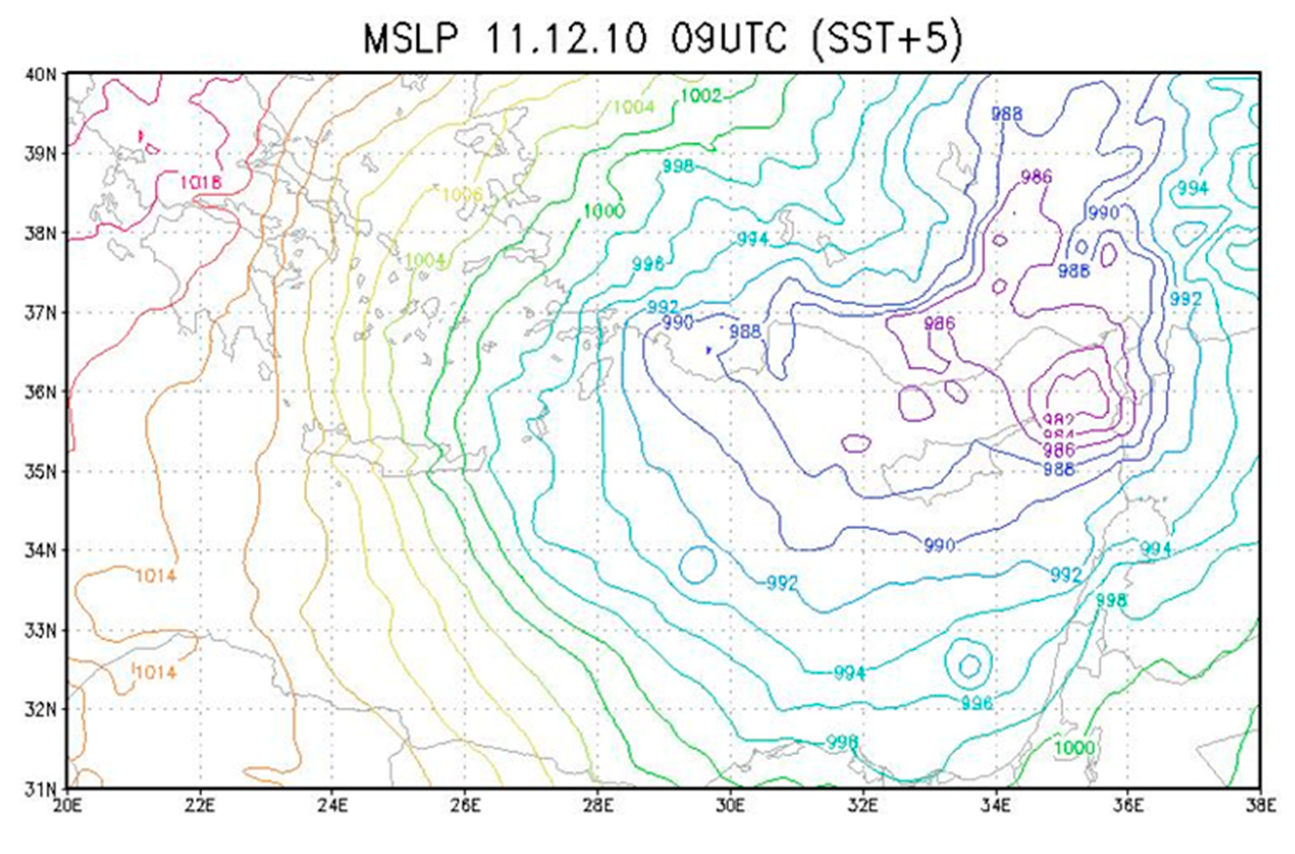
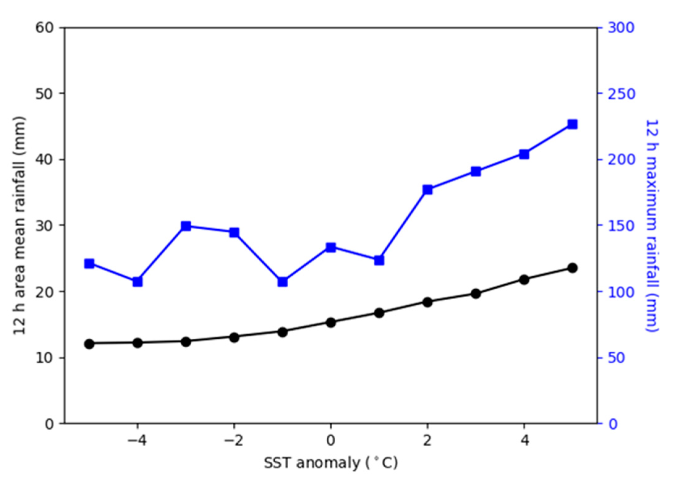
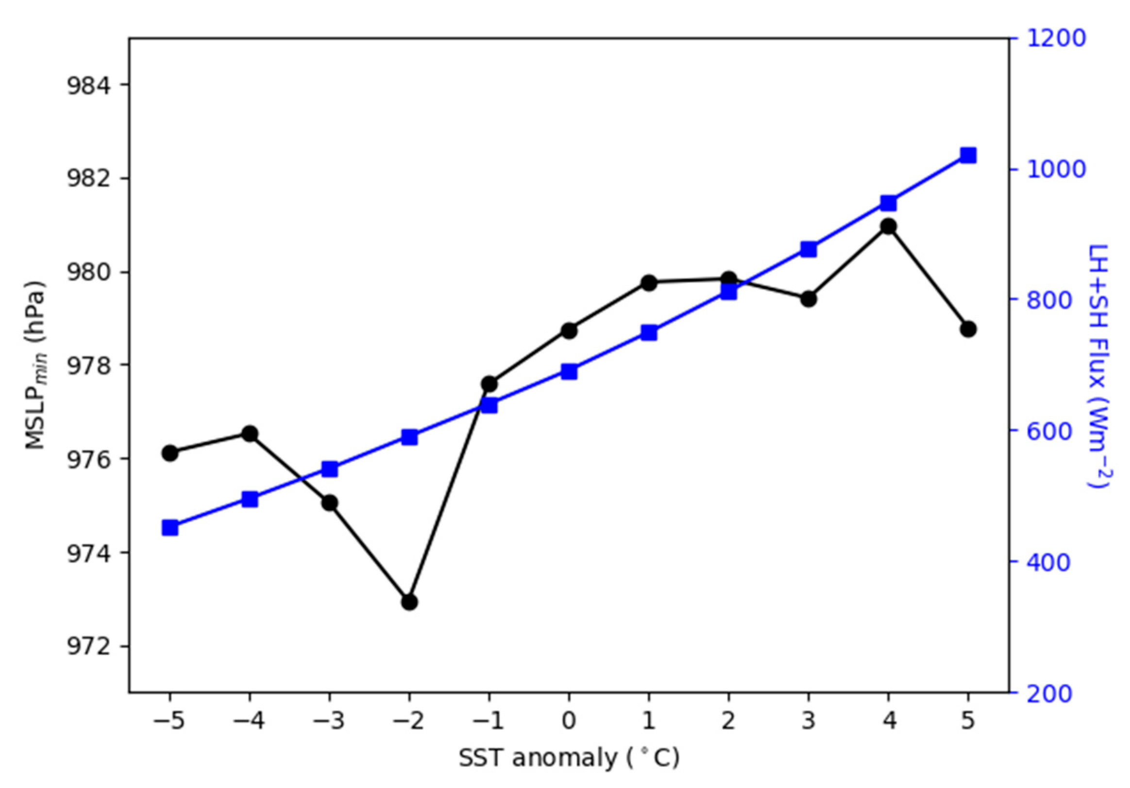
4.2.2. Sensitivity of the Explosive Cyclone to SST Anomalies

As in the case of the TLC, here too we were interested in the sensitivity of explosive cyclogenesis to the warming trend observed in the SST of the Mediterranean [13] and the projected continued warming [31]. We therefore also ran a series of simulations with the MFS SST field increased by 1 °C increments up to a maximum increase of 5 °C, and for completeness we ran an additional set of simulations for comparable SST cooling scenarios.
The sensitivity of the storm’s intensity, as indicated by the minimum MSLP time series plot in Figure 28, is quite different than for the TLC case. Here the impact of increasing SST appears to have only a minimal effect as indicated by the small spread of the five positive SST anomaly experiments (solid lines). For the cooling experiments there is some intensification of the storm, but this is mainly seen for the −2 °C and −3 °C experiments. The lack of a consistent or significant trend in the minimum MSLP as a function of the SST anomaly is further emphasized by the black line shown in Figure 29. If we consider the maximum wind speed over the entire extent of the low at 3 h before the peak of the storm (lowest MSLP) as an indication of the storm’s intensity, as shown by the blue line in Figure 29, we find negligible sensitivity for the cooling experiments but an increasing trend of +0.74 m s−1/°C for the warm SST anomalies up to 4 °C which is less than TLC case (+1 m s−1/°C). One interesting is a shift in the location of the secondary low for SST anomalies of 3 °C or more. For these experiments, a short-lived (<12 h duration) secondary low develops between northeast Cyprus and the Gulf of Iskenderun, with minimum MSLP values lower than the Gulf of Antalya low, which appears as a weak trough. As an example, the MSLP field for the +5 °C SST anomaly is shown in Figure 30 where the noticeable eastward shift in the location of this short-lived secondary can be seen. In fact, it disappeared three hours later with the primary low over Turkey being the dominant low-pressure center.
Figure 31 shows the 12 h accumulated precipitation during the explosive cyclogenesis phase from 10 December 2010 18 UTC until 11 December 2010 06 UTC. The black line is the area mean over the box bounded by 26–36°E and 33–38°N, while the blue line shows the maximum. The area mean rainfall increases over the entire range of SST anomalies with a slope of 1.15 mm/°C. In contrast to this, the response of the maximum rainfall for the cool anomalies is variable with no consistent trend. However, for the warm anomalies it increases at a rate of 18.6 mm/°C.
We conclude with Figure 32 which shows the sensitivity of the turbulent heat flux (latent + sensible) at the sea surface averaged over the Levantine basin at the peak of the storm (blue line), and the sensitivity of the minimum MSLP (black line) which accounts for the location shift of the secondary low to the northeastern corner of the basin for the highest SST anomalies, as noted above. Not surprisingly, the turbulent heat flux shows a smooth nearly linear increase across the entire range of SST anomalies. As for the minimum MSLP, we now see that by accounting for the significant shift in the location of the development of secondary low from the Gulf of Antalya eastward to the Gulf of Iskenderun, the low over the sea does indeed intensify and deepen for SST anomalies greater than 2 °C.

5. Discussion and Conclusions

In this study, our goal was to examine the sensitivity of simulations of a TLC (December 2005) and an explosive cyclone (December 2010) over the Mediterranean to the specification of sea surface temperature (SST) by using a regional atmospheric model (RSM) with high spatial resolution SST data (MFS) compared to lower resolution data (R2). In addition, we ran a series of sensitivity experiments to assess the response of the two storms to warming and cooling of SST, the former indicative of projected changes due to global warming and the latter for completeness. The intensity of each storm was assessed by the minimum MSLP and the maximum wind speed attained, while the direct effect of sea forcing was assessed through changes in the precipitation and the surface turbulent heat fluxes over the sea.
The storm first appeared as a weak surface low over Libya on the evening of 12 December 2005. During the night it moved northward over the Gulf of Gabès and Sicily channel (SST ~19 °C) where it remained and rapidly intensified, reaching its maximum intensity (lowest MSLP) in the early morning of 14 December 2005, and by that evening it began to move to the east towards the Levantine basin where it finally dissipate on 16 December 2005. Throughout the day of 13 December 2005, a cutoff upper-level low was present over north Algeria and the adjacent sea, bringing cold air from Western Europe to the Mediterranean Sea while at lower levels warm, dry air was advected from North Africa, thereby supporting the rapid intensification of the TLC. The higher SSTs off the coasts of Tunisia and Libya in the R2 data as compared to the MFS data led to a slightly stronger TLC in the R2 simulation with a minimum MSLP that was ~1 hPa lower. Similarly, the maximum rainfall was 7% higher and the maximum turbulent heat flux was 15% higher in the R2 run as compared to the MFS run. The simulated track errors of the cyclone center compared to the ERA reanalysis were within the ranges of TLC track errors found in other, more detailed studies [17,18]. Slight differences between the R2 and MFS tracks, especially in the hours following the peak of the storm, suggest that the additional spatial details in the MFS SST contribute to the motion of the storm although when considering the overall structure of the cyclone the effect is probably minimal. In the SST anomaly experiments, the impact on the TLC was clear and consistent with all parameters (MSLP, maximum wind speed, precipitation and turbulent heat flux) pointing to an increase in the storm’s intensity as the surface temperature rises, although the effect was much more noticeable for the warm anomaly cases than for the cool anomaly cases. We also note that the peak of the storm occurs slightly earlier (~3 h) in the warm SST anomaly cases. Interestingly though, the warm SST anomalies had a minimal effect on the track of the center of the cyclone. In fact, the most pronounced effect on the track was seen in the most extreme cool anomaly case (SST-5) where the radius of the loop followed by the TLC during the early development an intensification phases was noticeably smaller than for all other tracks. Overall, these results suggest that SST plays a direct role in determining the intensity of the storm.
The explosive cyclone case of December 2010 initially formed on the night of 9–10 December 2010 as a cold trough extending southwestward from Russia over the Aegean Sea. As the storm intensified it followed an eastward/southeastward path with the cyclone center moving across Turkey and the southern flank of the storm moving across the relatively warm Levantine basin with SSTs of 20–21 °C. The development of the storm was supported by the intrusion of a cold, upper-level trough. While the storm center continued to move eastward across mainland Turkey, a secondary low developed over the Gulf of Antalya thus creating an elongated band of low pressure that extended northeastward from the Gulf of Antalya reaching almost to the Black Sea. The storm reached its peak intensity mid-day on 11 December 2010. The differences between the intensity of the cyclone in the R2 and MFS were minimal in terms of all parameters considered—minimum MSLP, maximum wind speed, rainfall and surface turbulent heat flux over the sea, even though the R2 SSTs were warmer than MFS across most of the Levantine basin. The minimal impact of the differences in the SST fields suggests that since the storm developed mainly over land, the upper-level dynamical processes such as potential vorticity anomalies and the intrusion of cold stratospheric air [13,41] are more important than direct sea surface forcing. This suggestion is further supported by the SST anomaly experiments where no clear and consistent trend is seen in the storm intensity as measured by the minimum MSLP and maximum wind speed. However, we did notice that an additional short-lived, secondary low developed in the model simulations between northeast Cyprus and the Gulf of Iskenderun. For the warm SST anomalies of +3 °C or more, this secondary low intensified significantly, but it was of limited duration (<12 h) so that the peak of the storm, as measured by the lowest MSLP attained, was still associated with the low-pressure center over Turkey. Nevertheless, the rainfall (area mean and maximum) and the turbulent surface heat flux exhibit a clear upward trend across all SST anomalies, thereby suggesting that local evaporation from the sea and destabilization due to surface warming contribute significantly to the rainfall.
The potential influence of the climate change on Mediterranean Sea SST over the coming decades is projected to warm the by 1.73–2.97 °C relative to the 1961–1990 climatology [42]. The results of our SST anomaly experiments suggest that extreme storms in the Mediterranean region will be stronger as the sea surface warms, consistently leading to increased rainfall and the potential for severe flooding. Maximum wind speeds may also be expected to increase as the SST warms, especially in storms such as TLCs that develop mainly over the sea, assuming that upper air conditions remain unchanged.

Author Contributions

This research is a central component of O.H.’s M.Sc. thesis. Conceptualization, S.B. and O.H.; methodology, S.B. and O.H.; simulations, O.H.; validation, O.H.; formal analysis, O.H. and S.B.; writing—original draft preparation, O.H.; writing—review and editing, S.B.; supervision, S.B. All authors have read and agreed to the published version of the manuscript.

Funding

This research received no external funding.

Acknowledgments

We acknowledge the use of imagery from the NASA worldview application (https://worldview.earthdata.nasa.gov, accessed on 27 April 2021), part of the NASA Earth Observing System Data and Information System (EOSDIS). ERA 5 reanalysis data were generated using the Copernicus Climate Change Service Information 2020. The high-resolution SST data were generated using the Copernicus Marine Environment Monitoring Service (CMEMS). We also thank Vasu Misra and his team at COAPS/FSU for their help, advice and guidance in working with the RSM. Finally, we thank the three anonymous reviewers whose comments have helped us to significantly improve the paper.

Conflicts of Interest

The authors declare no conflict of interest.

References

  1. Michaelides, S.; Karacostas, T.; Sanchez, J.L.; Retalis, A.; Pytharoulis, I.; Homar, V.; Romero, R.; Zanis, P.; Giannakopoulos, C.; Bühl, J.; et al. Reviews and perspectives of high impact atmospheric processes in the Mediterranean. Atmos. Res. 2018, 208, 4–44. [Google Scholar] [CrossRef]
  2. Miglietta, M.M.; Moscatello, A.; Conte, D.; Mannarini, G.; Lacorata, G.; Rotunno, R. Numerical analysis of a Mediterranean ‘hurricane’ over south-eastern Italy: Sensitivity experiments to sea surface temperature. Atmos. Res. 2011, 101, 412–426. [Google Scholar] [CrossRef]
  3. Pytharoulis, I. Analysis of a Mediterranean tropical-like cyclone and its sensitivity to the sea surface temperatures. Atmos. Res. 2018, 208, 167–179. [Google Scholar] [CrossRef]
  4. Fita, L.; Romero, R.; Luque, A.; Emanuel, K.; Ramis, C. Analysis of the environments of seven Mediterranean tropical-like storms using an axisymmetric, nonhydrostatic, cloud resolving model. Nat. Hazards Earth Syst. Sci. 2007, 7, 41–56. [Google Scholar] [CrossRef]
  5. Cavicchia, L.; von Storch, H. The simulation of medicanes in a high-resolution regional climate model. Clim. Dyn. 2011, 39, 2273–2290. [Google Scholar] [CrossRef]
  6. Lolis, C.J.; Bartzokas, A.; Katsoulis, B.D. Relation between sensible and latent heat fluxes in the Mediterranean and precipitation in the Greek area during winter. Int. J. Clim. 2004, 24, 1803–1816. [Google Scholar] [CrossRef]
  7. Tous, M.; Romero, R. Meteorological environments associated with medicane development. Int. J. Clim. 2012, 33, 1–14. [Google Scholar] [CrossRef]
  8. Nastos, P.; Papadimou, K.K.; Matsangouras, I. Mediterranean tropical-like cyclones: Impacts and composite daily means and anomalies of synoptic patterns. Atmos. Res. 2018, 208, 156–166. [Google Scholar] [CrossRef]
  9. Fita, L.; Flaounas, E. Medicanes as subtropical cyclones: The December 2005 case from the perspective of surface pressure tendency diagnostics and atmospheric water budget. Q. J. R. Meteorol. Soc. 2018, 144, 1028–1044. [Google Scholar] [CrossRef]
  10. Kouroutzoglou, J.; Avgoustoglou, E.N.; Flocas, H.A.; Hatzaki, M.; Skrimizeas, P.; Keay, K. Assessment of the role of sea surface fluxes on eastern Mediterranean explosive cyclogenesis with the aid of the limited-area model COSMO.GR. Atmos. Res. 2018, 208, 132–147. [Google Scholar] [CrossRef]
  11. Black, M.T.; Pezza, A.B. A universal, broad-environment energy conversion signature of explosive cyclones. Geophys. Res. Lett. 2013, 40, 452–457. [Google Scholar] [CrossRef]
  12. Sanders, F.; Gyakum, J.R. Synoptic-Dynamic Climatology of the “Bomb”. Mon. Weather. Rev. 1980, 108, 1589–1606. [Google Scholar] [CrossRef] [Green Version]
  13. Kouroutzoglou, J.; Flocas, H.A.; Keay, K.; Simmonds, I.; Hatzaki, M. On the vertical structure of Mediterranean explosive cyclones. Theor. Appl. Clim. 2012, 110, 155–176. [Google Scholar] [CrossRef]
  14. Pastor, F.; Valiente, J.A.; Palau, J.L. Sea Surface Temperature in the Mediterranean: Trends and Spatial Patterns (1982–2016). Pure Appl. Geophys. 2017, 175, 4017–4029. [Google Scholar] [CrossRef] [Green Version]
  15. Ricchi, A.; Miglietta, M.M.; Bonaldo, D.; Cioni, G.; Rizza, U.; Carniel, S. Multi-Physics Ensemble versus Atmosphere–Ocean Coupled Model Simulations for a Tropical-Like Cyclone in the Mediterranean Sea. Atmosphere 2019, 10, 202. [Google Scholar] [CrossRef] [Green Version]
  16. Tiesi, A.; Pucillo, A.; Bonaldo, D.; Ricchi, A.; Carniel, S.; Miglietta, M.M. Initialization of WRF Model Simulations with Sentinel-1 Wind Speed for Severe Weather Events. Front. Mar. Sci. 2021, 8. [Google Scholar] [CrossRef]
  17. Miglietta, M.M.; Mastrangelo, D.; Conte, D. Influence of physics parameterization schemes on the simulation of a tropical-like cyclone in the Mediterranean Sea. Atmos. Res. 2015, 153, 360–375. [Google Scholar] [CrossRef]
  18. Pytharoulis, I.; Kartsios, S.; Tegoulias, I.; Feidas, H.; Miglietta, M.M.; Matsangouras, I.; Karacostas, T. Sensitivity of a Mediterranean Tropical-Like Cyclone to Physical Parameterizations. Atmosphere 2018, 9, 436. [Google Scholar] [CrossRef] [Green Version]
  19. Giorgi, F. Climate Change Hot-Spots. Geophys. Res. Lett. 2006, 33, L08707. [Google Scholar] [CrossRef]
  20. Hersbach, H.; Bell, B.; Berrisford, P.; Biavati, G.; Horányi, A.; Muñoz Sabater, J.; Nicolas, J.; Peubey, C.; Radu, R.; Rozum, I.; et al. ERA Hourly Data on Single Levels from 1979 to Present. Copernicus Climate Change Service (C35) Climate Data Store (CDS). 2018. Available online: https://cds.climate.copernicus.eu/cdsapp#!/dataset/reanalysis-era5-single-levels?tab=overview (accessed on 12 October 2020).
  21. Claud, C.; Alhammoud, B.; Funatsu, B.; Chaboureau, J.-P. Mediterranean hurricanes: Large-scale environment and convective and precipitating areas from satellite microwave observations. Nat. Hazards Earth Syst. Sci. 2010, 10, 2199–2213. [Google Scholar] [CrossRef]
  22. Huffman, G.J.; Adler, R.F.; Bolvin, D.T.; Gu, G.; Nelkin, E.J.; Bowman, K.P.; Hong, Y.; Stocker, E.F.; Wolff, D.B. The TRMM multi-satellite precipitation analysis: Quasi-global, multi-year, combined-sensor precipitation estimates at fine scale. J. Hydrometeorol. 2007, 8, 38–55. [Google Scholar] [CrossRef]
  23. Shapiro, M.A.; Keyser, D. Fronts, Jet Streams and the Tropopause. In Extratropical Cyclones; Springer Science and Business Media LLC: Berlin/Heidelberg, Germany, 1990; pp. 167–191. [Google Scholar]
  24. Kanamaru, H.; Kanamitsu, M. Scale-Selective Bias Correction in a Downscaling of Global Analysis Using a Regional Model. Mon. Weather. Rev. 2007, 135, 334–350. [Google Scholar] [CrossRef]
  25. Juang, H.-M.H.; Kanamitsu, M. The NMC Nested Regional Spectral Model. Mon. Weather. Rev. 1994, 122, 3–26. [Google Scholar] [CrossRef] [Green Version]
  26. Juang, H.-M.H.; Hong, S.-Y.; Kanamitsu, M. The NCEP Regional Spectral Model: An Update. Bull. Am. Meteorol. Soc. 1997, 78, 2125–2143. [Google Scholar] [CrossRef] [Green Version]
  27. Kanamitsu, M.; Ebisuzaki, W.; Woollen, J.; Yang, S.-K.; Hnilo, J.J.; Fiorino, M.; Potter, G.L. NCEP–DOE AMIP-II Reanalysis (R-2). Bull. Am. Meteorol. Soc. 2002, 83, 1631–1644. [Google Scholar] [CrossRef]
  28. Selman, C.; Misra, V. Simulating diurnal variations over the southeastern United States. J. Geophys. Res. Atmos. 2015, 120, 180–198. [Google Scholar] [CrossRef]
  29. Nguyen, T.V.; Mai, K.V.; Nguyen, P.N.; Juang, H.-M.H.; Nguyen, D.V. Evaluation of summer monsoon climate predictions over the Indochina Peninsula using regional spectral model. Weather. Clim. Extrem. 2019, 23, 100195. [Google Scholar] [CrossRef]
  30. He, X.; Kim, H.; Kirstetter, P.-E.; Yoshimura, K.; Chang, E.-C.; Ferguson, C.R.; Erlingis, J.M.; Hong, Y.; Oki, T. The Diurnal Cycle of Precipitation in Regional Spectral Model Simulations over West Africa: Sensitivities to Resolution and Cumulus Schemes. Weather. Forecast. 2015, 30, 424–445. [Google Scholar] [CrossRef]
  31. Zong, P.; Zhu, Y.; Tang, J. Sensitivity of summer precipitation in regional spectral model simulations over eastern China to physical schemes: Daily, extreme and diurnal cycle. Int. J. Clim. 2019, 39, 4340–4357. [Google Scholar] [CrossRef]
  32. Nobre, P.; Moura, A.D.; Sun, L. Dynamical Downscaling of Seasonal Climate Prediction over Nordeste Brazil with ECHAM3 and NCEP’s Regional Spectral Models at IRI. Bull. Am. Meteorol. Soc. 2001, 82, 2787–2796. [Google Scholar] [CrossRef] [Green Version]
  33. Chou, M.-D.; Lee, K.-T. Parameterizations for the Absorption of Solar Radiation by Water Vapor and Ozone. J. Atmos. Sci. 1996, 53, 1203–1208. [Google Scholar] [CrossRef] [Green Version]
  34. Chou, M.D.; Suarez, M.J. An efficient thermal infrared radiation parameterization for use in general circulation models. In Technical Report Series on Global Modeling and Data Assimilation; NASA/TM-1994-104606; Goddard Space Flight Center: Greenbelt, MD, USA, November 1994; Volume 3, 85p. [Google Scholar]
  35. Hong, S.-Y.; Pan, H.-L. Nonlocal boundary layer vertical diffusion in a medium-range forecast model. Mon. Weather Rev. 1996, 124, 2322–2339. [Google Scholar] [CrossRef] [Green Version]
  36. Ek, M.B.; Mitchell, K.E.; Lin, Y.; Rogers, E.; Grunmann, P.; Koren, V.; Gayno, G.; Tarpley, J.D. Implementation of Noah land surface model advances in the National Centers for Environmental Prediction operational mesoscale Eta model. J. Geophys. Res. Space Phys. 2003, 108. [Google Scholar] [CrossRef]
  37. Moorthi, S.; Suarez, M.J. Relaxed Arakawa-Schubert: A parameterization of moist convection for general circula-tion models. Mon. Weather. Rev. 1992, 120, 978–1002. [Google Scholar] [CrossRef] [Green Version]
  38. Reynolds, R.W.; Smith, T.M. Improved Global Sea Surface Temperature Analyses Using Optimum Interpolation. J. Clim. 1994, 7, 929–948. [Google Scholar] [CrossRef] [Green Version]
  39. Simoncelli, S.; Fratianni, C.; Pinardi, N.; Grandi, A.; Drudi, M.; Oddo, P.; Dobricic, S. Mediterranean Sea Physical Reanalysis (MEDREA 1987–2015) (Version 1). E.U. Copernicus Marine Service Information. 2014. Available online: https://www.cmcc.it/mediterranean-sea-physical-reanalysis-cmems-med-physics (accessed on 1 December 2020).
  40. Ricchi, A.; Bonaldo, D.; Cioni, G.; Carniel, S.; Miglietta, M.M. Simulation of a flash-flood event over the Adriatic Sea with a high-resolution atmosphere–ocean–wave coupled system. Sci. Rep. 2021, 11, 9388. [Google Scholar] [CrossRef]
  41. Raveh-Rubin, S.; Wernli, H. Large-scale wind and precipitation extremes in the Mediterranean: Dynamical aspects of five selected cyclone events. Q. J. R. Meteorol. Soc. 2016, 142, 3097–3114. [Google Scholar] [CrossRef]
  42. Adloff, F.; Somot, S.; Sevault, F.; Jorda, G.; Aznar, R.; Déqué, M.; Herrmann, M.; Marcos, M.; Dubois, C.; Padorno, E.; et al. Mediterranean Sea response to climate change in an ensemble of twenty first century scenarios. Clim. Dyn. 2015, 45, 2775–2802. [Google Scholar] [CrossRef]
Figure 1. Satellite image of the medicane, on 14 December 2005. Terra/Modis imagery, taken from: https://worldview.earthdata.nasa.gov, (accessed on 27 April 2021) (NASA Worldview, EOSDIS).
Atmosphere 12 00921 g001
Figure 2. 500 hPa geopotential height (dam) on: (a) 13 December 2005 03:00 UTC and (b) 14 December 2005 03:00 UTC [20].
Atmosphere 12 00921 g002
Figure 3. MSLP on 14 December 2005 03:00 UTC (time of lowest MSLP) from ERA5 [20].
Atmosphere 12 00921 g003
Figure 4. TRMM hourly rainfall rate (mm h−1) from (a) 13 December 2005 06:00 UTC and (b) 13 December 2005 12:00 UTC [22].
Atmosphere 12 00921 g004aAtmosphere 12 00921 g004b
Figure 5. 10 m wind on 14 December 2005 03:00 UTC during the peak of the storm [16]. Wind speed contours in m s−1.
Atmosphere 12 00921 g005
Figure 6. The explosive cyclone, on 11 December 2010—Terra/Modis imagery, taken from: https://worldview.earthdata.nasa.gov, (accessed 27 April 2021) (NASA Worldview, EOSDIS).
Atmosphere 12 00921 g006
Figure 7. MSLP at (a) 11 December 2010 03 UTC (minimum MSLP over Turkey) and (b) 11 December 2010 12 UTC (minimum MSLP over the Gulf of Antalya, secondary cyclone) from ERA 5 [20].
Atmosphere 12 00921 g007
Figure 8. TRMM—TRMM 12 h accumulated rainfall (mm) during the explosive cyclogenesis phase from 10 December 2010 18:00 UTC to 11 December 2010 06:00 UTC [22].
Atmosphere 12 00921 g008
Figure 9. 10 m wind on 11 December 2010 12:00 UT at the peak of the secondary low in the reanalysis [20]. Wind speed contours in m s−1.
Atmosphere 12 00921 g009
Figure 10. SST (°C) fields on 13 December 2005: (a) from the R2 reanalysis and (b) from the Mediterranean Forecasting System (MFS) reanalysis for the full model domain.
Atmosphere 12 00921 g010aAtmosphere 12 00921 g010b
Figure 11. Time series of the minimum MSLP (hPa) for the ERA5 reanalysis (blue), R2 run (red) and MFS run (black).
Atmosphere 12 00921 g011
Figure 12. Storm tracks for the period 13 December 2005 00 UTC—15 December 2005 00UTC for the ERA5 reanalysis (green), the R2 run (red) and the MFS run (blue).
Atmosphere 12 00921 g012
Figure 13. MSLP (hPa) on 14 December 2005 03UTC from (a) the R2 run and (b) the MFS run.
Atmosphere 12 00921 g013aAtmosphere 12 00921 g013b
Figure 14. Hourly rainfall from the R2 run: (a) 13 December 2005 06 UTC, (b) 13 December 2005 12 UTC and from the MFS run: (c) 13 December 2005 06 UTC, (d) 13 December 2005 12 UTC.
Atmosphere 12 00921 g014aAtmosphere 12 00921 g014b
Figure 15. Maps were prepared with GrADS which does not allow control over axis labels. To replot would require extensive manual editing. 10 m winds (ms-) on 14 December 2005 03:00 UTC from (a) the R2 run and (b) the MFS run.
Atmosphere 12 00921 g015aAtmosphere 12 00921 g015b
Figure 16. Latent heat + sensible heat fluxes (W/m*2) from (a) the R2 run and (b) the MFS run on 14 December 2005 03 UTC.
Atmosphere 12 00921 g016
Figure 17. Time series of the minimum MSLP (hPa) for the MFS run (black) and the 10 SST anomaly experiments (solid lines for warmer SSTs and dashed lines for cooler SSTs).
Atmosphere 12 00921 g017
Figure 18. Storm tracks for the period 13 December 2005 00 UTC—15 December 2005 00UTC for the MFS run (blue). For selected SST anomaly runs: SST-5 (purple), SST-1 (gray), SST+1 (red), SST+3 (green) and SST+5 (yellow).
Atmosphere 12 00921 g018
Figure 19. Minimum MSLP (black line) and maximum 10 m wind speed (blue line) at the time of the lowest central MSLP for all SST anomalies.
Atmosphere 12 00921 g019
Figure 20. 24 h area mean accumulated (black) and maximum accumulated rainfall (blues) in mm for all sensitivity experiments.
Atmosphere 12 00921 g020
Figure 21. 24 h mean turbulent heat flux over the Gulf of Gabès and Sicily channel and the minimum MSLP for all sensitivity experiments.
Atmosphere 12 00921 g021
Figure 22. SST (°C) fields on 11 December 2010: (a) from the R2 reanalysis and (b) the MFS reanalysis for the full model domain.
Atmosphere 12 00921 g022aAtmosphere 12 00921 g022b
Figure 23. MSLP (hPa) at 11 December 2010 12 UTC (a) from the R2 run and (b) from the MFS run.
Atmosphere 12 00921 g023
Figure 24. Time series of MSLP for the reanalysis (blue), R2 run (red) and MFS run (black).
Atmosphere 12 00921 g024
Figure 25. 12 Hour accumulated rainfall (mm) from 10 December 2010 18 UTC to 11 December 2010 06 UTC for (a) the R2 run (b) the MFS run.
Atmosphere 12 00921 g025aAtmosphere 12 00921 g025b
Figure 26. 10 m winds on 11 December 2010 09 UTC from (a) the R2 run and (b) the MFS run. Speeds in ms−1.
Atmosphere 12 00921 g026aAtmosphere 12 00921 g026b
Figure 27. Latent heat + sensible heat flux (W/m−2) on 11 December 2010 12 UTC from: (a) the R2 run and (b) the MFS run.
Atmosphere 12 00921 g027aAtmosphere 12 00921 g027b
Figure 28. Time series of the minimum MSLP for the secondary low for the MFS run (black) and the 10 SST anomaly experiments (solid lines for warmer SSTs and dashed lines for cooler SSTs).
Atmosphere 12 00921 g028
Figure 29. Minimum MSLP (black line) at the time of the peak of the storm (lowest MSLP) and maximum 10 m wind speed (blue line) three hours before the peak for all SST anomalies.
Atmosphere 12 00921 g029
Figure 30. MSLP at 11 December 2010 09 UTC for the +5 °C SST anomaly run.
Atmosphere 12 00921 g030
Figure 31. 12 h area mean accumulated (black) and maximum accumulated rainfall (blues) in mm for all sensitivity experiments.
Atmosphere 12 00921 g031
Figure 32. Average latent + sensible heat flux (Wm−2) over the Levantine basin (blue) and the minimum MSLP (black) at the peak of the storm (time of lowest MSLP) for all sensitivity experiments.
Atmosphere 12 00921 g032
Table 1. Summary of all model runs and specified SST. SST values are daily means and are updated once every 24 h during each simulation.
Run NameSST Data ResolutionRemarks
R2 (CNTL)1° × 1° (~100 km)Data from NCEP R2
MFS1/16° × 1/16° (~6.25 km) smoothed to 1/4°Data from CMEMS
P11/16° × 1/16° (~6.25 km) smoothed to 1/4°MFS + 1 °C
P21/16° × 1/16° (~6.25 km) smoothed to 1/4°MFS + 2 °C
P31/16° × 1/16° (~6.25 km) smoothed to 1/4°MFS + 3 °C
P41/16° × 1/16° (~6.25 km) smoothed to 1/4°MFS + 4 °C
P51/16° × 1/16° (~6.25 km) smoothed to 1/4°MFS + 5 °C
M11/16° × 1/16° (~6.25 km) smoothed to 1/4°MFS − 1 °C
M21/16° × 1/16° (~6.25 km) smoothed to 1/4°MFS − 2 °C
M31/16° × 1/16° (~6.25 km) smoothed to 1/4°MFS − 3 °C
M41/16° × 1/16° (~6.25 km) smoothed to 1/4°MFS − 4 °C
M51/16° × 1/16° (~6.25 km) smoothed to 1/4°MFS − 5 °C
Publisher’s Note: MDPI stays neutral with regard to jurisdictional claims in published maps and institutional affiliations.

