
Reduction of the VLF Signal Phase Noise Before Earthquakes
by
 , , , , , and
Aleksandra Nina
1,* ,
,
Pier Francesco Biagi
2 ,
,
Srđan T. Mitrović
3,
Sergey Pulinets
4 ,
,
Giovanni Nico
5,6,
Milan Radovanović
7,8 and
Luka Č. Popović
9,10,11 1
Institute of Physics Belgrade, University of Belgrade, 11080 Belgrade, Serbia
2
Physics Department, Università di Bari, 70125 Bari, Italy
3
Novelic, 11000 Belgrade, Serbia
4
Space Research Institute, Russian Academy of Sciences, 117997 Moscow, Russia
5
Istituto per le Applicazioni del Calcolo (IAC), Consiglio Nazionale delle Ricerche (CNR), 70126 Bari, Italy
6
Department of Cartography and Geoinformatics, Institute of Earth Sciences, Saint Petersburg State University (SPSU), 199034 Saint Petersburg, Russia
7
Geographical Institute “Jovan Cvijić” SASA, 11000 Belgrade, Serbia
8
Institute of Sports, Tourism and Service, South Ural State University, 454080 Chelyabinsk, Russia
9
Astronomical Observatory, 11060 Belgrade, Serbia
10
Department of Astronomy, Faculty of mathematics, University of Belgrade, 11000 Belgrade, Serbia
11
Faculty of Science, University of Banja Luka, 78000 Banja Luka, R. Srpska, Bosnia and Herzegovina
*
Author to whom correspondence should be addressed.
Atmosphere 2021, 12(4), 444; https://doi.org/10.3390/atmos12040444
Submission received: 5 March 2021
/
Revised: 30 March 2021
/
Accepted: 30 March 2021
/
Published: 31 March 2021
(This article belongs to the Special Issue Atmospheric Disturbances: Detecting, Modelling and Influences on Natural Phenomena and Propagation of Telecommunication, GNSS and EO Signal Propagation)
Abstract
:In this paper we analyse temporal variations of the phase of a very low frequency (VLF) signal, used for the lower ionosphere monitoring, in periods around four earthquakes (EQs) with magnitude greater than 4. We provide two analyses in time and frequency domains. First, we analyse time evolution of the phase noise. And second, we examine variations of the frequency spectrum using Fast Fourier Transform (FFT) in order to detect hydrodynamic wave excitations and attenuations. This study follows a previous investigation which indicated the noise amplitude reduction, and excitations and attenuations of the hydrodynamic waves less than one hour before the considered EQ events as a new potential ionospheric precursors of earthquakes. We analyse the phase of the ICV VLF transmitter signal emitted in Italy recorded in Serbia in time periods around four earthquakes occurred on 3, 4 and 9 November 2010 which are the most intensive earthquakes analysed in the previous study. The obtained results indicate very similar changes in the noise of phase and amplitude, and show an agreement in recorded acoustic wave excitations. However, properties in the obtained wave attenuation characteristics are different for these two signal parameters.
1. Introduction
In addition to periodical ionospheric changes, which can be predicted and estimated by different models (see, for example, [1,2] and references therein), sudden events can induce significant ionospheric disturbances and affect many contemporary technologies based on satellite and ground-based electromagnetic (EM) signal propagation [3]. Consequently, variations of the recorded EM signal properties can be used for detections and analyses of influences of many phenomena on this atmospheric layer including processes which induce different kinds of natural disasters [4,5,6,7,8].
In the last several decades, studies of the lower ionosphere disturbances are mostly based on observations by very low/low frequency (VLF/LF) radio signals [9,10,11,12,13] and processing of the corresponding recorded data in both the time and frequency domains. Increases or decreases of the signal amplitude and/or phase are recorded in many studies focused on research of ionospheric disturbances induced by earthquakes [9], solar activity [14,15,16,17,18], tropical cyclones [19,20], solar eclipse [21,22] etc.
The acoustic gravity waves (AGW) are recently mentioned in association with earthquakes mainly as a result of the strong oscillations caused by the seismic shock (Jin et al., 2015 [23]) or tsunami (Manta et al., 2020 [24]). But for a long period of time they were considered as a main agent of the seismo-ionospheric coupling as the earthquake precursor (Korepanov et al., 2009 [25]). But the main problem was the lack of convincing experimental evidences of the AGW generation before earthquakes and corresponding physical mechanism of their generation. As the possible sources the mosaic distribution of gas emission before earthquakes was proposed (Mareev et al, 2002 [26]), or the surface thermal anomalies (Molchanov et al., 2004 [27]). Research of AGW in the lower ionosphere is also presented in several studies. They relate to disturbances induced by the solar terminator [28], geomagnetic storms [29,30], tropical cyclones [19,31,32] earthquakes [33], solar eclipse [34], and they are based on analyses of the VLF/LF signals.
Studies of the ionospheric changes as precursors of earthquakes report changes usually a few days before events [9,13,35]. These lower ionosphere disturbances are detected as the solar terminator shift [13,36,37] and deviations of the time evolutions of signal characteristics from values recorded during days with unperturbed conditions [5,38] (in time domain), and as variations in the wavelet power spectrum [5,39] (in frequency domain), and all of these changes are shown for both signal amplitude and phase. The recent analysis presented in [33] shows reduction of the amplitude noise of the VLF signal less than one hour before the earthquake occurred near Kraljevo, Serbia, on 3 November 2010 (the seismotectonic model of this event is presented in [40]), as well as excitation and attenuation of the acoustic waves. In addition, the similar changes in the amplitude noise are also recorded for 12 other earthquakes with different magnitudes during three whole days. It was concluded that all considered EQs with the magnitude larger than 4 were connected with the recorded noise amplitude reduction. However, contrary to the previous cases this pioneer study which indicates a possible new ionospheric precursor of earthquake is provided only for the amplitude i.e., variations of the phase, is not considered. For this reason, in this study we extend the research presented in [33] and investigate if the recorded changes in amplitude noise are also visible in analysis of the VLF signal phase, and if excitations and attenuations of the acoustic and gravity waves can be visualized from the recorded phase. We show analysis of the phase of the ICV signal emitted in Italy and recorded in Serbia in periods around four EQs with magnitude greater than 4 which are connected with the noise amplitude reductions in study shown in [33].
The paper is organized as follows. Descriptions of observations and data processing are given in Section 2. Results of this study are divided in two parts: those related to reduction of the phase noise is shown in Section 3.1 and those related to analysis of the acoustic and gravity waves are presented in Section 3.2. Finally, conclusions of this study are summarized in Section 4.
2. Observations and Data Processing
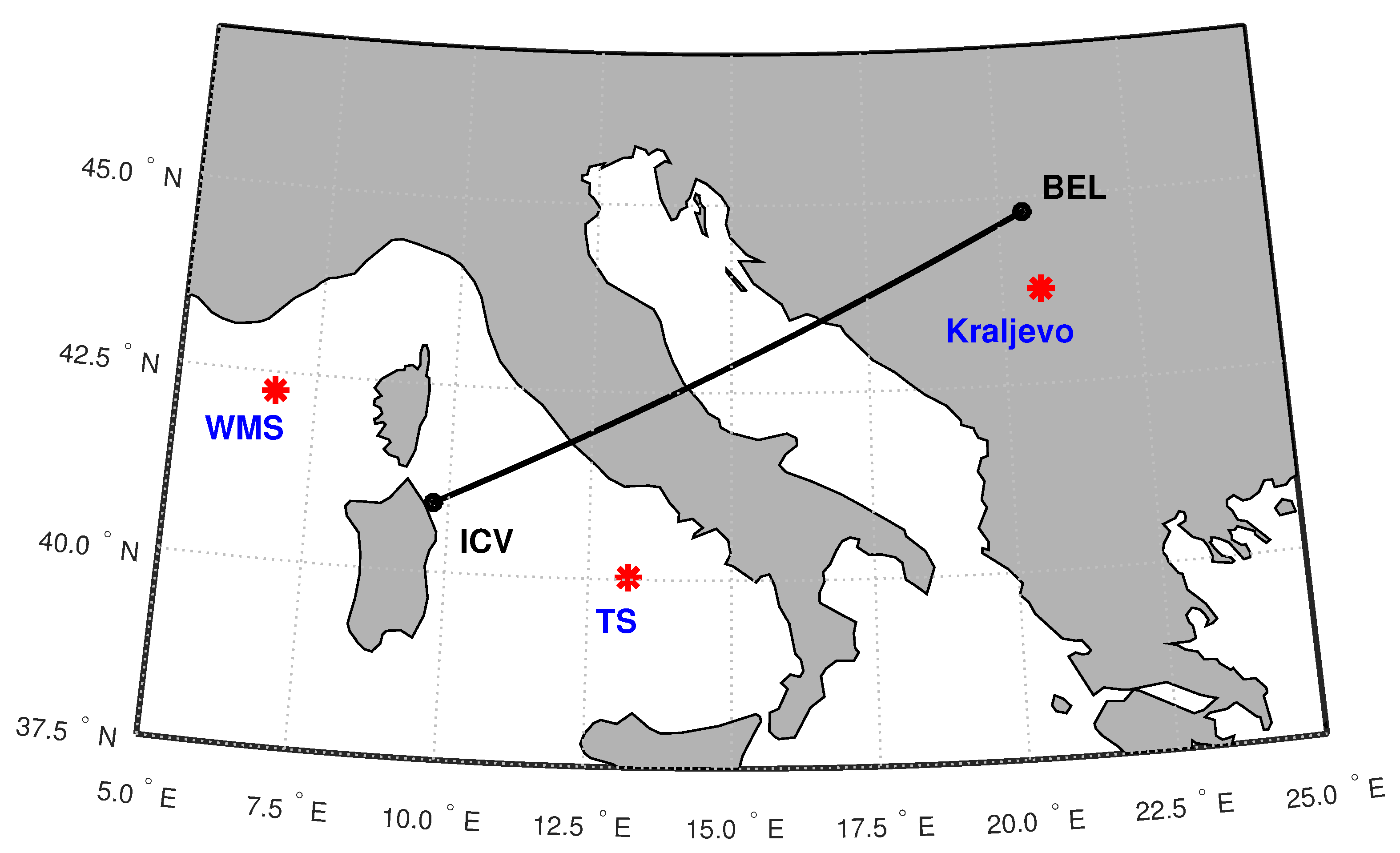
In this study we analyse phase of the ICV signal emitted by a transmitter located in Isola di Tavolara, Italy (40.92 N, 9.73 E) and received in Belgrade, Serbia (44.8 N, 20.4 E) in time periods around four EQs, considered in [33] and connected to the short-term noise amplitude reduction. Two of these events occurred near Kraljevo, Serbia, one in the Tyrrhenian Sea (TS) and one in the Western Mediterranean Sea (WMS) (their epicentres are shown in map given in Figure 1). As it can be seen in Table 1, their magnitudes were greater than 5 for two events (the first one near Kraljevo, and in the Tyrrhenian Sea) while other two had magnitude larger than 4. These magnitudes are larger than those related to other EQs considered in [33].
During the considered four time intervals, additional weaker EQs also occurred near the considered signal propagation path. After the most intensive EQ (Kraljevo, 3/11/2010) 31 additional EQs occurred before 8 UT. 27 of these events were in Serbia, 3 in Italy and 1 in Bosnia and Herzegovina. Their magnitudes were lower than 3 except in one case when it was 3.3. Because of this large number we only give common information of their occurrences in Table 1. Processes in the lithosphere below the monitored ionospheric area were not so intensive during the other three time intervals. For this reason all additional EQ events are indicated in Table 1.
In this analysis, we process the 0.1-s resolution datasets. This procedure consists of three parts: (1) phase unwrapping, (2) determination of the unwrapped phase noise, and (3) application of Fast Fourier Transform (FFT) to the unwrapped phase in order to examine excitations and attenuations of the acoustic and gravity waves.
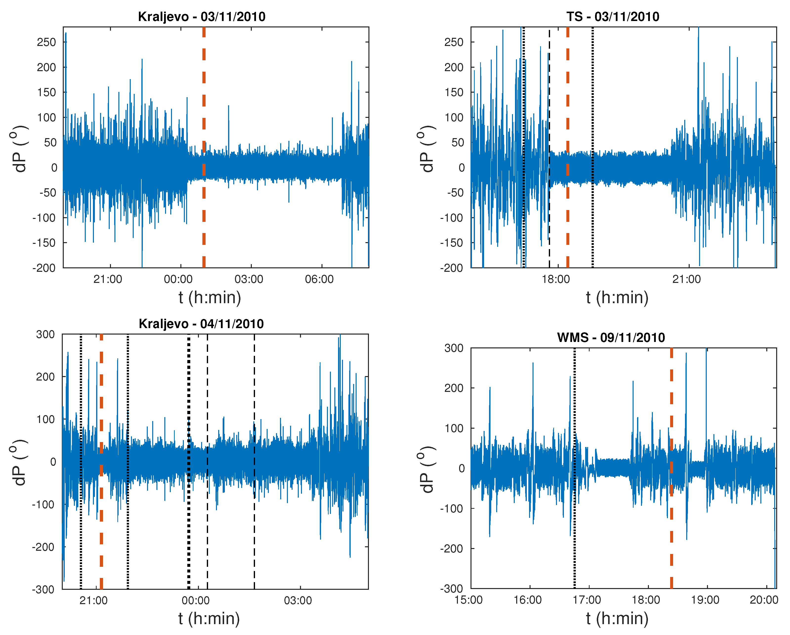
- Phase unwrapping. The recorded signal phase represents the deviation of the signal phase with respect to the phase generated at the receiver. Because of that it has a component of constant slope. However, this component does not affect the presented analysis, and for this reason we did not remove it. On the other side, all recorded values are given within a principal phase interval and for further analysis it is necessary to unwrap it. The obtained time evolutions of the unwrapped phase P are shown in Figure 2 where the vertical lines indicate times of EQ occurrences. Red lines represent the main EQ considered in corresponding time periods while the additional events listed in Table 1 are coloured in black. To visualize the magnitudes of these additional events, we divided them in three categories: 1. magnitude below 2.5, 2. magnitudes from 2.5 to 3, and 3. magnitudes from 3 to 4. These categories are represented by thin dotted, thin dashed and tick dotted black lines, respectively.
- Determination of the phase noise. To obtain the noise of the unwrapped phase P we calculate its deviation from the basic phase at time t. Here, is obtained in a procedure described in [33] as the mean value of unwrapped phase in the defined time bins around time t. Finally, noise of P is determined as the maximum of after elimination of the largest p percent of its values. To find this value, we first sorted the values of into an ascending array of N members, and determined the value of the phase noise as the value of the term that is in this array:In this study we use like in [33].
- Acoustic and gravity waves—excitations and attenuations. Research of the acoustic and gravity waves in this paper is based on processing of the VLF signal phase. We analyse their excitations and attenuations in periods around the considered EQs using the procedure given in [33]. It is based on the application of the Fast Fourier Transform (FFT) on fixed window time intervals (WTI) within the considered time periods. Keeping in mind that WTI affects the maximum of observable wave period and precision in the analysis of the observed variations we choose three WTIs of 20 min, 1 h and 3 h.The goal of this procedure is to analyse the recorded phase in frequency domain and connect the wave-periods for which important changes are recorded to the acoustic and gravity waves. The acoustic cut-off and the Brunt-Väisälä wave-periods representing minimal and maximal periods for the acoustic and gravity waves, respectively, are determined from the expressions:where is the standard ratio of specific heats and m/s is gravitational acceleration. The adiabatic sound speed squared is obtained for the gass temperature K (estimated from the International Reference Ionosphere (IRI) model [41] and assumed average mass of atoms kg. The Boltzmann constant is J/K. Details of this procedure can be found in, for example, [42,43].As it is obtained in [33] waves with periods , s and s, represents acoustic and gravity modes, respectively.
Here we point out that during the considered time periods there are not recorded other events which can influence the signal phase. Detailed analysis, described in [33], indicated that influences of receiver, transmitter, meteorological and geomagnetic conditions, which are suggested as the most important non-ionospheric sources of the VLF signal variations [44], can be ignored.
3. Results and Discussions
Results of determination of the phase noise and periods of the excited and attenuated acoustic and gravity waves are presented in Section 3.1 and Section 3.2, respectively.
3.1. Signal Phase Noise
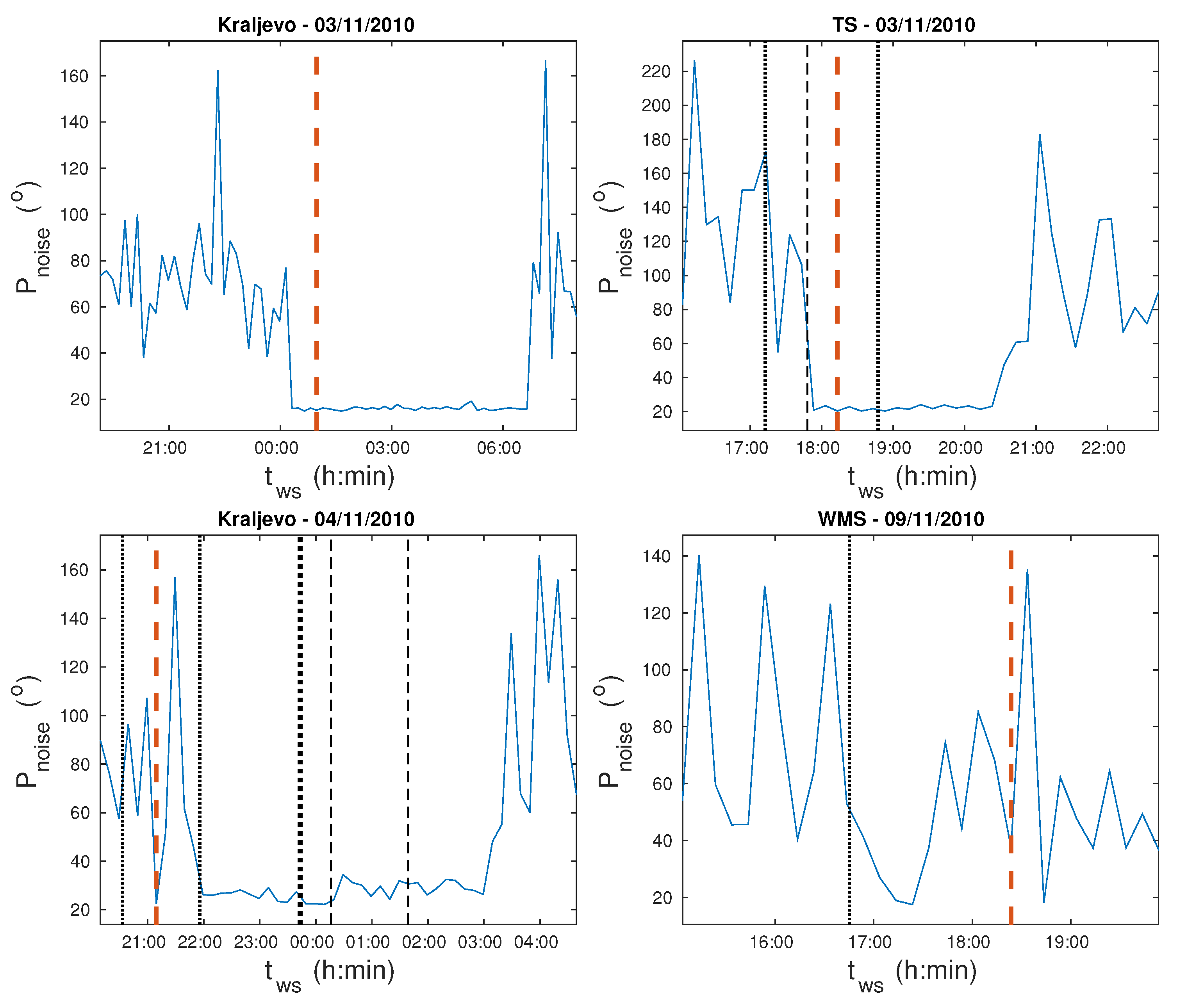
Time evolutions of deviation of the wrapped phase from its basic values dP and the phase noise obtained by the proposed methodology are shown in Figure 3 and Figure 4, respectively. As one can see, reduction of the phase noise is recorded for all four main EQ events and it is clearly visible in the first two cases whose magnitudes are greater than 5.
It is worth noting that after the first EQ event near Kraljevo which occurred on 3 November 2010, additional 31 EQs occurred in areas near the considered signal propagation path. Twenty nine of them occurred when the phase noise reduction is clearly visible, while two events of weak intensities (magnitudes of 2.1 and 2.2) occurred after increasing of the phase noise. The most intensive additional EQ had magnitude of 3.3. However, despite the large number of accompanying earthquakes, no significant variations were observed either in dP or in . The absence of these variations is also noticeable in the second case (EQ in Tyrrhenian Sea of magnitude 5.1) when three more earthquakes (magnitudes of 2, 2.1 and 2.5) were recorded within about 1.5 h.
In the cases of the other two EQs which magnitudes were between 4 and 5, analysis of dP and time evolutions is not so simple like in the first two considered time intervals. Namely, although the reductions in phase noise are recorded before and after these events, they are not related each other. In the case of the EQ which occurred near Kraljevo on 4 November 2010 significant reduction in is recorded several minutes before the EQ and lasts about 20 min. This phase reduction is followed by the short-term increase in and additional significant decrease which yield to the second reduction lasting about 5 h. During the second reduction four additional EQs are recorded. The first one occurred in North Italy while the other three near Kraljevo (like the main one) with magnitudes of 3.3, 2.8 and 2.5. As one can see in the bottom left panels of Figure 3 and Figure 4, although the small increase in noise is recorded after the second additional EQ near Kraljevo, significant reduction which can be related with EQ events observed within a time window of about 3 h and includes the time of the last EQ.
Reduction of the phase noise begins about 1 h before the EQ in the Western Mediterranean Sea but it is also possible relate it with the EQ occurred in Central Italy just before the decrease in dP . This reduction is followed by noise increase which begins more than a half of hour before the EQ and lasts about 1 h before the reduction is recorded again. This event is interesting because position of the EQ epicentre is, contrary to the other events, northern than the signal propagation path. The possible recorded time shift of the reduction time opens a question of influence of position of the EQ epicentre with respect to the signal propagation path. This task requires a specific statistical analysis and it will be in focus of our forthcoming research.
By comparison with noise amplitude reduction analysed in [33] we can conclude that the characteristics of phase reduction are the same for the first two cases: they last for several hours, begin before and end after an EQ event, and there are not observed changes that could be related to other earthquakes of lower intensity. In the third and fourth cases phase noise reductions are also recorded, but they are shortly interrupted by the noise amplifications. Also, it cannot be claimed that the strongest earthquake in the observed period masks the potential relationship between phase noise reduction and weaker EQs.
3.2. Acoustic and Gravity Waves
In the second part of this study we analyse signal phase in frequency domain. We apply FFT to the recorded data to research possible excitations and attenuations of the acoustic and gravity waves that can be considered as ionospheric disturbances connected to earthquakes.
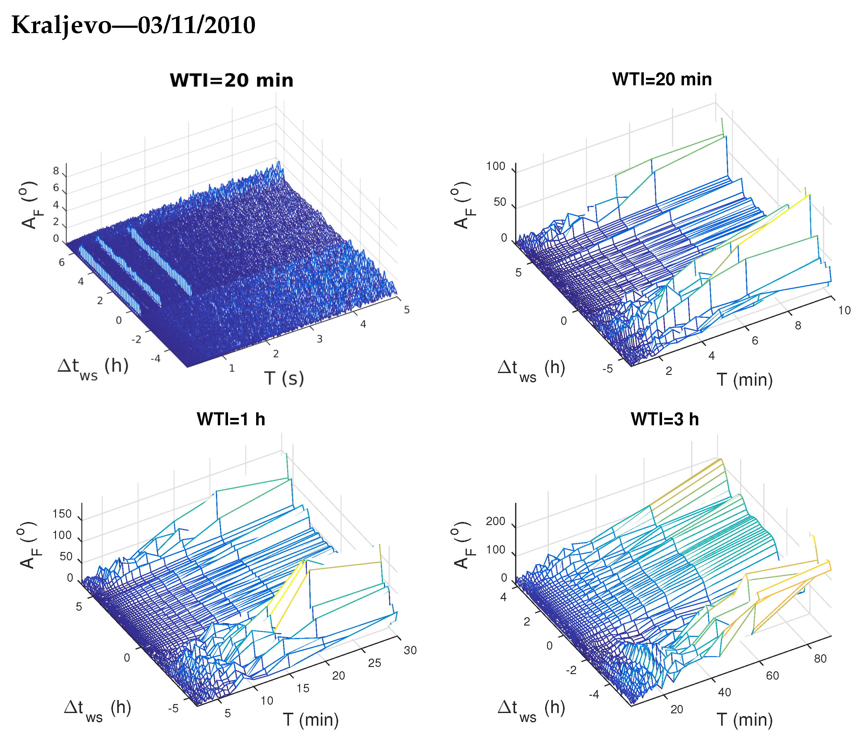
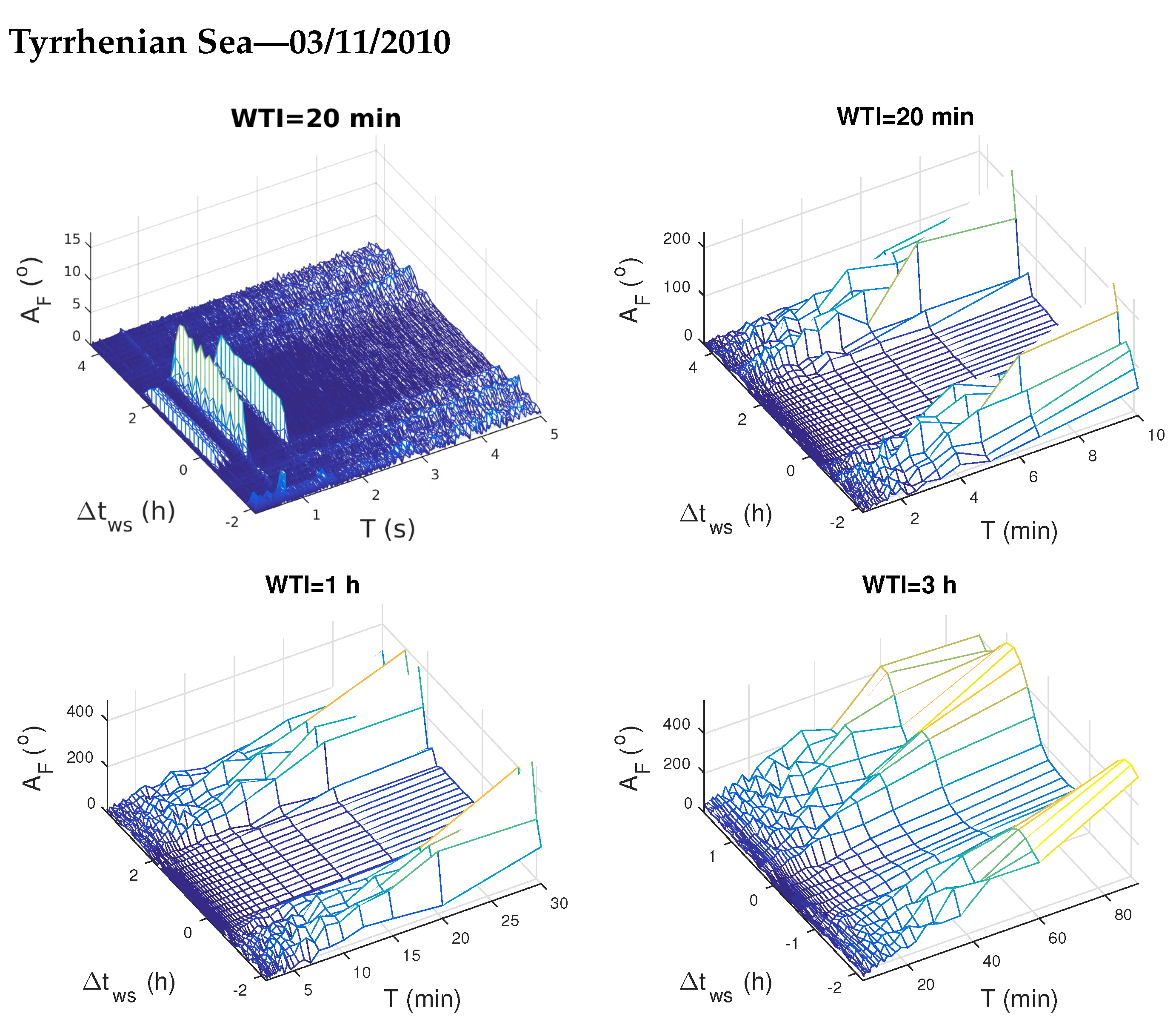
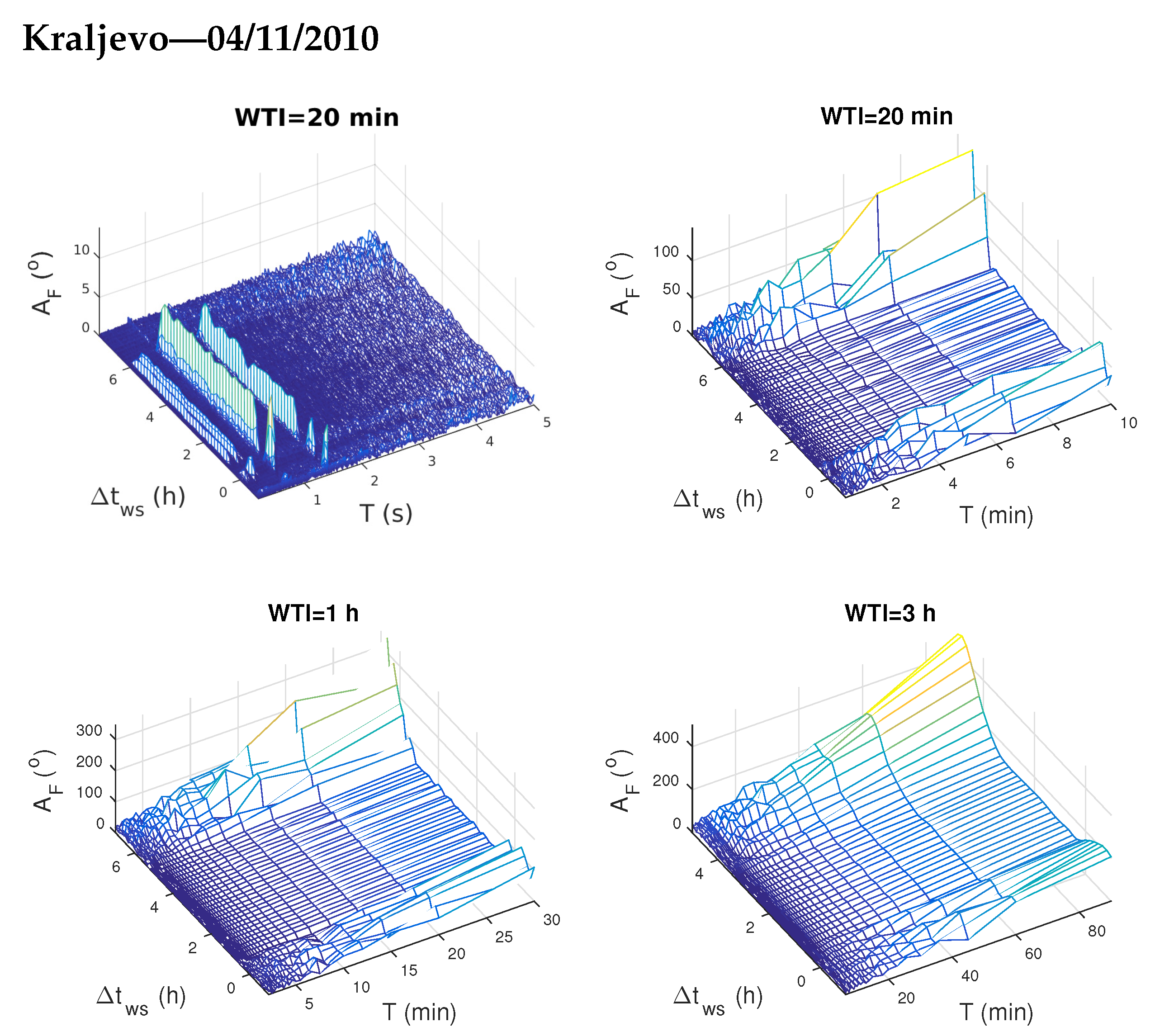
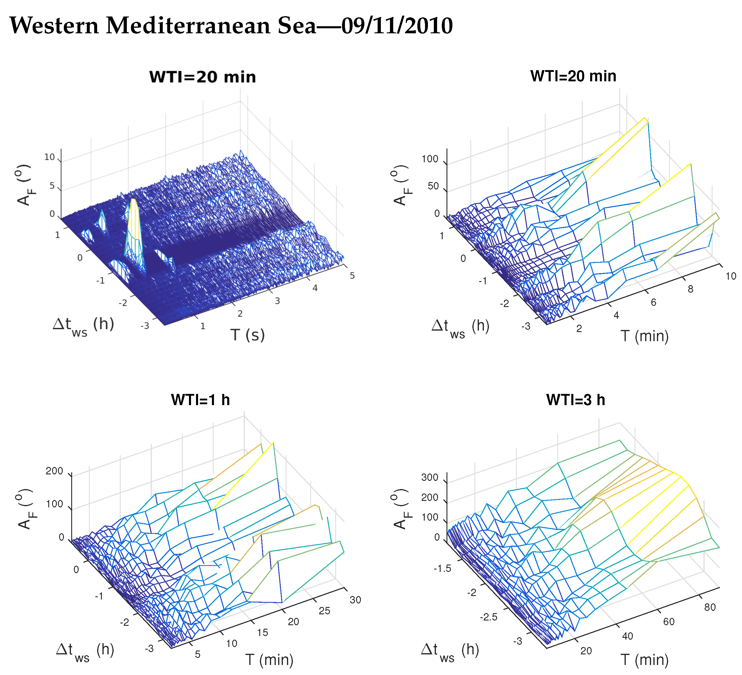
To better visualize periods of the excited/attenuated waves we apply the same procedures like in [33]: (1) we consider three WTI of 20 min, 1 h and 3 h and, (2) in order to better present changes for smaller and greater wave periods T, the obtained values for all WTIs are considered for smaller and greater wave period domains separately. In this study we showed lower periods T for the first WTI, and greater periods for all the three WTIs. The results of the analyses for the considered four time periods are shown in Figure 5, Figure 6, Figure 7 and Figure 8.
Similarly to the analysis of the noise amplitude shown in [33], excitations are recorded in periods when phase noise is reduced at several values of T which are smaller than 1.5 s:
- Kraljevo—03/11/2010: 0.2 s, 0.23 s, 0.47 s (weak increase of the Fourier amplitude), 0.7 s and 1.4 s.
- Tyrrhenian Sea—03/11/2010: 0.23 s, 0.35 s, 0.47 s, 0.7 s and 1.4 s.
- Kraljevo—04/11/2010: 0.23 s, 0.35 s, 0.7 s and 1.4 s;
- Western Mediterranean Sea—09/11/2010: 0.23 s, 0.35 s, 0.47 s (during the first time period when noise reduction is recorded), 0.7 s and 1.4 s.
As one can see, the common periods are 0.23 s, 0.35 s, and 1.4 s while waves at period of 0.47 s are exited in three cases whereby these excitations are weak in the first case, while in the forth case they are recorded only for one of two periods of phase noise reduction. Excited waves at 0.2 s are recorded only for the first considered EQ event. Because the obtained values are lower than calculated maximum period of the acoustic waves () we can conclude that acoustic waves are excited in periods when noise reduction occurs.
Although the previous results related to the noise reductions and excitations of the acoustic waves are very similar as those shown in analysis of the amplitude, there is a difference in wave attenuation. Namely, the Fourier amplitude for several discrete values before the reduction time are reported in [33]. In this study, these peaks are not recorded. In addition, in all four considered periods attenuations are clearly visible at all periods T (except those values for which excitation is recorded) for phase while these attenuations are much less pronounced in the case of the amplitude for time period around Kraljevo EQ on 3 November 2010. Recent results obtained for the Kumamoto M7.2 earthquake on 15 April 2016 in Japan [45] are in close correlation with our results, so we can suppose that registered oscillations are the acoustic gravity waves of the same origin as is described in this paper. A similar correlation of our results can be also found in their comparison with data presented in analysis of the M7.8 earthquake with the epicenter in Nepal on 25 April 2015 [46].
4. Conclusions
In this paper we analysed the VLF signal phase in time periods around four earthquakes which magnitude were greater than 4. The goal of this study was to extend analyses of reductions of the noise amplitude of VLF signals, excitations and attenuations of the acoustic and gravity waves presented in [33] to the corresponding analyses of the phase of the VLF signal. We analysed data recorded by the receiver located in Belgrade, Serbia for VLF signal emitted by the ICV transmitter in Italy.
The obtained results of this study can be summarised as follows:
- In the cases of EQs with magnitudes greater than 5, a multi-hour noise reductions was observed. As in the case of the amplitude, they begin before the earthquake. In these cases, no changes that could be related to other earthquakes of lower intensity were observed.
- In the cases of EQs with magnitudes between 4 and 5, phase noise reductions are also recorded, but they are shortly interrupted by the noise amplifications. Specific reductions are potentially related to different EQs, i.e., it cannot be claimed that the strongest earthquake in the observed period masks the potential relationship between phase noise reduction and weaker EQs.
- Because the recorded phase reductions are very similar like those in the case of the amplitude the choice of the signal characteristic which can be used in the corresponding studies depends only on the quality of the recorded data and do not affect the results of study.
- Excitations of the acoustic waves are recorded for all four periods. The obtained wave-periods are below 1.5 s which is in agreement with results obtained in analysis of the amplitude.
- Attenuations of the acoustic and gravity waves are recorded continuously with wave-period except for those T corresponding to wave excitations. This result does not agree with those obtained when analysing amplitude variations where attenuations are primarily recorded for discrete values of wave periods, while similar continuous attenuations are much less pronounced.
Author Contributions
Conceptualization, methodology, investigation, resources, formal analysis, writing—original draft, preparation, visualization, A.N.; software, data curation, A.N. and S.T.M.; validation, P.F.B., S.P., L.Č.P. and M.R.; writing—review and editing, all authors. All authors have read and agreed to the published version of the manuscript.
Funding
The authors acknowledge funding provided by the Institute of Physics Belgrade, the Astronomical Observatory (the contract 451-03-68/2020-14/200002) through the grants by the Ministry of Education, Science, and Technological Development of the Republic of Serbia.
Institutional Review Board Statement
Not applicable.
Informed Consent Statement
Not applicable.
Data Availability Statement
Publicly available datasets were analysed in this study. This data can be found here: http://www.emsc-csem.org/Earthquake/ (accessed on 28 February 2021); https://ccmc.gsfc.nasa.gov/modelweb/models/iri2012_vitmo.php (accessed on 29 February 2021). The VLF data used for analysis is available from the corresponding author.
Acknowledgments
This research was supported by COST Actions CA18109 and CA15211.
Conflicts of Interest
The authors declare no conflict of interest.
Sample Availability
The VLF data used for analysis is available from the corresponding author.
References
- Bilitza, D. IRI the International Standard for the Ionosphere. Adv. Radio Sci. 2018, 16, 1–11. [Google Scholar] [CrossRef] [Green Version]
- Nina, A.; Nico, G.; Mitrović, S.T.; Čadež, V.M.; Milošević, I.R.; Radovanović, M.; Popović, L.Č. Quiet Ionospheric D-Region (QIonDR) Model Based on VLF/LF Observations. Remote Sens. 2021, 13, 483. [Google Scholar] [CrossRef]
- Nina, A.; Nico, G.; Odalović, O.; Čadež, V.M.; Drakul, M.T.; Radovanović, M.; Popović, L.Č. GNSS and SAR Signal Delay in Perturbed Ionospheric D-Region During Solar X-Ray Flares. IEEE Geosci. Remote Sens. Lett. 2020, 17, 1198–1202. [Google Scholar] [CrossRef]
- Pulinets, S.; Boyarchuk, K. Ionospheric Precursor of Earthquakes; Springer: Berlin/Heidelberg, Germany, 2004. [Google Scholar] [CrossRef]
- Rozhnoi, A.; Solovieva, M.; Molchanov, O.; Hayakawa, M. Middle latitude LF (40 kHz) phase variations associated with earthquakes for quiet and disturbed geomagnetic conditions. Phys. Chem. Earth 2004, 29, 589–598. [Google Scholar] [CrossRef]
- Hayakawa, M. VLF/LF Radio Sounding of Ionospheric Perturbations Associated with Earthquakes. Sensors 2007, 7, 1141–1158. [Google Scholar] [CrossRef] [Green Version]
- Liu, Y.; Jin, S. Ionospheric Rayleigh Wave Disturbances Following the 2018 Alaska Earthquake from GPS Observations. Remote Sens. 2019, 11, 901. [Google Scholar] [CrossRef] [Green Version]
- Zhong, M.; Shan, X.; Zhang, X.; Qu, C.; Guo, X.; Jiao, Z. Thermal Infrared and Ionospheric Anomalies of the 2017 Mw6.5 Jiuzhaigou Earthquake. Remote Sens. 2020, 12, 2843. [Google Scholar] [CrossRef]
- Biagi, P.F.; Piccolo, R.; Ermini, A.; Martellucci, S.; Bellecci, C.; Hayakawa, M.; Kingsley, S.P. Disturbances in LF radio-signals as seismic precursors. Ann. Geophys. 2001, 44, 5–6. [Google Scholar] [CrossRef]
- Hayakawa, M. Probing the lower ionospheric perturbations associated with earthquakes by means of subionospheric VLF/LF propagation. Earthq. Sci. 2011, 24, 609–637. [Google Scholar] [CrossRef] [Green Version]
- Nina, A.; Radovanović, M.; Milovanović, B.; Kovačević, A.; Bajčetić, J.; Popović, L.Č. Low ionospheric reactions on tropical depressions prior hurricanes. Adv. Space Res. 2017, 60, 1866–1877. [Google Scholar] [CrossRef] [Green Version]
- Rozhnoi, A.; Shalimov, S.; Solovieva, M.; Levin, B.; Hayakawa, M.; Walker, S. Tsunami-induced phase and amplitude perturbations of subionospheric VLF signals. J. Geophys. Res. Space 2012, 117, 9313. [Google Scholar] [CrossRef]
- Molchanov, O.; Hayakawa, M.; Oudoh, T.; Kawai, E. Precursory effects in the subionospheric VLF signals for the Kobe earthquake. Phys. Earth Planet. Inter. 1998, 105, 239–248. [Google Scholar] [CrossRef]
- Žigman, V.; Grubor, D.; Šulić, D. D-region electron density evaluated from VLF amplitude time delay during X-ray solar flares. J. Atmos. Sol. Terr. Phys. 2007, 69, 775–792. [Google Scholar] [CrossRef]
- Srećković, V.; Šulić, D.; Vujičić, V.; Jevremović, D.; Vyklyuk, Y. The effects of solar activity: Electrons in the terrestrial lower ionosphere. J. Geogr. Inst. Cvijic 2017, 67, 221–233. [Google Scholar] [CrossRef]
- Raulin, J.P.; Trottet, G.; Kretzschmar, M.; Macotela, E.L.; Pacini, A.; Bertoni, F.C.P.; Dammasch, I.E. Response of the low ionosphere to X-ray and Lyman-α solar flare emissions. J. Geophys. Res. Space 2013, 118, 570–575. [Google Scholar] [CrossRef] [Green Version]
- Basak, T.; Chakrabarti, S.K. Effective recombination coefficient and solar zenith angle effects on low-latitude D-region ionosphere evaluated from VLF signal amplitude and its time delay during X-ray solar flares. Astrophys. Space Sci. 2013, 348, 315–326. [Google Scholar] [CrossRef] [Green Version]
- Chakraborty, S.; Basak, T. Numerical analysis of electron density and response time delay during solar flares in mid-latitudinal lower ionosphere. Astrophys. Space Sci. 2020, 365, 1–9. [Google Scholar] [CrossRef]
- Kumar, S.; NaitAmor, S.; Chanrion, O.; Neubert, T. Perturbations to the lower ionosphere by tropical cyclone Evan in the South Pacific Region. J. Geophys. Res. Space 2017, 122, 8720–8732. [Google Scholar] [CrossRef]
- Rozhnoi, A.; Solovieva, M.; Levin, B.; Hayakawa, M.; Fedun, V. Meteorological effects in the lower ionosphere as based on VLF/LF signal observations. Nat. Hazards Earth Syst. Sci. 2014, 14, 2671–2679. [Google Scholar] [CrossRef] [Green Version]
- Singh, R.; Veenadhari, B.; Maurya, A.K.; Cohen, M.B.; Kumar, S.; Selvakumaran, R.; Pant, P.; Singh, A.K.; Inan, U.S. D-region ionosphere response to the total solar eclipse of 22 July 2009 deduced from ELF-VLF tweek observations in the Indian sector. J. Geophys. Res. Space 2011, 116, 10301. [Google Scholar] [CrossRef] [Green Version]
- Ilić, L.; Kuzmanoski, M.; Kolarž, P.; Nina, A.; Srećković, V.; Mijić, Z.; Bajčetić, J.; Andrić, M. Changes of atmospheric properties over Belgrade, observed using remote sensing and in situ methods during the partial solar eclipse of 20 March 2015. J. Atmos. Sol. Terr. Phys. 2018, 171, 250–259. [Google Scholar] [CrossRef]
- Jin, S.; Occhipinti, G.; Jin, R. GNSS ionospheric seismology: Recent observation evidences and characteristics. Earth Sci. Rev. 2015, 147, 54–64. [Google Scholar] [CrossRef]
- Manta, F.; Occhipinti, G.; Feng, L.; Hill, E.M. Rapid identification of tsunamigenic earthquakes using GNSS ionospheric sounding. Sci. Rep. 2020, 10, 1–10. [Google Scholar] [CrossRef]
- Korepanov, V.; Hayakawa, M.; Yampolski, Y.; Lizunov, G. AGW as a seismo-ionospheric coupling responsible agent. Phys. Chem. Earth 2009, 34, 485–495. [Google Scholar] [CrossRef]
- Mareev, E.A. Mosaic source of internal gravity waves associated with seismic activity. Seism. Electromagn. Lithosphere Atmos. Ionos. 2002, 335–343. [Google Scholar] [CrossRef]
- Molchanov, O.; Fedorov, E.; Schekotov, A.; Gordeev, E.; Chebrov, V.; Surkov, V.; Rozhnoi, A.; Andreevsky, S.; Iudin, D.; Yunga, S.; et al. Lithosphere-atmosphere-ionosphere coupling as governing mechanism for preseismic short-term events in atmosphere and ionosphere. Nat. Haz. Earth Syst. Sci. 2004, 4, 757–767. [Google Scholar] [CrossRef] [Green Version]
- Nina, A.; Čadež, V.M. Detection of acoustic-gravity waves in lower ionosphere by VLF radio waves. Geophys. Res. Lett. 2013, 40, 4803–4807. [Google Scholar] [CrossRef] [Green Version]
- Kumar, S.; Kumar, A.; Menk, F.; Maurya, A.K.; Singh, R.; Veenadhari, B. Response of the low-latitude D region ionosphere to extreme space weather event of 14–16 December 2006. J. Geophys. Res. Space 2015, 120, 788–799. [Google Scholar] [CrossRef] [Green Version]
- Maurya, A.K.; Venkatesham, K.; Kumar, S.; Singh, R.; Tiwari, P.; Singh, A.K. Effects of St. Patrick’s Day Geomagnetic Storm of March 2015 and of June 2015 on Low-Equatorial D Region Ionosphere. J. Geophys. Res. Space 2018, 123, 6836–6850. [Google Scholar] [CrossRef]
- NaitAmor, S.; Cohen, M.B.; Kumar, S.; Chanrion, O.; Neubert, T. VLF Signal Anomalies During Cyclone Activity in the Atlantic Ocean. Geophys. Res. Lett. 2018, 45, 10,185–10,192. [Google Scholar] [CrossRef] [Green Version]
- Kumar, S.; Kumar, A.; Maurya, A.K.; Singh, R. Changes in the D region associated with three recent solar eclipses in the South Pacific region. J. Geophys. Res. Space 2016, 121, 5930–5943. [Google Scholar] [CrossRef] [Green Version]
- Nina, A.; Pulinets, S.; Biagi, P.; Nico, G.; Mitrović, S.; Radovanović, M.; Popović, Č.L. Variation in natural short-period ionospheric noise, and acoustic and gravity waves revealed by the amplitude analysis of a VLF radio signal on the occasion of the Kraljevo earthquake (Mw = 5.4). Sci. Total Environ. 2020, 710, 136406. [Google Scholar] [CrossRef]
- Maurya, A.K.; Phanikumar, D.V.; Singh, R.; Kumar, S.; Veenadhari, B.; Kwak, Y.S.; Kumar, A.; Singh, A.K.; Niranjan Kumar, K. Low-mid latitude D region ionospheric perturbations associated with 22 July 2009 total solar eclipse: Wave-like signatures inferred from VLF observations. J. Geophys. Res. 2014, 119, 8512–8523. [Google Scholar] [CrossRef] [Green Version]
- Yamauchi, T.; Maekawa, S.; Horie, T.; Hayakawa, M.; Soloviev, O. Subionospheric VLF/LF monitoring of ionospheric perturbations for the 2004 Mid-Niigata earthquake and their structure and dynamics. J. Atmos. Sol. Terr. Phys. 2007, 69, 793–802. [Google Scholar] [CrossRef]
- Maekawa, S.; Horie, T.; Yamauchi, T.; Sawaya, T.; Ishikawa, M.; Hayakawa, M.; Sasaki, H. A statistical study on the effect of earthquakes on the ionosphere, based on the subionospheric LF propagation data in Japan. Ann. Geophys. 2006, 24, 2219–2225. [Google Scholar] [CrossRef]
- Maurya, A.K.; Venkatesham, K.; Tiwari, P.; Vijaykumar, K.; Singh, R.; Singh, A.K.; Ramesh, D.S. The 25 April 2015 Nepal Earthquake: Investigation of precursor in VLF subionospheric signal. J. Geophys. Res. Space 2016, 121, 10,403–10,416. [Google Scholar] [CrossRef] [Green Version]
- Zhao, S.; Shen, X.; Liao, L.; Zhima, Z.; Zhou, C.; Wang, Z.; Cui, J.; Lu, H. Investigation of Precursors in VLF Subionospheric Signals Related to Strong Earthquakes (M > 7) in Western China and Possible Explanations. Remote Sens. 2020, 12, 3563. [Google Scholar] [CrossRef]
- Biagi, P.; Castellana, L.; Maggipinto, T.; Maggipinto, G.; Minafra, A.; Ermini, A.; Molchanov, O.; Rozhnoi, A.; Solovieva, M.; Hayakawa, M. Anomalies in VLF radio signals related to the seismicity during November–December 2004: A comparison of ground and satellite results. Phys. Chem. Earth Parts A/B/C 2009, 34, 456–463. [Google Scholar] [CrossRef]
- Knezevic Antonijevic, S.; Arroucau, P.; Vlahovic, G. Seismotectonic Model of the Kraljevo 3 November 2010 Mw 5.4 Earthquake Sequence. Seismol. Res. Lett. 2013, 84, 600–610. [Google Scholar] [CrossRef]
- International Reference Ionosphere—IRI-2012. Available online: https://ccmc.gsfc.nasa.gov/modelweb/models/iri2012_vitmo.php (accessed on 28 February 2021).
- Yeh, K.C.; Liu, C.H. Theory of Ionospheric Waves; Academic Press: New York, NY, USA, 1972. [Google Scholar]
- Goedbloed, H.; Poedts, S. Principles of Magnetohydrodynamics: With Applications to Laboratory and Astrophysical Plasmas; Cambridge University Press: Cambridge, UK, 2004. [Google Scholar]
- Biagi, P.F.; Maggipinto, T.; Righetti, F.; Loiacono, D.; Schiavulli, L.; Ligonzo, T.; Ermini, A.; Moldovan, I.A.; Moldovan, A.S.; Buyuksarac, A.; et al. The European VLF/LF radio network to search for earthquake precursors: Setting up and natural/man-made disturbances. Nat. Hazards Earth Syst. Sci. 2011, 11, 333–341. [Google Scholar] [CrossRef]
- Yang, S.S.; Asano, T.; Hayakawa, M. Abnormal Gravity Wave Activity in the Stratosphere Prior to the 2016 Kumamoto Earthquakes. J. Geophys. Res. Space 2019, 124, 1410–1425. [Google Scholar] [CrossRef]
- Chum, J.; Liu, J.-Y.; Laštovička, J.; Fišer, J.; Mošna, Z.; Sun, Y.-Y. Ionospheric signatures of the 25 April 2015 Nepal earthquake and the relative role of compression and advection for Doppler sounding of infrasound in the ionosphere. Earth Planets Space 2019, 68, 24. [Google Scholar] [CrossRef] [Green Version]
Figure 1.
Propagation paths of the VLF signals recorded by the Belgrade receiver station (BEL) in Serbia and emitted by the transmitters ICV in Italy. Locations of the main considered EQs are shown as stars. One EQ occurred in the Tyrrhenian Sea (TS) and Western Mediterranean Sea (WMS), while two EQs were near Kraljevo (their epicentres are shown by the same star).

Figure 2.
Time evolutions of the unwrapped phase P for the considered periods. Red lines represent the main EQ considered in corresponding time periods. The additional events listed in Table 1 are coloured in black. Times of the additional considered EQ events with magnitude below 2.5, from 2.5 to 3, and from 3 to 4 are represented by thin dotted, thin dashed and tick dotted black lines, respectively.

Figure 3.
The same as in Figure 2 but for phase deviation .
Figure 3.
The same as in Figure 2 but for phase deviation .

Figure 4.
The same as in Figure 2 but for the phase noise .
Figure 4.
The same as in Figure 2 but for the phase noise .

Figure 5.
Fourier amplitude of waves with period T obtained by applying FFT to the ICV signal phase recorded in time around EQ occurred near Kraljevo on 3 November 2010 with window time intervals (WTI) of 20 min (upper panels), 1 h (bottom left panel), and 3 h (bottom right panel) which begin with a shift with respect to the EQ time.

Figure 6.
Fourier amplitude of waves with period T obtained by applying FFT to the ICV signal phase recorded in time around EQ occurred in the Tyrrhenian Sea on 3 November 2010 with window time intervals (WTI) of 20 min (upper panels), 1 h (bottom left panel), and 3 h (bottom right panel) which begin with a shift with respect to the EQ time.

Figure 7.
Fourier amplitude of waves with period T obtained by applying FFT to the ICV signal phase recorded in time around EQ occurred near Kraljevo on 4 November 2010 with window time intervals (WTI) of 20 min (upper panels), 1 h (bottom left panel), and 3 h (bottom right panel) which begin with a shift with respect to the EQ time.

Figure 8.
Fourier amplitude of waves with period T obtained by applying FFT to the ICV signal phase recorded in time around EQ occurred in the Western Mediterranean Sea on 9 November 2010 with window time intervals (WTI) of 20 min (upper panels), 1 h (bottom left panel), and 3 h (bottom right panel) which begin with a shift with respect to the EQ time.


Table 1.
List of the main earthquakes considered in this study. EQ date, time t, epicentre locations (latitude (LAT) and longitude (LON)) and magnitudes (M) are given in http://www.emsc-csem.org/Earthquake/(accessed on 25 February 2021). The variable d denotes the distance between the EQ epicentres and signal propagation path.
| No. | Date | t (UTC) | LAT () | LON () | d (km) | M | Location |
|---|---|---|---|---|---|---|---|
| Kraljevo—03/11/2010 | |||||||
| 1 | 2010/11/03 | 00:56:54 | 43.74 | 20.69 | 126.0 | 5.4 | Serbia (near Kraljevo) |
| 31 EQs until 8 UT—31 in Serbia, 3 in Italy and 1 in Bosnia and Herzegovina | |||||||
| Tyrrhenian Sea (TS)—03/11/2010 | |||||||
| 2 | 2010-11-03 | 17:12:30 | 42.4 | 13.35 | 11.4 | 2 | Central Italy |
| 2010-11-03 | 17:48:04 | 43.75 | 20.7 | 120.7 | 2.5 | Serbia (near Kraljevo) | |
| 2010/11/03 | 18:13:10 | 40.03 | 13.2 | 219.1 | 5.1 | TS | |
| 2010-11-03 | 18:47:23 | 43.73 | 20.67 | 121.7 | 2.1 | Serbia (near Kraljevo) | |
| Kraljevo—04/11/2010 | |||||||
| 1 | 2010-11-04 | 20:33:01 | 43.75 | 20.7 | 120.7 | 1.9 | Serbia (near Kraljevo) |
| 2010/11/04 | 21:09:05 | 43.78 | 20.62 | 114.9 | 4.4 | Serbia (near Kraljevo) | |
| 2010-11-04 | 21:55:40 | 45.81 | 7.55 | 562.9 | 1.2 | Northern Italy | |
| 2010-11-04 | 23:43:05 | 43.78 | 20.62 | 114.9 | 3.3 | Serbia (near Kraljevo) | |
| 2010-11-05 | 00:16:14 | 43.74 | 20.64 | 119.6 | 2.8 | Serbia (near Kraljevo) | |
| 2010-11-05 | 01:38:48 | 43.76 | 20.69 | 119.4 | 2.5 | Serbia (near Kraljevo) | |
| Western Mediterranean Sea (WMS)—03/11/2010 | |||||||
| 4 | 2010-11-09 | 16:45:13 | 43.59 | 12.36 | 165.9 | 2.3 | Central Italy |
| 2010-11-09 | 18:23:36 | 42.25 | 6.77 | 287.7 | 4.3 | WMS | |
Publisher’s Note: MDPI stays neutral with regard to jurisdictional claims in published maps and institutional affiliations. |
© 2021 by the authors. Licensee MDPI, Basel, Switzerland. This article is an open access article distributed under the terms and conditions of the Creative Commons Attribution (CC BY) license (https://creativecommons.org/licenses/by/4.0/).
Share and Cite
MDPI and ACS Style
Nina, A.; Biagi, P.F.; Mitrović, S.T.; Pulinets, S.; Nico, G.; Radovanović, M.; Popović, L.Č. Reduction of the VLF Signal Phase Noise Before Earthquakes. Atmosphere 2021, 12, 444. https://doi.org/10.3390/atmos12040444
AMA Style
Nina A, Biagi PF, Mitrović ST, Pulinets S, Nico G, Radovanović M, Popović LČ. Reduction of the VLF Signal Phase Noise Before Earthquakes. Atmosphere. 2021; 12(4):444. https://doi.org/10.3390/atmos12040444
Chicago/Turabian StyleNina, Aleksandra, Pier Francesco Biagi, Srđan T. Mitrović, Sergey Pulinets, Giovanni Nico, Milan Radovanović, and Luka Č. Popović. 2021. "Reduction of the VLF Signal Phase Noise Before Earthquakes" Atmosphere 12, no. 4: 444. https://doi.org/10.3390/atmos12040444
Note that from the first issue of 2016, this journal uses article numbers instead of page numbers. See further details here.