Article

Anomalous Atmospheric Circulation Associated with the Extremely Persistent Dense Fog Events over Eastern China in the Late Autumn of 2018

1
Jiangsu Meteorological Observatory, Nanjing 210008, China
2
Key Laboratory of Transportation Meteorology, China Meteorological Administration, Nanjing 210008, China
3
School of Atmospheric Sciences, Nanjing University, Nanjing 210023, China
4
Jiangsu Institute of Meteorological Science, Nanjing 210008, China
5
National Meteorological Information Center, Beijing 100081, China
*
Author to whom correspondence should be addressed.
Atmosphere 2021, 12(1), 111; https://doi.org/10.3390/atmos12010111
Submission received: 23 December 2020 / Revised: 8 January 2021 / Accepted: 11 January 2021 / Published: 14 January 2021

Abstract

:
Under a declining trend of fog days in China, the duration of fog events since the 1990s reached a significant peak in the late autumn of 2018 over Eastern China. The average anomalous fog days were 4.74 d in November 2018 over Jiangsu Province in Eastern China, with a 1.73 standard deviation departure from climatology. Those fogs can thus be identified as a significantly abnormal climatic event with long duration, strong intensity, and extensive coverage. Based on the daily evolutions and correlations of atmospheric parameters, the dense fogs are revealed to be well configured by favorable metrological conditions such as weak dynamic progress, strong inversion in the lower troposphere and saturated air near the surface. If not disturbed, the intensification or duration of these conditions will further promote and maintain the development of fogs. The anomalous atmospheric background associated with those favorable meteorological conditions is revealed by composing the standardized anomalies of circulation fields during the fog days. Over the fog areas, vortex activities or cold air invasion is effectively hampered and the atmosphere inclines to be stable, due to the anomalous circulation pattern composed of the broadened jet stream, weakened jet core over Eastern China, undermined East Asian trough, declined East Asian winter monsoon, and enhanced anomalous southerly flows that transport abnormal warm and wet air to Eastern China. The vapor supplement is intensified by both sustained anomalous northward wind at the lower troposphere and anomalous westward wind in the near-surface. Overall, the numbers of standardized anomalies of 1000–200-hPa height, temperature, wind, and moisture fields during these fog days all significantly depart from climatology for that locale and time of the season, further demonstrating that the persistent dense fogs over Eastern China in the late autumn of 2018 is an unusual weather event with extreme synoptic-scale departures from normal.

1. Introduction

As a common meteorological phenomenon, fog is defined by horizontal atmospheric visibility of less than 1 km. The low visibility is due to the existence of water or ice droplets with the size from 2 to 65 μm in the atmosphere near the ground [1]. In China’s National Standards, fog is categorized into five grades on the basis of visibility (V): thin fog (1000 m ≤ V < 10,000 m), heavy fog (500 m ≤ V < 1000 m), dense fog (200 m ≤ V < 500 m), strong dense fog (50 m ≤ V < 200 m) and extreme dense fog (V < 50 m). On fog days with low visibility, transportation difficulties and even traffic accidents frequently occur. With stable meteorological conditions and nearly calm wind, fog can induce a congregation of aerosols, restraining the diffusion of pollutants in the air [2,3,4]. It thus imposes an adverse impact on human activities and health in the locality [5]. On the other hand, the presence of fogs could modify surface energy and moisture budget [6]. Therefore, great attention has been paid to the physical processes [7,8,9], characteristics [10,11,12], formation mechanism [3,13,14,15,16] and forecasting of fog events [17,18,19,20,21,22].
Water droplets in fog form as the water vapor condense due to a decrease in air temperature or an increase in absolute humidity. Willett [17] categorized fogs into four major types: radiation fogs, advection fogs, frontal fogs and maritime fogs depending on the formation mechanism. Radiation fogs and advection fogs are most widespread. The radiation fogs are characterized by a marked temperature inversion due to the cooling of the boundary layer during cloudless nights. This type of fog phenomenon is common under the background of anticyclone activities, which favor clear skies. In the clear night, the strong surface long-wave radiation cools the lowest atmospheric layers, and then the saturation is enhanced. Meanwhile, advection fogs are associated with warm and humid air advection over a cold surface or cold air mass moving over a warm water surface. This type has two kinds of scenario [14,17]. In the first scenario, a cold surface decreases the warm air temperature and then increases the relative humidity with the same mechanism by which radiation fogs form. Moreover, the warm and humid air advection can transport water vapor to enhance the absolute humidity. Both forms can enhance saturation near the surface. In the second scenario, when a cold air mass moves over the warm water and the air temperature remains almost constant, the specific humidity increases rapidly due to the rapid evaporation of air over water. It induces a rise of relative humidity. This case is not common in inland areas. Actually, in many cases in China, radiation fogs and advection fogs could co-exist in the formation or enhancement progress of the fog events.
To find more signals of the formation and evolution of fogs, the meteorological conditions and atmospheric circulation characteristics associated with fogs have been deeply investigated [3,15,17,23]. Houssos et al. [3] suggested the common favorable meteorological conditions for 1055 fog events over Europe are the surface night cooling under anticyclonic circulation and the advection of warm and humid air masses via a weak southerly flow. In some studies, to find the influential meteorological factors, the relationships have been examined between the long-term trends of fogs [24] or the interannual variation of the number of fog days [6] and atmospheric circulations. Fog formation might have some common metrological prerequisites, including cool air near the surface, warm advection in the lower troposphere, stable atmospheric stratification and affluent moisture. However, fog events could occur under different synoptic circulation patterns. The large-scale fog weather in China can be categorized into the fog under uniform air pressure and that before a front [25]. Ten types of specific atmospheric circulation structure have been found by classifying the 1055 European fog events based on the exact position, the intensity of the synoptic systems and their seasonality. The unique dynamical processes were revealed in detail by examining some cases of the 10 clusters [3]. The revelation of meteorological conditions and circulation patterns favorable to fog formation not only provides crucial signals for fog forecasting, but also promotes the utilization of mathematical models or approaches that incorporate the related physical processes to improve the prediction of fogs. Based on the meteorological factors associated with the dynamic and thermodynamic effects, a multivariate linear regression model was set up by Zhang et al. [15]. The model results show that the meteorological factors well explain more than 2/3 of the variance of the evolution of the fog and haze event in January 2013.
Haze, another weather phenomenon with respect to visibility, is defined as dust, smog and water vapor suspended in the atmosphere with horizontal visibility less than 10 km, and relative humidity less than 90% [26,27]. Fog and haze are both low-visibility events, but they have different physical properties [28]. With the advancement of industrialization and intensification of human activities, haze pollution has increased steeply in China since the beginning of the 21st century, and has attracted growing attention [29]. Fog days in China showed noticeable decadal growth in the period of the 1970s to the 1990s, but a declining trend after the 1990s [30]. Liu et al. [24] attributed the reduction of fog days to the ascending trend of daily minimum temperature and the descending trend of relative humidity in winter. Considering that fog and haze can be interconvertible under certain conditions and that it is difficult to mark a clear and strict boundary between them, when the two appear at the same time they are assessed without any distinction in some studies [15,31]. The most simple and effective way to identify the fog days is just using the criterion of visibility. On this basis, all phenomena with daily visibility less than 1 km are classified as fog.
In the late autumn of 2018, i.e., from mid-late November to early December, persistent heavy fog events occurred in the whole of Eastern China, especially in Jiangsu Province, which is a coastal province on the shore of the Yellow Sea. Those heavy fogs, characterized by long duration and extremely low visibilities less than 50 m, exerted unprecedentedly severe effects on road and air transport. Six early warnings of the highest grade were issued by Jiangsu Meteorological Observation. The extreme fog events drew considerable concerns and extensive reports at home and abroad. Contrary to the background of a declining trend in China, fogs days in late autumn of 2018 reached a significant peak since the 1990s. It is widely classified as a rare weather event under the ground of global warming. What abnormal characteristics did the fog events have? How did the meteorological conditions act on the evolution of the fogs? What was the enhancement mechanism of the fog events? When answering the third question, conventional circulation fields are often insufficient to determine whether an event represents a large departure from normal [32]. Here standardized anomaly analysis was applied to dig out some anomalous circulation signals for the formation and duration of fogs, thus providing a new and objective approach for forecasting the intensity of fogs.
In this paper, we examined the atmospheric circulation anomalies related to the extremely persistent dense fog events in the late autumn of 2018 over Eastern China. The data and analysis methods used are described in Section 2. Section 3 presents an analysis of the meteorological conditions, synoptic patterns, and anomalous atmospheric circulations associated with the extremely persistent dense fogs. The conclusions are given in Section 4.

2. Data and Methods

2.1. Data

(1) The daily data of fog phenomena (visibilities are less than 1000 m) at 2474 national stations are provided by the observation statistical results from the China Meteorological Administration. The weather phenomena of fog are observed four times a day at a special time at a national ground weather station. If fog is observed at any time in a day, the day is defined as a corresponding fog day. The number 1 in the datasets is qualified for a fog day, while the number 0 indicates that there is no fog phenomenon, and the number 8 refers to a lack of observation data. After removing the missing data in November and December from 1961 to 2017, complete data from 1812 stations in China were left. (2) The visibility data of Jiangsu Province, China is derived from the visual measurements at 70 Jiangsu observation stations eight times per day every 3 h from 1 November to 31 December 2018. If a one-time visual measurement reaches one of the grades of fogs, the occurrence of fog with that grade is presented. The daily mean visibility is calculated by the average of eight observations. (3) The circulation data at four times (00:00, 06:00,12:00 and 18:00 universal time) daily with a horizontal resolution of 1 × 1 is from the European Centre for Medium-Range Weather Forecasts Reanalysis Interim dataset [33]. The daily mean circulation was calculated by averaging the values four times in a day. The time span of data for daily circulation data is from 1980 to 2018. The reanalyzed variables include winds, geopotential height and air temperature at 12 standard pressure levels from 1000 to 100 hPa.

2.2. Methods

The correlation coefficients between the daily visibility and different kinds of meteorological conditions were calculated to investigate the impacts of meteorological factors on the daily evolution of visibility. The length of the correlation analysis series is 61 days.
Due to variabilities that exist throughout the year and regionally throughout the world, conventional pressure level circulation fields often are insufficient to determine whether a weather event represents a large departure from normal. In view of that, normalized field departures from local climatology are proposed to provide guidance on the relative rarity of events objectively [32]. The composite analysis of the original values and standard anomalies of all the daily mean circulation fields were conducted to identify the reasons for the formation of meteorological conditions advantageous to the rare persistent dense fog events over Eastern China in the late autumn of 2018. The standard deviations were subtracted from the 21-day running mean values and then divided by their respective 21-day running standard deviations. The calculation formula is as follows:
S = ( x μ ) / σ
where x is the original gridpoint value, μ is the 21-day running mean for that grid point, σ is the 21-day running standard deviation, and S is the standardized anomalies for the daily mean circulation field at each grid point. The climatological mean is calculated for the period from 1980 to 2017. For example, μ on 1 November is the climatology of the averaged value of x from 22 October to 11 November in each year from 1980 to 2017. This process converts a pseudo-normal into a standard normal distribution [32]. The composite analysis is done from 24 November to 3 December in 2018 with a period of 10 days.
Student’s t-test was employed to test the significance of the correlation and composite analysis. Although composite analysis only deals with a case with a duration of 10 days, the fog events were featured with rare persistence and intensity so that the robust results of composite circulation should be available for other strong cases to some extent.

3. Results

This section may be divided by subheadings. It should provide a concise and precise description of the experimental results, their interpretation, as well as the experimental conclusions that can be drawn.

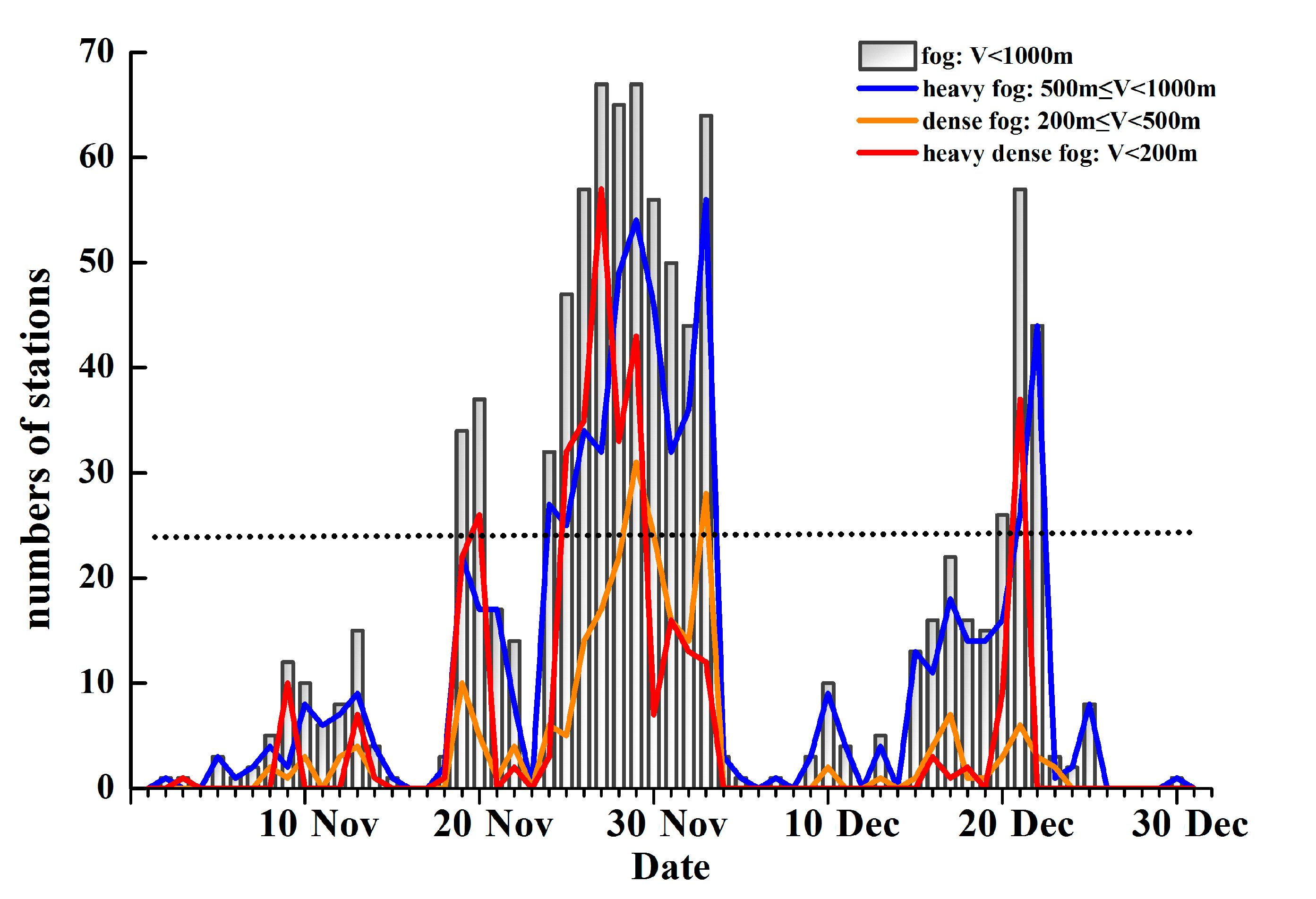
3.1. The Extremely Persistent Dense Fog Events Over Eastern China in the Late Autumn of 2018

In the late autumn of 2018, heavy fog events occurred persistently and frequently over Eastern China. Figure 1 shows the daily numbers of stations with the occurrence of fog (visibility less than 1000 m, bars), heavy fog (visibility between 1000 m and 500 m, blue line), dense fog (visibility less than and equal to 500 m and more than 200 m, orange line) and strong dense fog (SDF) (visibility less than 200 m, red line) events over Jiangsu Province in China. From 1 November to 30 December 2018, most of the days witnessed fog events, with at least one station seeing visibility of less than 1000 m for each day. The fog events from 24 November to 3 December are characterized by the strongest intensity and the longest duration in that year, with the daily visibility of at least 24 stations being less than 1000 m. This accounts for about one-third of all the 70 stations over Jiangsu Province. The number of stations with dense fog and SDF both reached the maximum in the late autumn of 2018. In particular, the SDF that covered at least 24 stations and persisted for five days from 25 to 29 November is rare and impressive. In the middle of November and the end of December, another two peaks of fog coverage appeared, but the durations for the respective fogs were short.

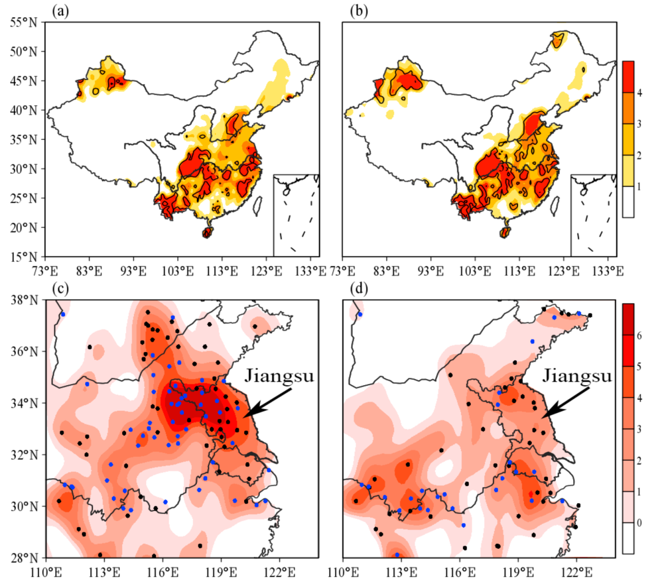
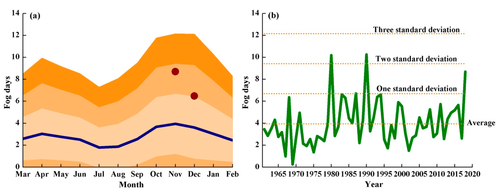
3.2. The Climate Anomalies of Fog Days in Late Autumn of 2018

Late autumn is a foggy season. The stations with high numbers of climatological fog days during November and December are located in most parts of Eastern China south of 40° N, and the southwestern and northwestern corners of China. Standard deviations of fog days exceeding 3.0 days are also located over the regions mentioned above (Figure 2a,b). It suggests that fog has a high possibility of occurrence and large interannual variability over those areas during late autumn.
In the late autumn of 2018, the fog days were above normal in many areas in Eastern China to the east of 110° E. In particular, the number of anomalous fog days was at least four days over the downstream area of the Yangtze River and the Yellow River in November 2018 (Figure 2c,d). The anomalous center, with values exceeding 8 days, appeared in central northern Jiangsu province over east China adjacent to the Yellow Sea where anomalies were above 3.0 standard deviations from the climatology (Figure 2c,d).
Figure 3a shows the annual cycles of fog occurrence from 1961 to 2017 averaged among 70 stations over the whole Jiangsu Province in China. The average annual value of fog days is 33.9 d at each station. The number of fog days varies with month; it has a double-peak structure, with the largest value of 4.0 d·year–1·station–1 occurring in November and another peak phase of 3.0 d·year–1·station–1 appearing in April. It is indicated that the fog events in Jiangsu occur mainly in boreal autumn, as the occurrence in this season accounts for approximately 30.03% of the annual fog occurrence, while the number in summer is small, only being 18.20% of the total. In November and December 2018, the average number of fog days over Jiangsu was 8.69 d and 6.47 d, respectively, and the anomalies were 1.0~2.0 standard deviations from the grand mean. The fog day in November also featured a remarkable interannual variability. In November 2018, the average number of anomalous fog days was 4.74 d, with an anomaly of 1.73 standard deviation departure from climatology. This was the third most fog days in November averaged over Jiangsu Province in China since 1961 and the most since the beginning of the 21st century (Figure 3b). It conflicted, to some extent, with the declining trend of fog days after the 1990s [30].
The heavy fog in November 2018 could be identified as an abnormal climatic event. What meteorological conditions are beneficial to the formation, development, and duration of fogs? What abnormal circulation anomalies and meteorological factors have significantly impacted the occurrence of this extremely persistent, dense fog? These two core questions motivate our research on the meteorological factors and abnormal circulations associated with this significant weather event.

3.3. Meteorological Conditions Conducive to the Persistent Dense Fog Events

The fog in the late autumn of 2018, with the strongest intensity, longest duration and most extensive coverage that year, persisted for 10 days from 24 November to 3 December, which is shown as the space between the two vertical lines in Figure 4a. During this period, the averaged daily visibility over Jiangsu Province in Eastern China shows a persistent lowest value of about 2 km. Numerous research has revealed that the occurrence of fogs is closely associated with certain meteorological factors [6,15,27,34]. The meteorological backgrounds can be classified into three categories: the dynamic, thermal and vapor conditions. The evolution of each meteorological factor is highly consistent with the development of daily visibility over Jiangsu Province in Figure 4b–f and Table 1. It significantly highlights the roles played by some kinds of meteorological condition.

3.3.1. Dynamical Conditions

Dynamically, fogs hardly occur under the background of strong surface winds or strong motions. Investigating the evolution of the absolute gradient of sea level pressure (SLP) as well as the 10 m and 1000 hPa winds in Figure 4b, it is revealed that a stronger (weaker) absolute gradient of SLP and a larger (smaller) surface wind velocity correspond well to higher (lower) visibility, suggesting highly positive correlation coefficients between the three dynamical factors and daily visibility. The correlation coefficients are 0.47, 0.51 and 0.51, respectively, all exceeding the 0.01 significance level (Table 1). During the most persistent dense fog events, the absolute gradient of SLP and the surface wind speed hit the minimum, hindering the outward transport of fog and favoring its development and persistence. On the other hand, increased visibility could be induced immediately due to strengthened surface winds. The maintenance and enhancement of lower visibility are also highly related to a weaker vertical motion and the mixing between the lower and middle troposphere (Figure 4c). The significant correlation coefficients of 1000 hPa vertical velocity and the vertical shear of horizontal winds between 500 and 850 hPa with daily visibility are 0.57 and 0.55, respectively (Table 1). It is indicated that the weak mixing or diffusion of air in the lower and middle troposphere is conducive to the congregation of fog droplets and the decline of visibility near the surface. It is apparent that a more stable and static atmosphere contributes to the formation and concentration of fog. Here, we calculated an index named the Eady growth rate (EGR), which measures the atmospheric baroclinicity [35,36,37]. The detailed equation of EGR is E G R = 0.31 | f N | d u d z , f is the Coriolis parameter, N is the Brunt–Väisälä frequency and u is the zonal winds. A higher EGR index means stronger activities of mid-latitude eddies and fluxes of transient eddy heat and momentum in the lower layer. Interestingly, the correlations of the daily 700 hPa and 1000 hPa EGR with visibility are quite opposite, which are 0.49 and −0.51, respectively, both exceeding the 0.01 significance level (Figure 4c and Table 1). The increased visibility associated with the rise of EGR at 700 hPa can be attributed to the enhancement of atmospheric baroclinicity in the lower troposphere, further intensifies the transport of transient eddy heat and momentum, and destroys the stability. Conversely, increased EGR at 1000 hPa will lead to lower visibility (Figure 4c). The underlying physical process might be the intensification of the turbulence in the boundary layer due to the increase of the transient eddy activities near the surface. The turbulent exchange implies a mixing of eddies of different origins, which promotes air saturation and fog formation [38]. Turbulence in the fog boundary layer (FBL) benefits the formation of fog [39]. Based on the view of Zhou and Ferrier [39] that the deeper a fog is, the stronger a turbulence intensity it can endure, persistent and appropriate turbulent activities are conducive to the long duration of fog in the fog events in the late autumn of 2018.
To sum up, weak outward horizontal transport, passive vertical diffusion in the lower troposphere and appropriate turbulence in FBL impose a critical impact on the formation and persistence of low visibility.

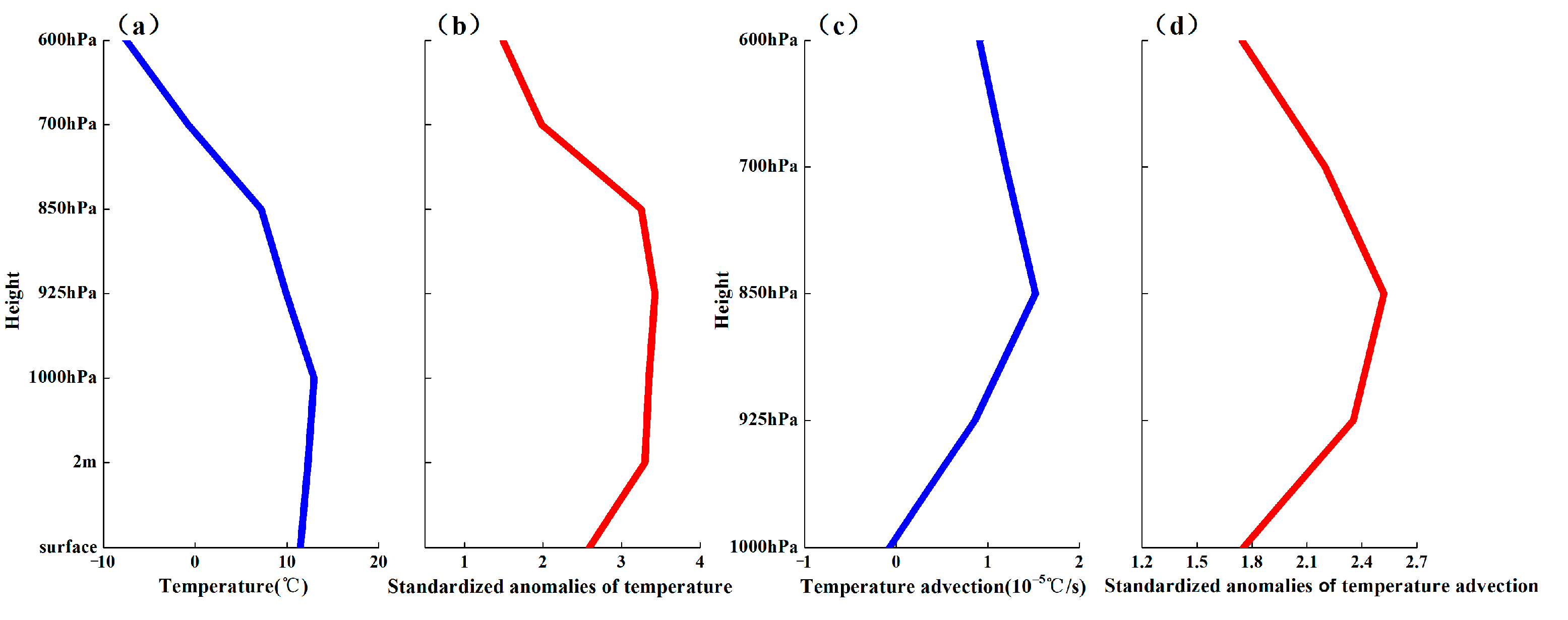
3.3.2. Thermal Conditions

The unique thermal conditions during the evolution of visibility are a major concern. Here, the daily evolutions of the vertical difference of temperature (VDT) between some layers are shown in Figure 4d, such as VDT between 925 and 1000 hPa, between 1000 hPa and 2 m, between 1000 hPa and the skin surface, and between 2 m and the skin surface. The correlation coefficients of the three calculation ways of VDT and the daily visibility are so significantly high (the correlation coefficients are −0.64, −0.68, −0.75, and −0.74 respectively in Table 1). This means that the consistent temperature inversion structure captures well the evolution of visibility. A stronger temperature inversion with a longer duration favors lower visibility, resulting in a persistent heavy fog. The formation of the inversion structure is connected with the relative cooling near the surface or the warm advection at the lower tropospheric layer. The two formation methods correspond to the two main types of fog, i.e., radiation fog, and advection fog. Both types were present in the persistent heavy fog events in 2018, as can be seen from the significant correlations of the intensity of inversion and 925-hPa temperature advection (the correlation coefficient is −0.45) with the evolution of visibility.

3.3.3. Vapor Conditions

Fog is composed of numerous tiny water droplets. Sufficient and saturated vapor is, as revealed, a prerequisite for the formation and persistence of fog, which means that the absolute and relative humidity conditions are both indispensable to fog events. The significant correlations between the humidity factors (the 1000 hPa specific humidity, 2 m dew point, 1000 hPa relative humidity and the dewpoint deficit at 2 m) and visibility indicate that more vapor and a higher degree of saturation near the surface are favorable for water vapor condensation, thus helping form or enhance the fog phenomena (Figure 4e–f and Table 1).
The above analyses confirm that the persistent dense fog in the late autumn of 2018 was well configured by certain meteorological conditions such as weak dynamic progress, strong inversion and saturated air near the surface. If not disturbed, the duration or intensification of these conditions will further promote the development of fogs.

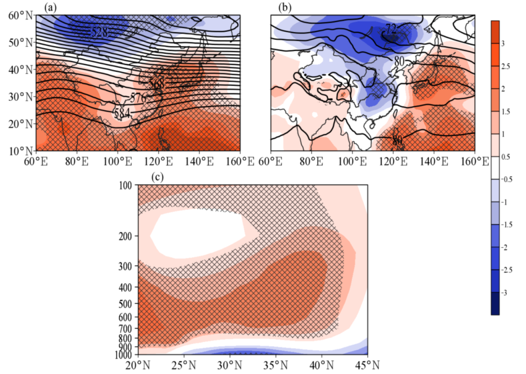
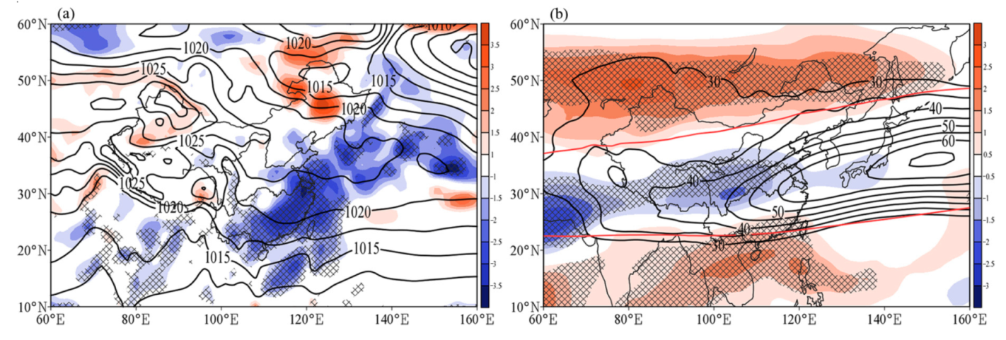
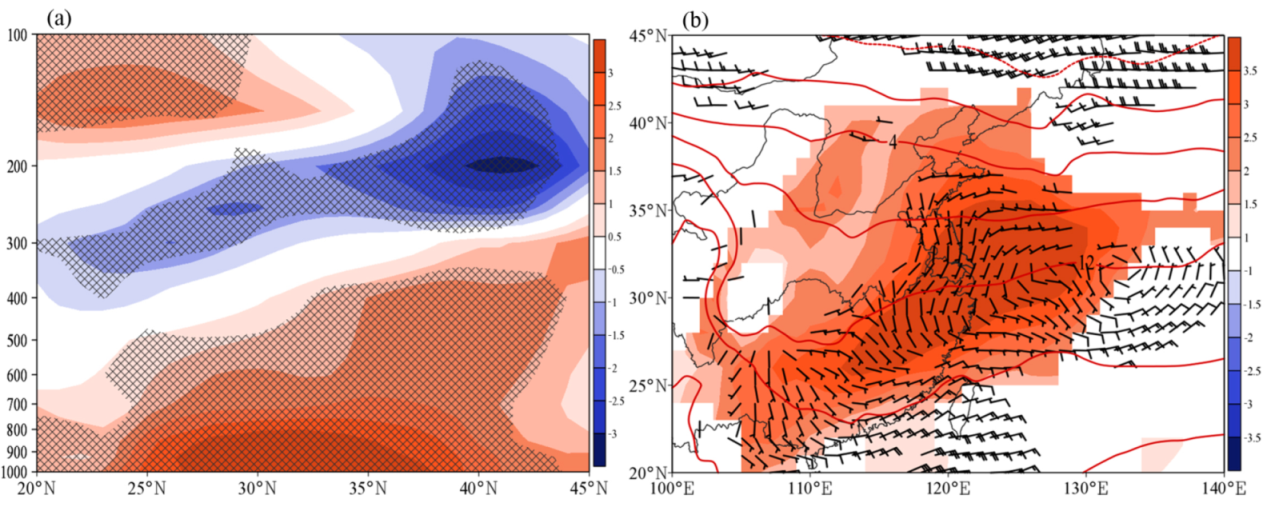
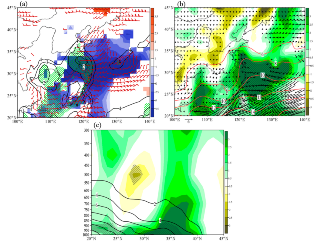
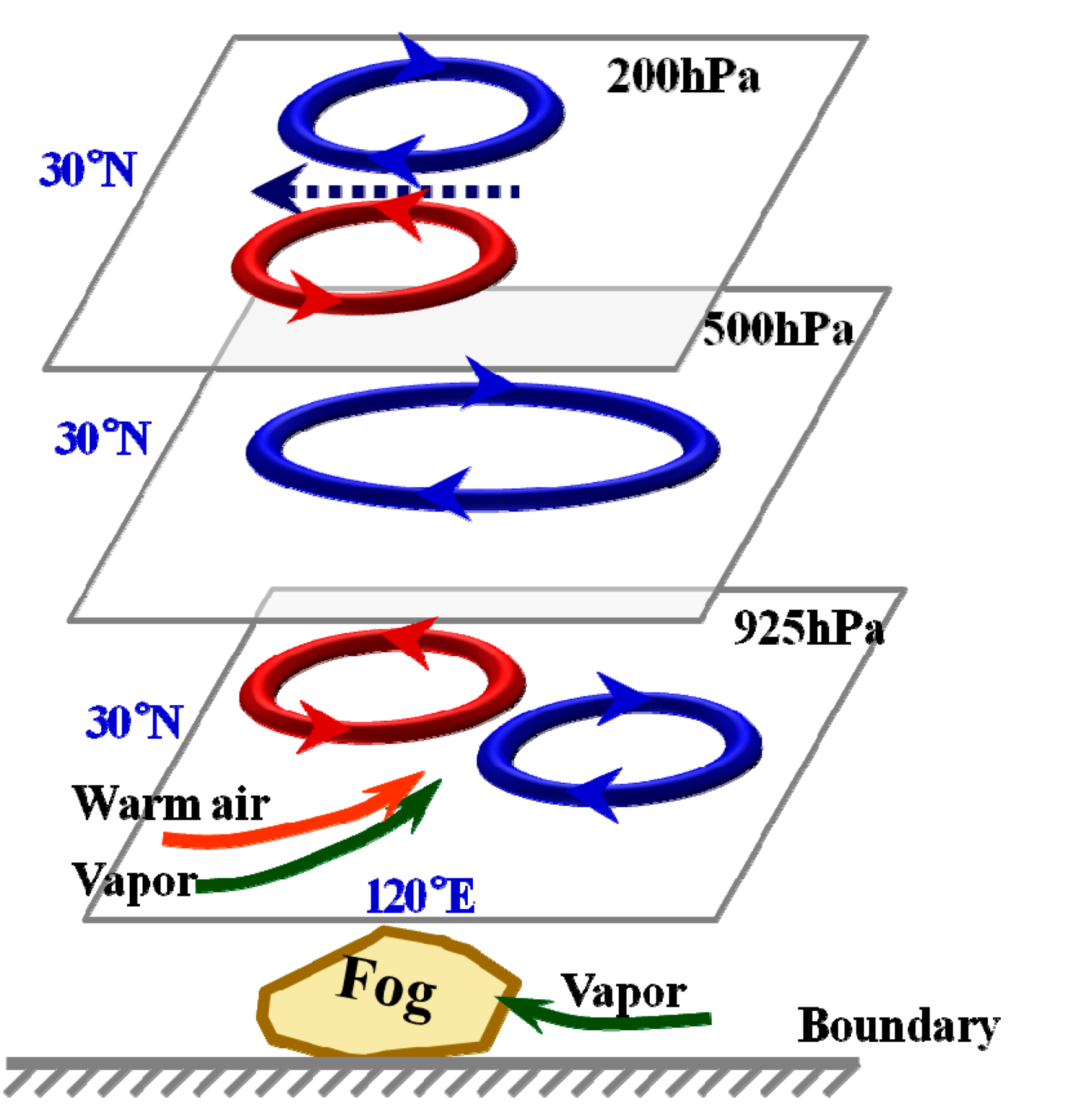
3.4. The Associated Anomalous Atmospheric Circulations

In this section, attention is paid to the anomalous atmospheric background that provides favorable metrological conditions for those extreme fog events with long duration and strong intensity. A deep understanding of the anomalous atmospheric circulations acts as the foundation for the short-term, medium-term and even sub-seasonal forecasts of fog, and is vital to unraveling the underlying physical processes behind the impact of extra-forcings (such as sea surface temperature) on fog at some timescales. The composite analysis and the Student’s t-test analysis of the standardized anomalies [40] were conducted on all the circulation fields for fog days from 24 November to 3 December in 2018.

3.4.1. Anomalous Dynamic Circulations

Figure 5a,b depict the distributions of the composite 500 and 925 hPa original and anomalous geopotential heights (GH). During the fog days, a trough with a smaller magnitude lies over coastal East Asia, which is accompanied by universally positive GH anomalies south to 45° N, especially over Eastern China in the middle troposphere (Figure 5a). Meanwhile, in the lower layer, there exist abnormally weaker GH over land and stronger GH over the sea to the east of 105° E, resulting in anomalous northward flows along with Eastern China according to the theory of geostrophic wind equilibrium (Figure 5b). The East Asian trough in the middle troposphere and the East Asian winter monsoon in the lower troposphere are obviously weakened so that the invasion of cold air to Eastern China is effectively curbed, and the anomalous southerly flows transport more heat and vapor to Eastern China in the lower troposphere. The corresponding anomalous southerly winds are also presented in the troposphere above 900 hPa (the figure is omitted). In the vertical section of composite GH standard deviations across 120° E (Figure 5c), significant negative GH anomalies only appear at the shallow lower layers under 900 hPa, while significant positive GH anomalies are present almost in the entire troposphere above 900 hPa. It is suggested that the occurrence of the local meteorological conditions closely correlated with the persistent dense fog can be attributed to the certain persistent anomalous large-scale circulation pattern. Anomalous circulation signals characterized with the weaker cold high and the absolute gradient of SLP emerge at the boundary layer. This induces a decline in wind velocity near the surface over Eastern China (Figure 5c and Figure 6a). Moreover, circulation anomalies also occur in the higher troposphere. For example, it is shown that during the extremely persistent dense fog events in 2018, the East Asian jet stream (EAJS) at 200 hPa was markedly broadened and weakened with the occurrence of westerly anomalies north to 40° N and south to 20° N and easterly anomalies between 20~40° N. The northern (southern) flank (the wind velocity is 30 m·s−1) shifted northward (southward) from the climatological location of EAJS (Figure 6b). The northward-shifted EAJS became so apparent that it could hinder the meridional invasion of cold air from high latitudes [41,42], and the weakened westerly jet between 20~40° N might attenuate the baroclinicity belt in the troposphere via wave-zonal flow interactions [36]. Considering the northward and southward shifts of the jet’s flanks, and the weakness of the jet’s core, the East Asian trough, and the East Asian winter monsoon, it might be speculated that the entire circulation structure is loosened, favoring a static and stable weather condition and hampering any vortex activities or cold air invasion.

3.4.2. Anomalous Thermal Circulations

Matched well with the significant GH anomalies in the vertical section according to the theory of static equilibrium and the air state equation, pronounced warm temperature anomalies fill the whole middle and lower troposphere from 1000 hPa to 400 hPa (Figure 7a). This indicated that the air temperature rose over Eastern China from 24 November to 3 December in 2018. Figure 8a,b shows the vertical distributions of regional and time-averaged temperature and standard temperature anomalies. Among the generally positive temperature anomalies with height in the whole troposphere under 400 hPa, the increases of air temperature at 925 and 850 hPa are the most significant with over 3.0 standard deviation anomalies, presenting an obvious inversion in the profiles of regional and time-averaged standard temperature anomaly and a nearly isothermal layer in those of the actual temperature. The vertical structure of inversion below 850 hPa is intimately related to the significant negative GH anomalies under 900 hPa based on the theory of static equilibrium. As the anomalous inversion in the lower troposphere enhances the stability of the near-surface atmosphere, it contributes to the formation and maintenance of fogs. It is apparent that the structure of the inversion is mainly attributed to the warm advection at 925 and 850 hPa associated with the southerly flows. As seen in the composite 925 hPa winds and air temperature averaged from 24 November to 3 December in 2018 (Figure 7b), in Eastern China, especially over Jiangsu Province, the northward wind is nearly perpendicular to the isotherm, inducing obvious warm temperature advection anomalies. The anomaly centers of the standard deviations of temperature and temperature advection are above 3.0, representing an unusual and even rare departure from average conditions (Figure 7). Below 850 hPa, the distributions of regional and time-averaged temperature advection and the standard deviations at different heights (Figure 8c,d) both show a distinct inversion. The standard deviation anomalies of temperature advection at 850 hPa are more than 2.5, indicating uncommon thermal circulation in the fog days compared with the climatology at the lower troposphere.

3.4.3. Anomalous Vapor Circulations

In the boundary air, weakening of the surface wind velocity during fog days (Figure 9a) is closely related to the southerly wind anomalies in the lower troposphere going along with the weakened East Asian winter monsoon (Figure 5 and Figure 6a). The weakened velocity at the surface further hampers the export of fogs. Meanwhile, east of Eastern China lies a vast ocean and the central place of these fog events, Jiangsu Province, is adjacent to the Yellow Sea. The easterly wind can transport abundant vapor from the sea. The composite specific humidity advection is over 3.0 and exceeds the 0.01 significance level over most regions in East China (Figure 9b). It contributes to an anomalous persistent supplement for high humidity at the near-surface layer. The anomalous saturated and humid conditions over Eastern China are also presented significantly. The dew point depression of 2 m is less than 3 °C. The specific humidity is more than 6 g/kg with a wave ridge of the specific humidity line along the coast in the boundary during the fog days (Figure 9a,b). The sustained weak easterly winds, abundant vapor transport, and condensation in the boundary are the indispensable circulation factors for the formation, enhancement, and maintenance of fogs over Eastern China. Moreover, due to the anomalous southerly winds, the positive humidity anomalies at the middle latitudes are distributed to the whole troposphere (Figure 9c). Figure 9c shows the center of composite original specific humidity across 120° E at the whole lower troposphere is more than 6 g/kg and just over 32° N~35° N in the middle latitudes. The composite standard deviations of specific humidity over that region are mostly over 3.0, indicating the rarity of the vapor during the fog events.
Overall, the anomalous atmospheric circulation pattern in the entire troposphere during the extremely persistent dense fog events over Eastern China in the late autumn of 2018 can be concluded in the schematic diagram shown in Figure 10. During the fog days, the anticyclonic circulation anomaly in the north of EAJS and the cyclonic circulation anomaly in the south of EAJS broaden and weaken the core of the jet over Eastern China. The East Asian trough with the anticyclonic circulation anomaly at 500 hPa is effectively weakened. Meanwhile, in the lower layer in Eastern China, the cyclonic and anticyclonic circulation anomalies occur in the west and the east, respectively, resulting in the weakening of East Asian winter monsoon and the enhancement of the anomalous southerly flows that transport abnormal warm and wet air to Eastern China. The abnormal circulation pattern in the troposphere hampers the occurrence of any vortex activities or cold air invasion. The atmosphere is inclined to be stable, and the vapor condensation and adequate vapor amount provide the necessary metrological conditions for fog as well. Correspondingly, the sustained anomalous northward wind at the lower troposphere and anomalous westward wind in the near-surface both intensify the vapor supplement.
It is noteworthy that the numbers of the standardized anomalies of 1000–200 hPa height, temperature, wind, and moisture fields during these fog days all significantly depart from climatology for that locale and time of the season. It has been further demonstrated that the persistent dense fogs over Eastern China in the late autumn of 2018 are a significant unusual weather event with extreme synoptic-scale departures from normal [32].

4. Conclusions and Discussion

Global warming is generally expected to intensify extreme weather events [43]. Meteorological events directly impact processes taking place at the Earth’s surface. Fog with low visibility is a kind of hazardous weather. Fog impacts transportation difficulties, air quality and public health [4,44].
From mid–late November to early December in 2018, extremely persistent dense fog events with long duration, low visibility, and extensive coverage occurred in Eastern China, especially in Jiangsu Province, a coastal province on the shore of the Yellow Sea. The heavy fog weather had an unprecedented severe effect on the road and air transport and was widely reported at home and abroad.
From 24 November to 3 December in 2018, the fog events were characterized by the strongest intensity and the longest duration for that year. At least 24 stations, about one-third of all the 70 stations over Jiangsu Province, observed visibilities of less than 1000 m during this period. In particular, the SDF (visibility less than 200 m) that covered at least 24 stations and persisted for five days from 25 November to 29 November was rare and impressive. The fog days averaged over Jiangsu in November and December 2018 were 8.69 d and 6.47 d, respectively, and compared with the climatology of fogs in late autumn, the anomalies were 1.0~2.0 standard deviations from the grand mean. The number of fog days in November 2018 ranked the third-highest since 1961 and the first since the beginning of the 21st century despite a declining trend after the 1990s.
Undoubtedly, the evolution of each meteorological factor conducive to fog is consistent with that of the daily visibility over Jiangsu Province. To sum up, the common favorable metrological conditions include weak dynamic progress, stable atmospheric stratification, strong inversion in the lower troposphere, and affluent and saturated air near the surface. For instance, dynamic processes such as weaker outward horizontal transport, more passive vertical diffusion in the lower troposphere and suitable turbulent conditions in the fog boundary layer impose a critical impact on the development and persistence of lower visibility. During the fog days, the formation and maintenance of the inversion structure, an important factor for the stability of the atmosphere, are connected with the relative cooling near the surface and the warm advection at the lower tropospheric layer. It should also be emphasized that the absolute and relative humidity conditions are both indispensable for such persistent dense fogs with extensive coverage.
The persistent dense fogs over Eastern China in the late autumn of 2018 are not only an unusual weather event with synoptic-scale departures from normal but also a significantly abnormal climatic event with the third most duration days since 1961. The anomalous atmospheric circulation pattern in the entire troposphere, which matches the extreme fogs well, is analyzed in detail as follows. During the fog days, the East Asian jet stream broadened and the core of the jet over Eastern China weakened associated with the anticyclonic circulation anomaly in the north of EAJS and the cyclonic circulation anomaly in its south. In the middle troposphere, the East Asian trough with the anticyclonic circulation anomaly at 500 hPa was present in a weaker amplitude. In the lower layer in Eastern China, the cyclonic and anticyclonic circulation anomalies in the west and the east resulted in weakened East Asian winter monsoon. All the abnormal circulation conditions in the troposphere were inclined to hamper vortex activities or cold air invasion and thus intensify the atmospheric stability. By confining the affluent and saturated air near the surface, the sustained anomalous northward wind at the lower troposphere and anomalous westward wind in the near-surface play a great part in the vapor supplement. The revelation of anomalous circulation and abnormal features of synoptic systems that provide favorable meteorological conditions for fog effectively enhances the capability to forecast extreme fog in the short-term, medium-term and even sub-seasonal timescales. Although this research only deals with a case study, our findings of the abnormal features of fog and the associated circulation situation based on synoptic-scale departures from normal lay the foundation for unraveling the underlying physical processes behind the impact of extra-forcing on fog at interannual or even longer timescales. In future work, more historical rare fog cases will be researched to further verify our robust schematic diagram.
From a synoptic point of view, the dense fog events over Eastern China in the late autumn of 2018 could be described as an extreme or a rare event. There are still many difficulties in producing accurate and effective forecasts for similar severe fog events that are characterized by long duration, strong intensity and extensive coverage on the medium-term and even sub-seasonal timescales. It is necessary to find objective methods or standards to rank such fog events, and their predictability needs to be further investigated in future studies.

Author Contributions

The study was completed with cooperation among all the authors: Conceptualization, S.C., D.L. and Z.K.; data and methodology, Y.S.; writing—review and editing, S.C. and D.L.; visualization, M.L.; project administration, Z.K. and D.L. All authors have read and agreed to the published version of the manuscript.

Funding

This work was jointly supported by the National Key Project of MOST (2016YFC0203303 and 2016YFC0201903), the open fund by the Key Laboratory for Aerosol–Cloud–Precipitation of CMA–NUIST in China (KDW1801), the National Natural Science Foundation of China (91544231 and 41575135), and the Jiangsu meteorological bureau key fund (KZ201801).

Institutional Review Board Statement

Not applicable.

Informed Consent Statement

Informed consent was obtained from all subjects involved in the study.

Data Availability Statement

The circulation data is publicly available datasets analyzed in this study. The data can be found here: https://apps.ecmwf.int/datasets/data/interim-full-daily/levtype=sfc/. Restrictions apply to the availability of the fog observation data. Data was obtained from China Meteorological Administration and are available from the authors of this paper with the permission of China Meteorological Administration.

Conflicts of Interest

The authors declare no conflict of interest.

References

  1. Jiusto, J.E. Fog structure. In Clouds, Their Formation, Optical Properties and Effect; Hobbs, P.V., Deepak, A., Eds.; Academic Press: New York, NY, USA, 1981; pp. 187–239. [Google Scholar]
  2. Nemery, B.; Hoet, P.H.; Nemmar, A. The Meuse Valley fog of 1930, an air pollution disaster. Lancet 2001, 357, 704–708. [Google Scholar] [PubMed]
  3. Houssos, E.E.; Lolis, C.J.; Bartzokas, A. The main characteristics of atmospheric circulation associated with fog in Greece. Nat. Hazard. Earth Syst. 2009, 9, 1857–1869. [Google Scholar]
  4. Gautam, R.; Singh, M.K. Urban heat island over Delhi Punches Holes in widespread fog in the Indo–Gangetic Plains. Geophys. Res. Lett. 2018, 45, 1114–1121. [Google Scholar]
  5. Li, Z.H.; Yang, J.; Shi, C.E. The Physics of Regional Dense Fog; China Meteor Press: Beijing, China, 2008; p. 160. (In Chinese) [Google Scholar]
  6. Ye, H. The influence of air temperature and atmospheric circulation on winter fog frequency over Northern Eurasia. Int. J. Climatol. 2009, 29, 729–734. [Google Scholar]
  7. Emmons, G.; Montgomery, R.B. Notes on the physics of fog formation. J. Meteorol. 1947, 4, 206. [Google Scholar]
  8. Choularton, T.W.; Fullarton, G.; Latham, J.; Mill, C.S. A field study of radiation fog in Meppen, West Germany. Q. J. R. Meteorol. Soc. 1981, 107, 381–394. [Google Scholar]
  9. Brown, R.; Roach, W.T. The physics of radiation fog, II–a numerical study. Q. J. R. Meteorol. Soc. 1976, 102, 335–354. [Google Scholar]
  10. Herckes, P.; Marcotte, A.R.; Wang, Y.; Collett, J. Fog composition in the Central Valley of California over three decades. Atmos. Res. 2015, 151, 20–30. [Google Scholar]
  11. Degefie, D.T.; El–Madany, T.S.; Hejkal, J.; Held, J. Microphysics and energy and water fluxes of various fog types at SIRTA, France. Atmos. Res. 2015, 151, 162–175. [Google Scholar]
  12. Stolaki, S.; Haeffelin, M.; Lac, C.; Dupont, J.C.; Elias, T.; Masson, V. Influence of aerosols on the life cycle of a radiation fog event. A numerical and observational study. Atmos. Res. 2015, 151, 146–161. [Google Scholar]
  13. Guedalia, D.; Bergot, T. Numerical Forecasting of Radiation Fog. Part II, A Comparison of Model Simulation with Several Observed Fog Events. Mon. Weather Rev. 1994, 122, 1231–1246. [Google Scholar] [CrossRef] [Green Version]
  14. Houssos, E.E.; Lolis, C.J.; Gkikas, A.; Hatzianastassiou, N.; Bartzokas, A. On the atmospheric circulation characteristics associated with fog in Ioannina, north–western Greece. Int. J. Climatol. 2011, 32, 1847–1862. [Google Scholar] [CrossRef]
  15. Zhang, R.H.; Li, Q.; Zhang, R.N. Meteorological conditions for the persistent severe fog and haze event over eastern China in January 2013. Sci. China Earth Sci. 2014, 57, 26–35. [Google Scholar]
  16. Telišeli–Prtenjak, M.; Klaić, M.; Cuxart, J.; Jerirević, A. The interaction of the downslope winds and fog formation over the Zagreb area. Atmos. Res. 2017, 214, 213–227. [Google Scholar] [CrossRef]
  17. Willett, H.C. Fog and Haze, Their Causes, Distribution, and Forecasting. Mon. Weather Rev. 1928, 56, 435–468. [Google Scholar] [CrossRef]
  18. Meyer, M.B.; Lala, G.G. Climatological aspects of Radiation Fog Occurrence at Albany, New York. J. Clim. 1990, 3, 577–586. [Google Scholar] [CrossRef] [Green Version]
  19. Bergot, T.; Guedalia, D. Evaluation of the success of fog forecasting by a numerical model. Meteorologie 1996, 14, 27–35. [Google Scholar]
  20. Van der Velde, I.R.; Steeneveld, G.J.; Wichers Schreur, B.G.J.; Holtslag, A.A.M. Modeling and Forecasting the Onset and Duration of Severe Radiation Fog under Frost Conditions. Mon. Weather Rev. 2010, 138, 4237–4253. [Google Scholar] [CrossRef]
  21. Steeneveld, G.J.; Ronda, R.J.; Holtslag, A.A.M. The Challenge of Forecasting the Onset and Development of Radiation Fog Using Mesoscale Atmospheric Models. Bound. Lay. Meteorol. 2015, 154, 265–289. [Google Scholar] [CrossRef]
  22. Herman, G.R.; Schumacher, R.S. Using Reforecasts to Improve Forecasting of Fog and Visibility for Aviation. Weather Forecast. 2016, 31, 467–482. [Google Scholar] [CrossRef]
  23. Meng, Y.J.; Wang, S.Y.; Zhao, X.F. An analysis of air pollution and weather conditions during heavy fog days in Beijing area. Meteorl. Mon. 2000, 26, 40–42. [Google Scholar]
  24. Liu, X.N.; Zhang, H.Z.; Li, Q.X.; Zhu, Y.J. Preliminary research on the climatic characteristics and change of fog in China (in Chinese). J. Appl. Meteorol. Sci. 2005, 16, 220–229. [Google Scholar]
  25. Lin, J.; Yang, G.M.; Mao, D.Y. Spatial and temporal characteristics of fog in China and associated circulation patterns (in Chinese). Clim. Environ. Res. 2008, 13, 171–181. [Google Scholar]
  26. Wu, D.; Bi, X.Y.; Deng, X.J.; Li, F.; Tan, H.B.; Liao, G.L.; Huang, J. Effect of atmospheric haze on the deterioration of visibility over the Pearl River Delta. Acta Meteorol. Sin. 2007, 21, 215–223. [Google Scholar]
  27. Ding, Y.H.; Liu, Y.J. Analysis of long–term variations of fog and haze in China in recent 50 years and their relations with atmospheric humidity. Sci. China Earth Sci. 2014, 57, 36–46. [Google Scholar] [CrossRef]
  28. Ma, N.; Zhao, C.S.; Chen, J.; Xu, W.Y.; Yan, P.; Zhou, X.J.A. novel method for distinguishing fog and haze based on pm2.5, visibility, and relative humidity. Sci. China Earth Sci. 2014, 57, 2156–2164. [Google Scholar] [CrossRef]
  29. Zhang, X.Y.; Wang, Y.Q.; Niu, T.; Zhang, X.C. Atmospheric aerosol compositions in China, spatial/temporal variability, chemical signature, regional haze distribution and comparisons with global aerosols. Atmos. Chem. Phys. 2012, 12, 779–799. [Google Scholar] [CrossRef] [Green Version]
  30. Sun, Y.; Ma, Z.F.; Niu, T.; Fu, R.Y.; Hu, J.F. Characteristics of climate change with respect to fog days and haze days in China in the past 40 years(in Chinese). Clim. Environ. Res. 2013, 18, 397–406. [Google Scholar]
  31. Wu, D. More discussions on the differences between haze and fog in city (in Chinese). Meteorl. Mon. 2006, 32, 9–15. [Google Scholar]
  32. Hart, R.E.; Grumm, R.H. Using Normalized Climatological Anomalies to Rank Synoptic–Scale Events Objectively. Mon. Weather Rev. 2001, 129, 2426–2442. [Google Scholar] [CrossRef]
  33. Dee, D.P.; Uppala, S.M.; Simmons, A.J.; Berrisford, P.; Poli, P.; Kobayashi, S.; Andrae, U.; Balmaseda, M.A.; Balsamo, G.; Bauer, P.; et al. The ERA-interim reanalysis, configuration and performance of the data assimilation system. Q. J. R. Meteorol. Soc. 2011, 137, 553–597. [Google Scholar] [CrossRef]
  34. Liu, D.Y.; Yang, J.; Niu, S.J.; Li, Z.H. On the evolution and structure of a radiation fog event in Nanjing. Adv. Atmos. Sci. 2011, 28, 223–237. [Google Scholar] [CrossRef]
  35. Eady, E.T. Long waves and cyclone waves. Tellus 1949, 1, 33–52. [Google Scholar] [CrossRef] [Green Version]
  36. Hoskins, B.J.; Valdes, P.J. On the existence of storm–tracks. J. Atmos. Sci. 1990, 47, 1854–1864. [Google Scholar] [CrossRef]
  37. Lindzen, R.S.; Farrell, B. A simple approximate result for the maximum growth rate of baroclinic instabilities. J. Atmos. Sci. 1980, 37, 1648–1654. [Google Scholar] [CrossRef] [Green Version]
  38. Rodhe, B. The effect of turbulence on fog formation. Tellus 1962, 14, 49–86. [Google Scholar] [CrossRef] [Green Version]
  39. Zhou, B.; Ferrier, B.S. Asymptotic Analysis of Equilibrium in Radiation Fog. J. Appl. Meteorol. Clim. 2008, 47, 1704–1722. [Google Scholar] [CrossRef]
  40. Grumm, R.H.; Hart, R.E. Standardized Anomalies Applied to Significant Cold Season Weather Events, Preliminary Findings. Weather Forecast. 2001, 16, 736–754. [Google Scholar] [CrossRef]
  41. Wang, J.; Zhao, Q.H.; Zhu, Z.W.; Qi, L.; Wang, J.X.L.; He, J.H. Interannual variation in the number and severity of autumnal haze days in the Beijing–Tianjin–Hebei region and associated atmospheric circulation anomalies. Dyn. Atmos. Ocean. 2018, 84, 1–9. [Google Scholar] [CrossRef]
  42. Yin, Z.C.; Wang, H.J. Role of atmospheric circulations in haze pollution in December 2016. Atmos. Chem. Phys. 2017, 17, 11673–11681. [Google Scholar] [CrossRef] [Green Version]
  43. Diffenbaugh, N.S. Verification of extreme event attribution: Using out-of-sample observations to assess changes in probabilities of unprecedented events. Sci. Adv. 2020, 6, eaay2368. [Google Scholar] [CrossRef] [PubMed] [Green Version]
  44. Kim, H.; Collier, S.; Ge, X.; Xu, J.; Sun, Y.; Jiang, W.; Wang, Y.; Herckes, P.; Zhang, Q. Chemical processing of water-soluble species and formation of secondary organic aerosol in fogs. Atmos. Environ. 2019, 200, 158–166. [Google Scholar] [CrossRef]
Figure 1. The daily numbers of stations with the occurrence of fog (mean daily visibility less than 1000 m, bars), heavy fog (visibility less than 1000 m and more than 500 m, blue line), dense fog (visibility less than and equal to 500 m and more than 200 m, orange line) and strong dense fog (visibility less than 200 m, red line) events over Jiangsu Province in China. The dotted line denotes 24 stations, which are about one-third of all the 70 stations over Jiangsu Province.
Atmosphere 12 00111 g001
Figure 2. (a) The climatological fog days in November averaged from 1961 to 2017 (shaded) in China. Standard deviations exceeding 3.0 days are marked by contours; (b) as in (a), but for December; (c) the anomalous fog days (shaded) and the stations that anomalies exceeding 2.0 (black dots)/3.0 (black dots) standard deviations in November 2018 in China; (d) as in (c), but for December. The units of all shaded and contours are days. The two lines on the China map are the Yellow River (line in the northern) and Yangtze River (line in the southern). The boundary of Jiangsu Province, China is marked in (c,d).
Atmosphere 12 00111 g002
Figure 3. (a) The climatological annual cycles of fog days (dark blue line) averaged from 1961 to 2017 over Jiangsu Province in China (the boundary of is Jiangsu Province marked in Figure 2c). The filled lines from light orange to dark orange represent ±1, ±2 and 3 standard deviations among the measured sites. The red solid circles mark the fog days of November and December in 2018. (b) The interannual variations of fog days in November averaged over Jiangsu Province in China from 1961 to 2018. The four dotted lines denote the average fog days and the fog days of one to three standard deviations.
Atmosphere 12 00111 g003
Figure 4. (a)The daily evolution of the number of stations with the occurrence of fog and the daily averaged visibility over Jiangsu Province in China (The boundary of is Jiangsu Province marked in Figure 2c) and (bf) the daily evolution of different kinds of related meteorological factors. All variabilities are averaged over the area of 115° E~122° E, 30° N~35° N. The parameters include (1) dynamical conditions (b,c): 10 m and 1000 hPa wind speed (units: m·s−1), absolute gradient of SLP (units: 10−3 Pa·m−1) (b), 1000 hPa vertical velocity (units: 10−2 Pa·s−1), 700 and 1000 hPa EGR (units: day−1), and vertical shear of winds between 500 and 850 hPa (units: m·s−1) (c); (2) thermal conditions (d): vertical difference of temperature (VDT) between 1000 hPa and 2 m, between 925 and 1000 hPa, between 1000 hPa and the skin surface, and between 2 m and the skin surface (units: °C), and the 925 hPa temperature advection (units: 10−5 °C·s−1); (3) vapor conditions (e,f): 1000 hPa specific humidity (units: g·kg−1), dew point of 2 m (units: °C) (e), the dew point depression of 2 m (units: °C) and 1000 hPa relative humidity (units: %) (f). All numbers in the brackets in the legend of each line-layers are the correlation coefficients of each meteorological factor with the averaged daily visibility over Jiangsu Province in China. The period between the two vertical lines is from 24 November to 3 December.
Atmosphere 12 00111 g004
Figure 5. (a) The composite of original 500 hPa geopotential height (GH) (contours, unit: gpm) and standard anomalies of GH (shaded) from 24 November to 3 December in 2018. (b) is the same as in (a) but for 925 hPa GH. (c) The vertical section of composite standard anomalies of GH across 120° E. The crossed area in each panel denotes anomalies exceeding the 0.01 significance level.
Atmosphere 12 00111 g005
Figure 6. (a) The composite of original sea level pressure (SLP) (contours, unit: hPa) and standard anomalies of the absolute gradient of SLP (shaded) from 24 November to 3 December in 2018. (b) The composite analysis of original 200 hPa u winds (Only values more than 30 m·s−1 is shown as contours) and standard anomalies of 200 hPa u winds (shaded) from 24 November to 3 December in 2018. The red line in (b) is the climatological u = 30 m·s−1 at 200 hPa. The crossed area in each panel denotes anomalies exceeding the 0.01 significance level.
Atmosphere 12 00111 g006
Figure 7. (a) The vertical section of composite standard anomalies of air temperature across 120° E. The crossed area in each panel denotes anomalies exceeding the 0.01 significance level. (b) The composite of original winds (Only anomalies exceeding the 0.01 significance level are shown as shafts; units: m·s−1), original temperature (contours, units: °C) and standard anomalies of temperature advection (Only the composite standard anomalies exceeding the 0.10 significance level are shaded) at 925 hPa.
Atmosphere 12 00111 g007
Figure 8. The profiles of the vertical distribution of composite (a) temperature, (b) standard anomalies of temperature, (c) temperature advection, and (d) standard anomalies of temperature advection averaged over the area of 115–122° E, 30–35° N in Eastern China from 24 November to 3 December in 2018.
Atmosphere 12 00111 g008
Figure 9. (a) The composite 10-m winds (only anomalies exceeding the 0.01 significance level are shown as shafts, units: m·s−1), the standard deviation of 10 m wind velocity standard deviation of 10 m wind velocity (only anomalies exceeding the 0.01 significance level are shaded), and the 2 m dew point depression (contours are values less than 4 °C). The green oblique line area denotes the anomalies of 2-m dew point depression exceeding the 0.01 significance level. (b) The composite 1000 hPa specific humidity (contours are values more than 6g·kg−1), 1000 hPa vapor flux (only anomalies exceeding the 0.01 significance level are shown as vectors, units: 10−2g·kg−1·m·s−1), and standard deviation of specific humidity advection (shaded). The crossed area denotes anomalies of specific humidity advection exceeding the 0.01 significance level. (c) The vertical section of composite original specific humidity (contours are the values more than 2g·kg−1) and standard deviation of specific humidity (shaded) across 120° E. The crossed area denotes anomalies of specific humidity exceeding the 0.01 significance level.
Atmosphere 12 00111 g009
Figure 10. Schematic diagram of the anomalous atmospheric circulations during the extremely persistent dense fog events over Eastern China in the late autumn of 2018.
Atmosphere 12 00111 g010
Table 1. The summarization of the correlation coefficients of kinds of meteorological dynamical, thermal and vapor factors with the daily averaged visibility over Jiangsu Province in China. All the correlations exceed the 0.01 significance level.
ConditionsParametersThe Correlation Coefficient
dynamical10 m wind speed0.51
1000 hPa wind speed0.51
the absolute gradient of sea level pressure0.47
1000 hPa vertical velocity0.57
700 hPa Eady growth rate (EGR)0.49
1000 hPa EGR−0.51
vertical shear of winds between 500 and 850 hPa0.55
thermalvertical difference of temperature (VDT) between 1000 hPa and 2 m−0.68
VDT between 925 and 1000 hPa−0.64
VDT between 1000 hPa and the skin surface−0.75
VDT between 2 m and the skin surface−0.74
925 hPa temperature advection−0.45
vapor1000 hPa specific humidity−0.48
The 2 m dew point−0.54
the 2 m dew point depression0.56
1000 hPa relative humidity−0.37
Publisher’s Note: MDPI stays neutral with regard to jurisdictional claims in published maps and institutional affiliations.

