The Temporal Evolution of PM_2.5 Pollution Events in Taiwan: Clustering and the Association with Synoptic Weather

Abstract

This study conducted a cluster analysis on the fine particulate matter (PM_2.5) data over Taiwan from 2006 to 2015 and diagnosed their association with the synoptic weather patterns. Five clusters are identified via a hierarchical clustering algorithm; three of them correspond to severe events, each with a distinct pattern of temporal evolution within the 240-h window. The occurrence of the different clusters exhibits strong seasonal variation. Two of the polluted clusters are more frequently associated with weak synoptic weather, while the other one is related to northeasterly winds and fronts. Detailed case studies show that the weather patterns’ temporal evolutions clearly modulate the transition among various pollution clusters by influencing the changes in local circulation and atmospheric stability. In winter, the clusters characterizing severe PM_2.5 pollution events occur when Taiwan is influenced by persistent weak synoptic condition, while in autumn, the long-range transport by strong northerly winds leads to the occurrence of severe PM_2.5 pollution. The current results shed light on the potential of combining the data-driven approach and the numerical weather forecasting model to provide extended range forecasts of local air pollution forecasts.

1. Introduction

Pollution of fine particulate matter with a diameter smaller than 2.5 microns (PM_2.5) is a crucial environmental and public health issue in Taiwan, and the influence of the weather systems on PM_2.5 pollution has been studied extensively. When major pollution events occur, the polluted areas can exhibit areal mean PM_2.5 concentrations around 40 μg m⁻³, with maximum values approaching 80 μg m⁻³ [1]. The PM_2.5 concentrations are contributed by both local emission sources and long-range transport, and the severe PM_2.5 pollution conditions often occur from autumn to the following spring [2,3].

Many previous studies have recognized the meteorological conditions as key factors affecting the dispersion of PM_2.5 over Taiwan [1,4,5]. The regional environmental conditions, such as temperature, humidity, atmospheric stability, boundary layer features, and local circulation affected by terrain, could influence the transport and accumulations of pollutants (e.g., [6]). Over the East Asia monsoon region, the above regional ambient conditions are mainly modulated by different types of synoptic weather systems seasonally [7]. Wu et al. [8] showed that the large-scale central of air quality in Taiwan is associated with various seasonal weather types. Generally, the most polluted period for PM_2.5 within a year in Taiwan is the Fall–Winter–Spring season [9]. The dominated weather systems that influence Taiwan during these seasons are cold surges (CS), cold fronts (FT), and low-level northeasterly monsoonal winds [10]. Those weather systems are remotely characterized by the motion of large-scale anticyclonic circulations, such as Siberian–Mongolian High (SMH) [11]. Depending on the position of SMH, the prevailing low-level northeasterly winds would weaken and turn into easterly or southeasterly [1]. The strong northeasterly wind can transport the haze from the Asian continent across a long distance to Taiwan and lead to the deterioration of surface air quality. As the northeasterly weakens, the effect of local PM_2.5 pollution takes over [2]. The cold fronts also modulate the boundary layer condition in winter seasons [12,13], and the frontal precipitation events can washout the local accumulated pollutants [14]. In springtime, the biomass burning aerosols emitted from agricultural practices over the Indochina Peninsula can be vertically mixed by deep convection to higher altitudes. With appropriate upper-level synoptic wind patterns, the biomass burning aerosols can be transported by the westerly winds to Taiwan, where the haze layer can be occasionally detected aloft [15,16,17,18].

Hsu and Cheng [1] used regional daily methodological data to cluster weather patterns into six groups, namely, northeasterly monsoon, eastward movement of the anticyclone, weak synoptic, the transition of monsoon, the westward stretch of the Pacific subtropical high-pressure system, and the southwesterly monsoon. They showed that the highest PM_2.5 concentration events are associated with the weak synoptic weather events during the wintertime. The regional low wind speed conditions are highly related to the occurrence of PM_2.5 air pollution events, which also means that the local daily weather can influence air pollution transport and accumulation. Moreover, Gangoiti et al. [19] showed that the long period of air pollution events could maintain more than five days, which is also associated with weather pattern variations. Fiddes et al. [20] showed that the high air pollution event is associated with the synoptic weather evolution, while Ferenczi [21] pointed out that the air pollution predictions have the “delay effect” and requested a more extended period of meteorological information (5–20 days, varied with different targets). Based on these studies, we hypothesize that the sequence of weather pattern variations can affect the changes in air pollution over time.

On the other hand, under the influence of the prevailing winds, the island topography can generate quasi-stationary features of local circulation, such as blocked flow, downslope subsidence, lee-side vortex, and return flow, and land–sea/mountain–valley breezes. Previous studies over Taiwan [22], Hawaii [23], and Reunion Island [24] have reported that these local circulation features can significantly dominate the local transport and distribution hotspots of aerosols, while their intensities, vertical and horizontal extents, and spatial patterns are highly sensitive to island size, mountain height, as well as the direction and speed of the large-scale prevailing wind [24,25]. With a central mountain range (CMR) higher than 3000 m, the local circulation over Taiwan island developed under the interactions of sustained synoptic-scale winds with the topography playing an important role in accumulating pollutants [22,26].

Therefore, the PM_2.5 pollution over Taiwan is a multi-scale phenomenon controlled by both the synoptic weather evolution and the local effects of topographical circulation and emission distribution. The objectives of the present study are to investigate whether the temporal evolution of the island-scale PM_2.5 pollution exhibits distinct modes in the synoptic time scale and to associate the highly polluted modes with the weather events. To represent both the magnitude and spatial coverage of the PM_2.5 pollution, a new PM_2.5 pollution index is defined. Then, pollution events are classified objectively by the machine learning method of hierarchical clustering analysis based on the evolution of the index within 10 days, which corresponds to the generic synoptic time scale [27]. The data and methods we used are introduced in Section 2. The results, including the classifications of air pollution events, their association with synoptic weather types, and two detailed case studies are shown in Section 3. The summary, conclusion, and discussion are presented in Section 4.

2. Data and Methods

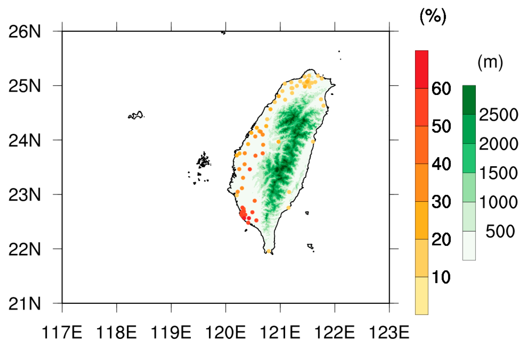
In this study, the hourly surface PM_2.5 concentration data observed at 73 Taiwan Environmental Protection Administration (EPA) ground stations from 2006 through 2015 were applied to identify the air pollution events. Following the definition of the Air Quality Index (AQI) from Taiwan EPA, we chose the criterion of “unhealthy” as the threshold of severe air pollution events, which corresponds to the 24-h averaged PM_2.5 concentrations above 54.5 µg m⁻³. [26,28] The location of the stations and the frequency of severe air pollution is shown in Figure 1. Most of the Taiwan EPA ground stations are located in the densely populated western plain areas. Among all the stations, the stations located in southwestern Taiwan are subject to severe air pollution conditions, the averaged PM_2.5 concentrations exceeding the threshold on more than 60% of the days over 2006–2015. The frequency of severe air pollution occurrence decreases from south to north, with 30–40% around central–western Taiwan and less than 20% in northern Taiwan. Contrasting to western Taiwan, there are only six stations to the east of CMR, and the frequencies of severe air pollution events are less than 10% due to the sparse population and lack of local emission.

To establish the relationship between synoptic weather condition and the severe PM_2.5 pollution events covering the Taiwan island, we established the Air Pollution Index (API) that considers the spatial extent of air both pollution events and is defined by the following steps. (1) The original time series of the PM_2.5 concentrations in each station is smoothed with a 24-h moving window to remove the high-frequency variations such as diurnal cycle or episodic agricultural burning events. (2) In the smoothed hourly time series, the number of stations with PM_2.5 concentrations surpassing 54.5 µg m⁻³ (i.e., unhealthy AQI condition) [28] are counted. (3) The ratio (in percentage) of the hourly station counts to the total number of Taiwan EPA stations (N_T = 73) is defined as the API,

$$API\left(t\right) = \frac{\mathrm{N}\left(\mathrm{t}\right)}{N_T}\times 100\%$$

(1)

$$\mathrm{N}\left(\mathrm{t}\right):{\mathrm{the}\mathrm{number}\mathrm{of}\mathrm{stations}\mathrm{PM}}_{2.5}>54.5{\mathrm{\mu }\mathrm{gm}}^{-3}\mathrm{at}\mathrm{time}\left(\mathrm{t}\right)$$

$$N_T:\mathrm{the}\mathrm{total}\mathrm{number}\mathrm{of}\mathrm{Taiwan}\mathrm{EPA}\mathrm{stations}.$$

The higher API represents a broader area influenced by severe PM_2.5 pollution. Many previous studies [20,21] have indicated that the meteorological information within a span is essential for the evolution of air pollution events. In this study, we focus on the API variation within the 240-h (i.e., 10-day synoptic time-scale) running window and investigate their relationship with the evolution of the synoptic weather.

Then, the time-series of API over a 240-h running window are processed through the machine learning method of hierarchical clustering. Hierarchical clustering analysis (HCA) is an unsupervised algorithm that groups data points with similar characteristics into clusters. In our study, the hierarchical clustering was conducted following the agglomerative strategy, which is also called a bottom–up approach [29]. At first, each 240-h segment of API data was treated as an individual sample, and new clusters formed by joining two elements with the closest Euclidean distance until the most significant final group was produced. We used Ward’s method [30] to minimalize the variance of data for each cluster. To use this method usually creates more compact and even-sized clusters with fewer computations with other methods. There are several advantages in using HCA, including that the number of clusters is not required for the algorithm, which is beneficial for understanding the data features. Figure S1 (Supplementary Materials) shows the final 20 clusters of HCA analysis. The top layer has two major air-pollution events: clean and dirty conditions. Dividing the events into only these two groups does not help us to explore the difference in atmospheric environmental conditions when air pollution events occur. In the second layer, the data are further divided into five groups (discussed in more detail in Section 3.1), two of which belong to events with a relatively clean atmosphere, while the other three categories represent conditions with more serious pollution, and they can be clearly distinguished from each other in the evolution of API time series. Therefore, with the consideration of both the classification significance and the common features within each cluster, we select these five clusters as final classification results.

To examine the weather conditions, we used 925 hPa horizontal wind fields from the ECMWF Reanalysis V5 (ERA5) hourly data at a horizontal resolution of 0.25° × 0.25° [31] to represent the lower atmospheric circulation. The Tropical Rainfall Measuring Mission (TRMM) 3B42 v7 precipitation data [32,33] and local vertical sounding (Taipei, WMO-46692) are used to show accumulated rainfall and atmospheric stability for various weather conditions. The daily synoptic weather event log acquired from the Taiwan Atmospheric event Database (TAD) [34] was also applied as an indicator of the synoptic weather conditions including cold surge (CS), frontal system (FT), northeasterly flow (NE), and strong northeasterly (SNE). If there is no major weather system listed above near Taiwan, we marked the day as a weak synoptic event (WS).

3. Results

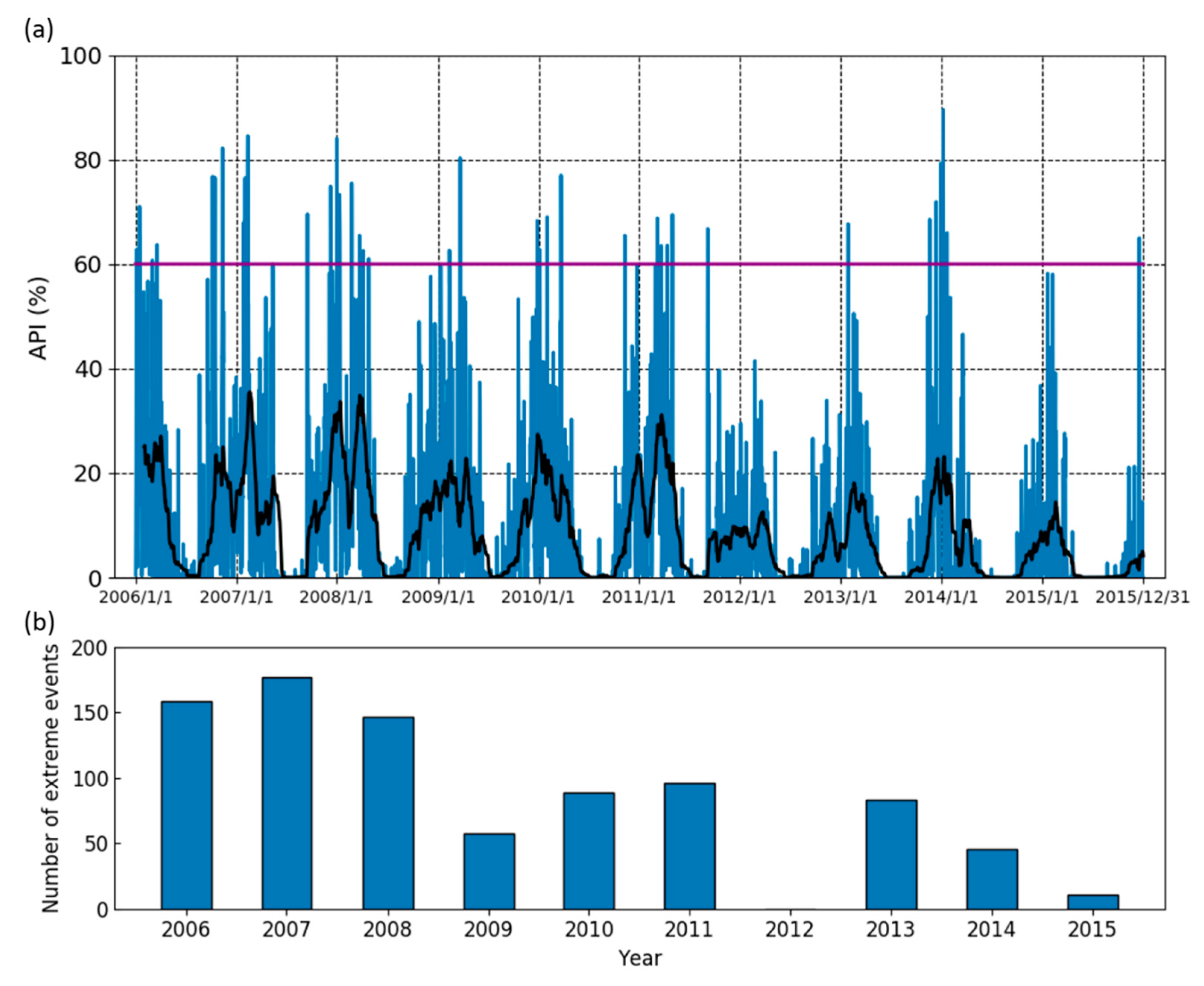
The time series of API from 2006 through 2015 is shown in Figure 2a. Most of the events with high API value occurred from October through March, which is when the northeasterly monsoonal flow prevails. The number of events with high API values and the average API were declining in recent years. We further examined the number of extreme events with the API values exceeding 60%, which is the threshold of the 99th percentile (top 1%) in the API data. As shown in Figure 2b, the frequency of extreme events decreased in recent years and varied on the inter-annual time scale.

3.1. Hierarchical Clustering

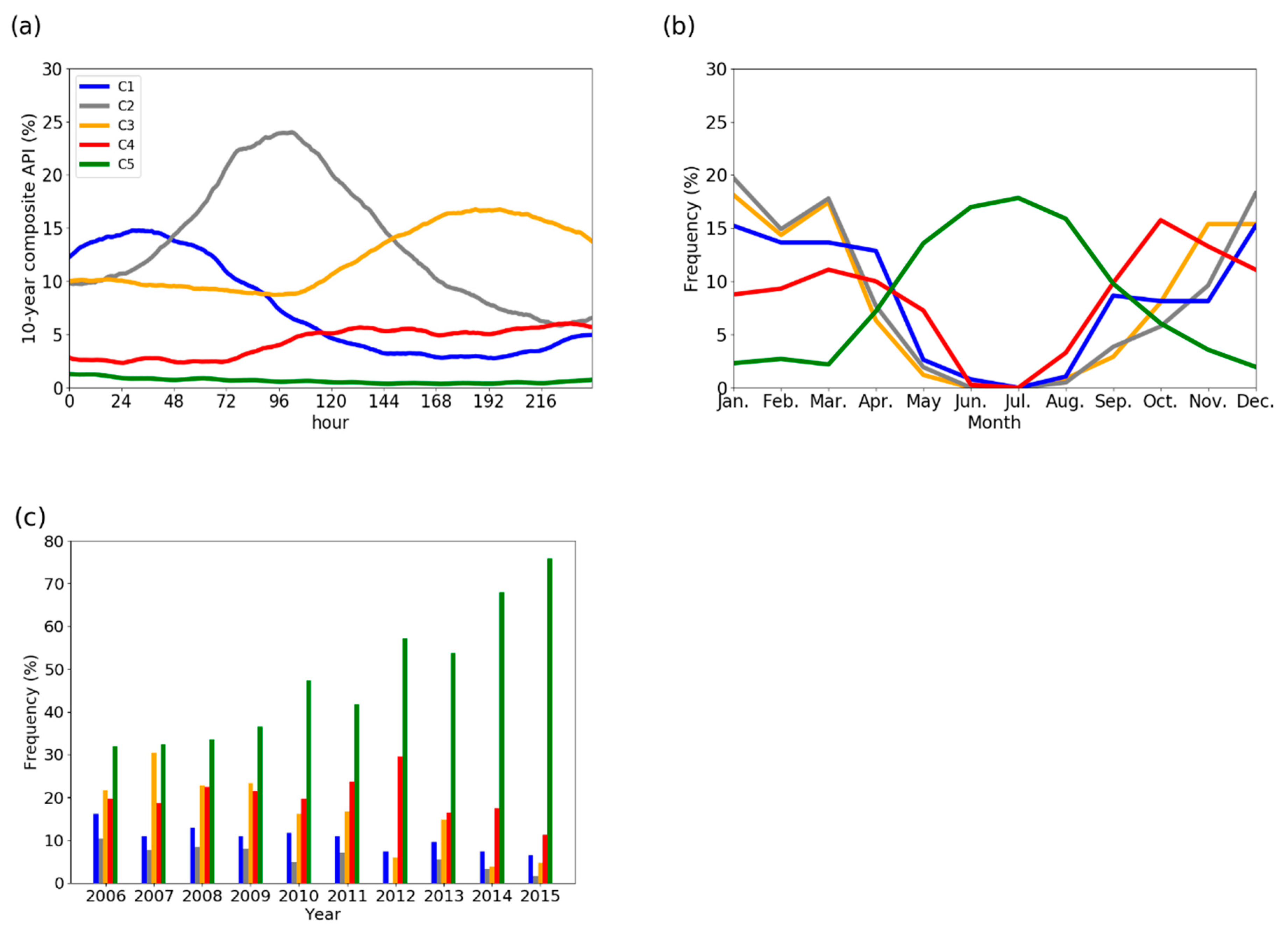
The composite API values of these five clusters over 2006–2015 are shown in Figure 3a; a distinct temporal evolution pattern characterizes each. In the 1st cluster (C1), API rises abruptly to above 15% in the earlier days of a 240-h window and declines rapidly, suggesting that most of the stations on the island exhibit severe air pollution, while the coverage of severe air pollution shrinks shortly after the peak. C2 is the most polluted cluster. The API rises rapidly within 72 h and reaches a peak value (25%) on the 4th day within a 240-h window, which indicates that the range of severe air pollution will expand to the entire island within four days and then decrease gradually. C3 contains multiple peaks in API values, and the air quality will be more polluted in the latter days of the 240-h window. C4 shows minor air pollution events in which only less than 8% of the stations are affected by severe air pollution but expands slightly in the latter days. C5 represents the cleanest condition, with the API values remaining lower than 5% for ten days.

The monthly occurrence frequencies of each cluster were also analyzed, as shown in Figure 3b. C1, C2, and C3 are associated with most severe pollution events and mainly occur from November through March. C4 distributes in winter (December–February), spring (March–Aprch), and autumn (September–November) months and is more frequent than C1–C3 in September and October. C5, the cleanest conditions, primarily occurs in summer. The occurrence frequency by year (Figure 3c) suggests that C1C3, the severely polluted conditions, were generally declining in 2006–2015, while C5 (clean condition) becomes more frequent; approximately 75 % of the events in 2015 were C5. The descending trend in the severe pollution clusters is consistent with the trend in the frequency of extreme events shown in Figure 2b.

To further establish the connection between the weather conditions and the air pollution events, the occurrence frequencies of the major synoptic weather types from TAD during October through March in 2006–2015 [34] were calculated for all days (Figure 4, white bars), and only for the days overlapped with the severe air pollution events (C1–C3). Su et al. [34] analyzed the monthly frequencies of the daily synoptic weather types in TAD. They reported that for each weather type, the frequency of occurrence can vary from month to month, but the relative composition of the different weather events is actually similar each month. Therefore, here, we use the frequency anomalies of air pollution types C1–C3 (colored bars in Figure 4) to better discern their relationships with the synoptic weather events. Higher frequency anomaly suggests that air pollution and weather events are more likely to occur concurrently. C1 and C2 clusters are more frequently associated with the weak synoptic weather condition and less likely with the NE and SNE. C3, on the contrary, occurs preferentially during NE, SNE, and FT. Note that the frequencies of C1–C3 under FT are close, since the changes in boundary layer conditions associated with FT are complicated. The wind speed and direction change significantly before and after the passage of the front, and the environmental condition would be WS-like if the wind speed decreases or NE-/SNE-like if the northeasterly wind enhances. The frontal precipitation can wash out the air pollutants. Among these weather events, CS is the rarest one, which is often accompanied by SNE. Hence, there is no further discussion on the air pollution events under CS.

We noticed that the evolution sequence and duration of the synoptic weather events could be different each month, leading to differences in the transition of air pollution clusters. In the following part, we selected two cases from winter and autumn, respectively, and closely examined the spatial and temporal pattern of API events and the corresponding weather conditions in more detail.

3.2. Case Study

3.2.1. Case Study: January 2006

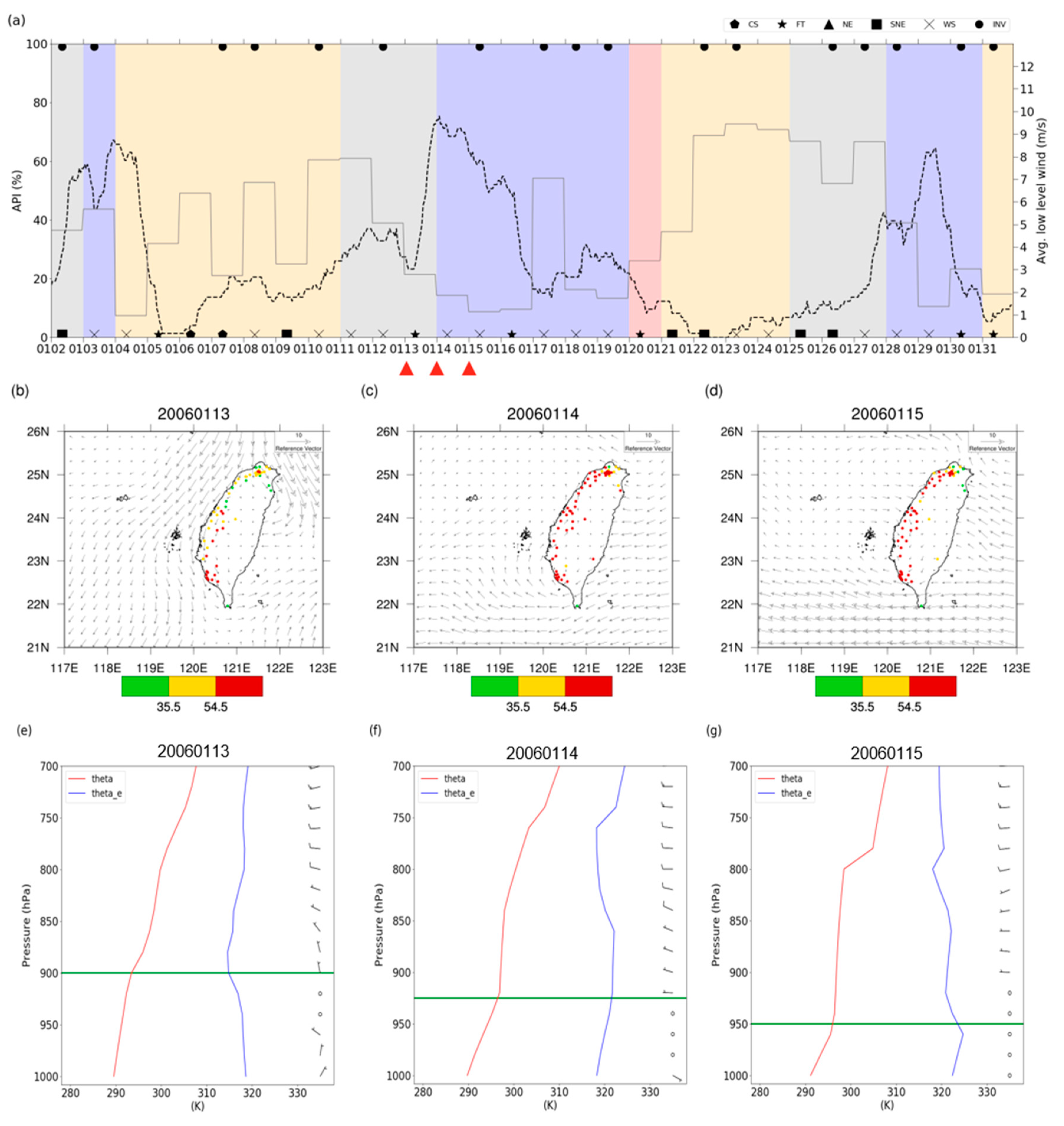
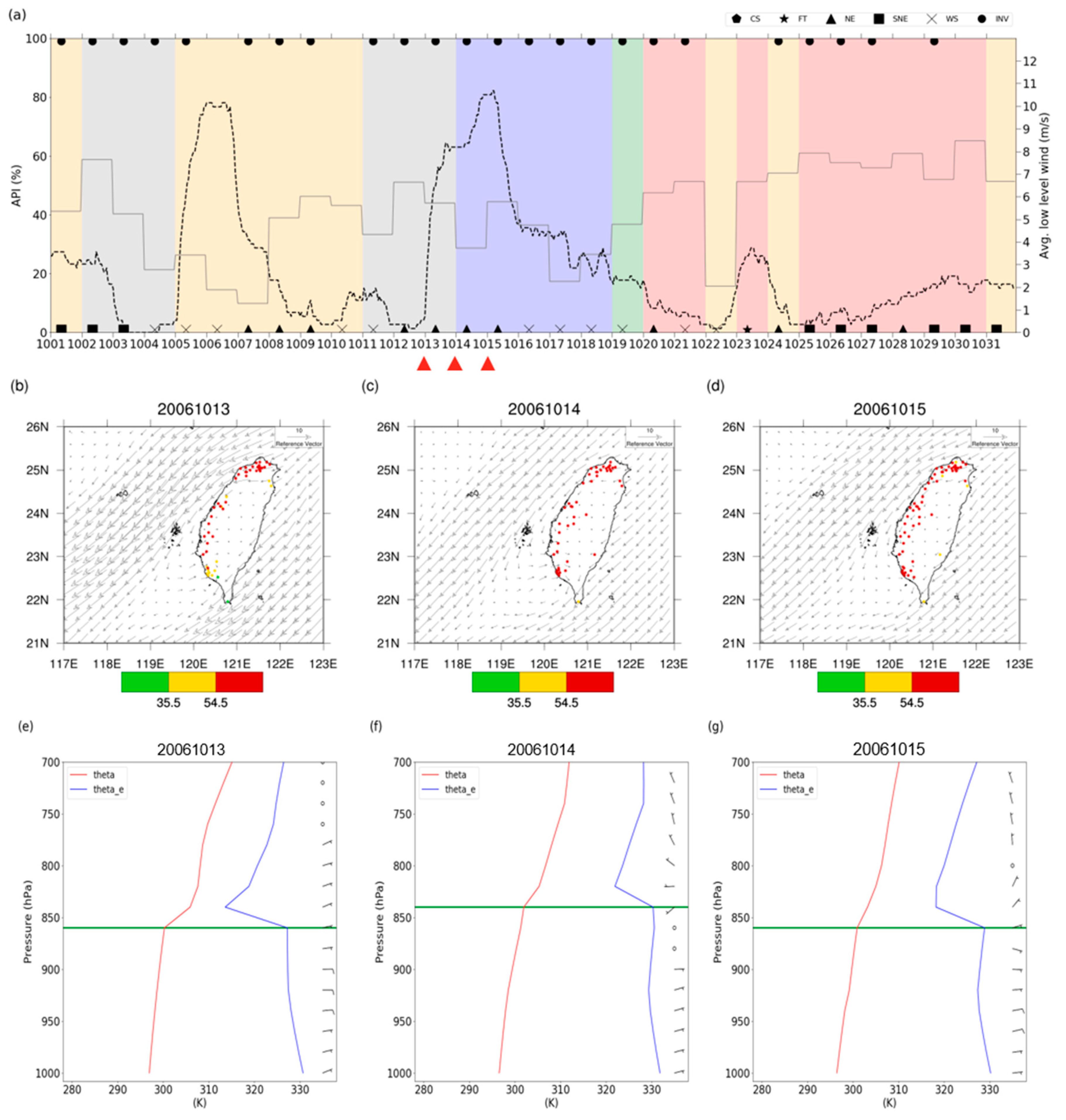
The API values, the beginning days of the clusters, and the corresponding weather conditions in January 2006 are shown in Figure 5a. There were three high API episodes on 2–4, 13–15, and 27–30 January. All three episodes were occurring during the days of persistent weak synoptic weather conditions. As the weak synoptic weather continued, the low wind speed near-surface favored the accumulation of air pollutants, and the temperature inversion in the low level hindered the vertical transport of air pollutants, which led to the rapid increase in API values. C1, C2, and C3 were the major clusters in this month; these clusters were transitioning between each other, which was attributable to the changing weather conditions. The beginning days of the three episodes (2nd, 13th, and 27th) were classified as C2, suggesting that API would peak (>60%) over five days during a spell of WS. C1 took over after days of C2, the days of C1 were characterized by a rapid rise and decline in API, and the decline was often associated with the occurrence of synoptic weather events. C3 occurred in the intermission of C2 and C1 when the persistent WS was interrupted by the synoptic weather events.

The wind field on 925 hPa and the distribution of the daily average PM_2.5 concentration on episode from 13 to 15 January 2006 is shown in Figure 5b–d. The passage of a weak front on the 13th was followed by two days of WS with low wind speed at the low level. As the wind speed decreased, the prevailing northeasterly wind turned easterly on 14th, and a lee-vortex circulation formed in southeastern Taiwan. On the 15th, there was a dipole of lee vortices over Taiwan Strait (Figure 5d). The lee circulation transported the air pollutants out of the land and back to the western plain, which further deteriorated the air quality. In addition, the temperature inversion layer capping the low level (Figure 5e–g), getting lower in the three days and also inhibiting the vertical transport of air pollutants, which helped to keep the air pollutants near the surface as well. The severely polluted condition was relieved as the frontal system passed through Taiwan on the 16th, which brought precipitation and strengthened the northeasterly wind.

3.2.2. Case Study: October 2006

In this month, there were two high API episodes in which the API ascended rapidly to 80% from the 5th to the 7th and the 13th to the 15th (Figure 6a). During the 13th–15th, the API rose in days of NE rather than continued WS and decreased after the 16th as the WS started. On 13th–15th, the low level was dominated by northeasterly winds, and the coverage of air pollutants was spreading from north to south since the sustained strong northeasterly winds served as a conveyor that transported air pollutants across a long distance from the East Asian continent (Figure 6b–d). There were some areas of rainfall on the sea in the three days (Figure S2 (Supplementary Materials)), and hence, the effect of rain scavenging on land was limited. Moreover, the capping inversion inhibited the vertical movement of the atmosphere, which was unfavorable to the vertical transport of air pollutants (Figure 6e–g). On the 16th–17th, the wind weakened and turned, the severely polluted area shrank to southwestern Taiwan where the wind speed is typically weak in the seasons when northeasterly prevails. The weather condition on the 5th–7th was characterized by northerly winds in the low level that transported the transboundary pollutants from north to south. The air quality improved as the wind direction changed and the wind speed strengthened.

Compared with January 2006, the air pollution events this month are associated with the influence of northerly or northeasterly winds and can result from the long-range transport (LRT) of air pollutants from the East Asian continent. The major clusters of the air pollution events in the earlier half of this month were C2 and C3. The episode during the 5th–7th was clustered into C3, since there was more than one peak in the 240-h windows including the two episodes resulting from LRT. C1 began on the 14th, indicating that there would be a decline in API value soon after the peak. It is worth noting that the API value was generally low after the 19th, which was attributable to the influence of the frequent synoptic weather events, including NE, SNE, and FT, contributing to the strong wind speed in the low level. The frequency of the synoptic weather events is determinant in the occurrence of PM_2.5 pollution events.

In addition to the sensitivity of the air pollution events to the synoptic weather events, we have also noticed that the transitions of the clusters showed different properties in the autumn and winter seasons. In winter, when the winter monsoonal circulation is established and the northeasterly is strong, the API tends to rise in the continuous days of WS, which is characterized by the weak northeasterly to southeasterly. Both the low wind speed and the lee-vortex formed on the lee-side of the CMR are favorable for the accumulation of air pollutants (Lai and Lin, 2020). In addition, the low level capped by the temperature inversion in winter also inhibits the vertical transport of air pollutants. However, in autumn, the season when the northeasterly monsoonal flow is establishing, the rapid increase in API values often arises from the long-range transport of the air pollutants on the days when northerly winds strengthen. The sequence of the synoptic weather systems can directly affect the distribution of air pollutants and further modulate the sequence of the clusters.

4. Discussion

Based on this research, we believe that the information of the synoptic weather evolutions has the potential to be a predictor of the time sequence of severe air pollution events. Currently, the meteorological forecast for PM_2.5 air pollution mainly relies on four different approaches. The first one relies on the empirical, statistical relationships among meteorological variables and concentrations of pollutants established using long-term station observations (e.g., [35]), reanalysis, and/or satellite data (e.g., [36]), such that the local air pollution events can be predicted by an optimized regression-based model using the single/multiple observations as input. The second approach uses the meteorological fields from numerical weather prediction to drive an offline chemical transport model or diffusion model to obtain the concentrations of specific pollutants (e.g., [37]). The third method, and the most computationally expensive one, is forecasting by the atmospheric model directly coupled to a detailed chemistry module (e.g., WRF-Chem) [38]. The advantage of using the interactive model can represent more realistic aerosol emission/transport/deposition over the simulated domain. However, the computational loading of this online model is much higher than the previous methods. Lastly, advanced statistical methods (artificial neural network/machine learning/deep learning) have been developed recently to predict PM_2.5 (e.g., [39,40,41]), which are based on the data-driven concept to generate the real-time or daily regional PM_2.5 predictions with relative efficiency. This study provides a foundation to understand the synoptic temporal evolution of the PM_2.5 pollution over Taiwan. In the future, one can use more advanced machine learning methods that can take the temporal dynamic behavior of synoptic weather information as input (e.g., recurrent neural network, RNN) to predict the temporal variation of the PM_2.5 concentrations. Then, we can take advantage of the numerical weather forecasting model, which generally has better performance on the evolution of synoptic weather patterns, to expand the predictable time-range for high PM_2.5 pollution events over the island.

5. Conclusions

In this study, we applied the hourly PM_2.5 concentration data observed at 73 Taiwan EPA ground stations from 2006 through 2015 to develop an air pollution indicator that depicts the overall state of air pollution within a spell over Taiwan island. The stations located in southwestern Taiwan were subject to severe air pollution events with a high frequency of more than 60%. Data samples with high API values are mainly distributed in October through March when the northeasterly monsoonal flow prevails. We focused on the API variation in all the 240-h time windows and grouped it via a hierarchical clustering algorithm. The top five clusters were identified. There are three clusters representing the major polluted events. C1 is characterized by an abrupt rise in API in earlier days of the 240-h time window followed by a decline, suggesting that most of the stations on the island were encountering severe air pollution, and the coverage of severe air pollution shrinks shortly. C2 is the most polluted cluster that shows a peak around the 4th–5th day in which the range of severe air pollution will expand to the entire island and then decrease gradually. C3 demonstrates multiple rises and falls in API in a 240-h time window, and the air quality will be more polluted in the latter days of the 240-h window. The clusters with the most severely polluted conditions are C1, C2, and C3, mainly occurring in autumn–winter–spring months when the northeasterly winds prevail. In addition, C1 and C2 are most likely to occur under weak synoptic weather conditions. In contrast, C3 is more frequently associated with the synoptic weather events of NE, SNE, and FT. The case studies from two selected months showed that the progression among the clusters is strongly affected by the sequence of the synoptic weather events, while the sequence of synoptic evolution exhibits different characteristics between the winter and autumn seasons.

To conclude, this study confirmed that the severe PM_2.5 pollution events could be uniquely classified by cluster analysis of a 10-day long time series. We also point out that in different clusters of high air pollution events, the transition of weather events will lead to changes in local circulation patterns and atmospheric stability, and it will also affect the time series evolution of air pollution events. These results all show that the evolution of the large-scale atmospheric conditions on the synoptic time scale (around 10 days) can become an essential basis for the diagnosis and the prediction of the air pollution events in Taiwan. In autumn, when the northeasterly monsoonal flow is transitioning, the rapid increase of pollutants often arises from the long-range transport of the air pollutants as the northerly winds are strengthening. In the winter season, when the East Asian winter monsoon is active and the low troposphere is stable, the sustained weak synoptic weather condition will lead to an abrupt increase in PM_2.5, while the severe air pollution can be relieved by the interruption of the synoptic weather events. In the future, the extended-range forecast of air pollution can potentially be conducted by constructing machine learning models to associate the sequence of synoptic weather patterns with specific pollution clusters identified in the present study.

References

- Hsu, C.H.; Cheng, F.Y. Synoptic weather patterns and associated air pollution in Taiwan. Aerosol Air Qual. Res. 2019, 19, 1139–1151. [Google Scholar] [CrossRef] [Green Version]
- Chuang, M.T.; Chou, C.C.K.; Lin, N.H.; Takami, A.; Hsiao, T.C.; Lin, T.H.; Fu, J.S.; Pani, S.K.; Lu, Y.R.; Yang, T.Y. A simulation study on PM2.5 source and meteorological characteristics at the northern tip of Taiwan in the early stage of the Asian haze period. Aerosol Air Qual. Res. 2017, 17, 3166–3178. [Google Scholar] [CrossRef] [Green Version]
- Chuang, M.T.; Lee, C.T.; Hsu, H.C. Quantifying PM2.5 from long-range transport and local pollution in Taiwan during winter monsoon: An efficient estimation method. J. Environ. Manag. 2018, 227, 10–22. [Google Scholar] [CrossRef]
- Cheng, F.Y.; Chin, S.C.; Liu, T.H. The role of boundary layer schemes in meteorological and air quality simulation of Taiwan area. Atmos. Environ. 2012, 54, 714–727. [Google Scholar] [CrossRef]
- Hsu, C.H.; Cheng, F.Y. Classification of weather patterns to study the influence of the meteorological characteristics on PM2.5 concentrations in Yunlin County, Taiwan. Atmos. Environ. 2016, 144, 397–408. [Google Scholar] [CrossRef]
- Miao, Y.; Liu, S.; Zheng, Y.; Wang, S.; Cheng, B.; Zheng, H.; Zhao, J. Numerical study of the effects of local atmospheric circulations on a pollution event over Beijing-Tianjin-Hebei, China. J. Environ. Sci. 2015, 30, 9–20. [Google Scholar] [CrossRef]
- Ding, A.; Huang, X.; Fu, C. Air pollution and weather interction in East Asia. Oxf. Res. Encycl. Environ. Sci. 2017, 1, 1–26. [Google Scholar] [CrossRef]
- Wu, C.H.; Tsai, I.C.; Tsai, P.C.; Tung, Y.S. Large-scale seasonal control of air quality in Taiwan. Atmos. Environ. 2019, 214, 116868. [Google Scholar] [CrossRef]
- Li, T.C.; Yuan, C.S.; Huang, H.C.; Lee, C.L.; Wu, S.P.; Tong, C. Inter-comparison of seasonal variation, chemical characteristics, and source identification of atmospheric fine particles on both sides of the Taiwan Strait. Sci. Rep. 2016, 6, 22956. [Google Scholar] [CrossRef] [Green Version]
- Chen, C.S.; Chen, Y.L. The rainfall characteristics of Taiwan. Mon. Wea. Rev. 2003, 131, 1323–1341. [Google Scholar] [CrossRef]
- Chang, C.P.; Lu, M.M.; Wang, B. The East Asian winter monsoon. In The Global Monsoon System: Research and Forecast, 2nd ed.; Chang, C.P., Ding, Y.H., Lau, N.C., Johnson, R.H., Wang, B., Yasunari, T., Eds.; World Scientific Publisher: Singapore, 2011; Volume 5, pp. 99–109. ISBN 978-981-4343-40-4. [Google Scholar]
- Chen, T.C.; Yen, M.C.; Wang, W.R.; Gallus, W.A., Jr. An East Asian cold surge: Case study. Mon. Weather Rev. 2002, 130, 2271–2290. [Google Scholar] [CrossRef]
- Chien, F.C.; Kuo, Y.H. Topographic effects on wintertime cold front in Taiwan. Mon. Weather Rev. 2006, 134, 3297–3316. [Google Scholar] [CrossRef] [Green Version]
- Gimson, N.R. Dispersion and removal of pollutants during the passage of an atmospheric frontal system. Q. J. R. Meteorol. Soc. 1994, 120, 139–160. [Google Scholar] [CrossRef]
- Chi, K.H.; Lin, C.Y.; Ou-Yang, C.F.; Wang, J.L.; Lin, N.H.; Sheu, G.R.; Lee, C.T. PCDD/F Measurement at a high-altitude station in central Taiwan: Evaluation of long-range transport of PCDD/Fs during the southeast Asia biomass burning event. Environ. Sci. Technol. 2010, 44, 2954–2960. [Google Scholar] [CrossRef]
- Sheu, G.R.; Lin, N.H.; Wang, J.L.; Lee, C.T.; Ou-Yang, C.F.; Wang, S.H. Temporal distribution and potential sources of atmospheric mercury measured at a high-elevation background station in Taiwan. Atmos. Environ. 2010, 44, 2293–2400. [Google Scholar] [CrossRef]
- Lee, C.T.; Chuang, M.T.; Lin, N.H.; Wang, J.L.; Sheu, G.R.; Chang, S.C.; Wang, S.H.; Huang, H.; Chen, H.W.; Liu, Y.L.; et al. The enhancement of PM2.5 mass and water-soluble ions of biosmoke transported from Southeast Asia over the Mountain Lulin site in Taiwan. Atmos. Environ. 2011, 45, 5784–5794. [Google Scholar] [CrossRef]
- Hsiao, T.C.; Chen, W.N.; Ye, W.C.; Lin, N.H.; Tsay, S.C.; Lin, T.H.; Lee, C.T.; Chuang, M.T.; Pantina, P.; Wang, S.H. Aerosol optical properties at the Lulin Atmospheric Background Station in Taiwan and the influences of long-range transport of air pollutants. Atmos. Environ. 2017, 150, 366–378. [Google Scholar] [CrossRef]
- Gangoiti, G.; Millán, M.M.; Salvador, R.; Mantilla, E. Long-range transport and re-circulation of pollutants in the western Mediterranean during the project Regional Cycles of Air Pollution in the West-Central Mediterranean Area. Atmos. Environ. 2001, 35, 6267–6276. [Google Scholar] [CrossRef]
- Fiddes, S.L.; Pezza, A.B.; Mitchell, T.A.; Kozyniak, K.; Mills, D. Synoptic weather evolution and climate drivers associated with winter air pollution in New Zealand. Atmos. Pollut. Res. 2016, 7, 1082–1089. [Google Scholar] [CrossRef] [Green Version]
- Ferenczi, Z. Predictability analysis of the PM2.5 and PM10 concentration in Budapest. Időjárás 2013, 117, 359–375. [Google Scholar]
- Lai, H.C.; Lin, M.C. Characteristics of the upstream flow patterns during PM2.5 pollution events over a complex island topography. Atmos. Environ. 2020, 227, 117418. [Google Scholar] [CrossRef]
- Smith, R.B.; Grubišić, V. Aerial observations of Hawaii’s wake. J. Atmos. Sci. 1993, 50, 3728–3750. [Google Scholar] [CrossRef] [Green Version]
- Lesouëf, D.; Gheusi, F.; Delmas, R.; Escobar, J. Numerical simulations of local circulations and pollution transport over Reunion Island. Ann. Geophys. 2011, 29, 53–69. [Google Scholar] [CrossRef] [Green Version]
- Yang, Y.; Chen, Y.L. Effects of terrain heights and sizes on island-scale circulations and rainfall for the island of Hawaii during HaRP. Mon. Weather Rev. 2008, 136, 120–146. [Google Scholar] [CrossRef] [Green Version]
- Cheng, F.Y.; Hsu, C.H. Long-term variations in PM2.5 concentrations under changing meteorological conditions in Taiwan. Sci. Rep. 2019, 9, 6635. [Google Scholar] [CrossRef]
- Alpert, P.; Osetinsky, I.; Ziv, B.; Shafir, H. A new seasons definition based on classified daily synoptic systems: An example for the eastern Mediterranean. Int. J. Climatol. 2004, 24, 1013–1021. [Google Scholar] [CrossRef]
- Environmental Protection Administration, Executive Yuan, Taiwan. Documentary on Air Quality Protection. Available online: https://www.epa.gov.tw/eng/5FF11AF44EF9533B (accessed on 1 May 2020).
- Hexmoor, H. Diffusion and Contagion-Hierarchical Clustering. In Computational Network Science: An Algorithm Approach; Hexmoor, H., Ed.; Morgan Kaufmann: San Mateo, CA, USA, 2015; pp. 45–64. ISBN 978-0-12-800891-1. [Google Scholar]
- Ward, J.H., Jr. Hierarchical Grouping to Optimize an Objective Function. J. Am. Stat. Assoc. 1963, 58, 236–244. [Google Scholar] [CrossRef]
- Hersbach, H.; Dee, D. ERA5 Reanalysis Is in Production. ECMWF Newsletter. Available online: https://www.ecmwf.int/en/newsletter/147/news/era5-reanalysis-production (accessed on 1 May 2020).
- Kummerow, C.; Simpson, J.; Thiele, O.; Barnes, W.; Chang, A.T.C.; Stocker, E.; Adler, R.F.; Hou, A.; Kakar, R.; Wentz, F.; et al. The Status of the Tropical Rainfall Measuring Mission (TRMM) after Two Years in Orbit. J. Appl. Meteorol. 2000, 39, 1965–1982. [Google Scholar] [CrossRef]
- Huffman, G.J.; Adler, R.F.; Bolvin, D.T.; Nelkin, E.J. The TRMM Multi-Satellite Precipitation Analysis (TMPA). In Satellite Rainfall Applications for Surface Hydrology; Gebremichael, M., Hossain, F., Eds.; Springer: Dordrecht, The Netherlands, 2010; pp. 3–22. ISBN 978-90-481-2915-7. [Google Scholar]
- Su, S.H.; Chu, J.L.; Yo, T.S.; Lin, L.Y. Identification of synoptic weather types over Taiwan area with multiple classifiers. Atmos. Sci. Lett. 2018, 19, e861. [Google Scholar] [CrossRef] [Green Version]
- Li, J.; Li, X.; Wang, K. Atmospheric PM2.5 Concentration Prediction Based on Time Series and Interactive Multiple Model Approach. Adv. Meteorol. 2019. [Google Scholar] [CrossRef] [Green Version]
- Lin, C.A.; Chen, Y.C.; Liu, C.Y.; Chen, W.T.; Seinfeld, J.H.; Chou, C.C.K. Satellite-Derived Correlation of SO2, NO2, and Aerosol Optical Depth with Meteorological Conditions over East Asia from 2005 to 2015. Remote Sens. 2019, 11, 1738. [Google Scholar] [CrossRef] [Green Version]
- Brandt, J.; Silver, J.D.; Frohn, L.M.; Geels, C.; Gross, A.; Hansen, A.B.; Hansen, K.M.; Hedegaard, G.B.; Skjøth, C.A.; Villadsen, H.; et al. An integrated model study for Europe and North America using the Danish Eulerian Hemispheric Model with focus on intercontinental transport of air pollution. Atmos. Environ. 2012, 53, 156–176. [Google Scholar] [CrossRef]
- Grell, G.A.; Peckham, S.E.; Schmitz, R.; McKeen, S.A.; Frost, G.; Skamarock, W.C.; Eder, B. Fully coupled ’online’ chemistry in the WRF model. Atmos. Environ. 2005, 39, 6957–6976. [Google Scholar] [CrossRef]
- Le, V.D.; Cha, S.K. Real-time air pollution prediction model based on spatiotemporal big data. Presented at the International Conference on Big data, IoT, and Cloud Computing (BIC 2018), Jeju, Korea, 20–22 August 2018. [Google Scholar]
- Maleki, H.; Sorooshian, A.; Goudarzi, G.; Baboli, Z.; Birgani, Y.T.; Rahmati, M. Air pollution prediction by using an artificial neural network model. Clean Technol. Environ. Policy 2019, 21, 1341–1352. [Google Scholar] [CrossRef]
- Pak, U.; Ma, J.; Ryu, U.; Ryom, K.; Juhyok, U.; Pak, K.; Pak, C. Deep learning-based PM2.5 prediction considering the spatiotemporal correlations: A case study of Beijing, China. Sci. Total Environ. 2020, 699, 133561. [Google Scholar] [CrossRef]
Figure 1.
The terrain height distribution over Taiwan (green shadings) and locations of the Taiwan Environmental Protection Administration (EPA) air-quality stations (colored dots, with the red shading representing the climatological frequency of occurrence of severe air pollution events (fine particulate matter (PM2.5) >54.5 μg m−3) over 2006–2015 (unit: %) in each station.
Figure 2.
(a) Air Pollution Index (API) from 2006 through 2015 is represented by the blue line. The black line shows the one-smooth running average of API, and the horizontal purple line is the 60% threshold value to define extreme events. (b) The number of extreme events (API > 60%, 99 percentile) from 2006 to 2015 is represented by the blue bars.
Figure 3.
(a) Composite API values over 2006 to 2015 of each cluster, (b) Monthly frequency of occurrence of each cluster. (c) Annual frequency of each cluster over 2006–2015. The blue, gray, orange, red, and green lines represent cluster 1, cluster 2, cluster 3, cluster 4, and cluster 5, respectively.
Figure 4.
Climatological frequencies of the synoptic weather events (white bars) and the frequency anomaly of the weather events in C1–C3 (colored bars) from October to March in 2006–2015 based on Taiwan Atmospheric event Database. Here, the frequency anomaly of the weather events is defined as the difference between the climatological frequency of the weather events and the frequency that a certain cluster occurred concurrently with the weather events.
Figure 5.
The case study for January 2006. (a) API time series (dashed line), the low-level wind speed averaged over the surface to 925 hPa (thin line), the near-surface temperature inversion around boundary layer top (black dot), and weather event (black symbols) in this month. The shadings in the background represent the beginning day of the air pollution clusters (blue for C1, gray for C2, yellow for C3, and pink for C4). The red triangles on the x-axis mark the High API episode through the 13th to the 15th. (b–d) are the daily mean PM2.5 concentrations (color dots; units: μg m−3) and wind field on 925 hPa (vectors; unit: m s−1) from the 13th to 15th. (e–g) are the vertical profiles of potential temperature (red line), the equivalent potential temperature (blue line), and wind (arrows) at Taipei (WMO-46692) from the 13th to 15th. The green line represents the level of temperature inversion.
Figure 6.
The case study for October 2006. (a) API time series (dashed line), the low-level wind speed averaged over the surface to 925 hPa (thin line), the near-surface temperature inversion around boundary layer top (black dot), and weather event (black symbols) in this month. The shadings in the background represent the beginning day of the air pollution clusters (blue for C1, gray for C2, yellow for C3, and pink for C4). The red triangles on the x-axis mark the High API episode through the 13th to the 15th. (b–d) are the daily mean PM2.5 concentrations (color dots; units: μg m−3) and wind field on 925 hPa (vectors; unit: m s−1) from the 13th to 15th. (e–g) are the vertical profiles of potential temperature (red line), the equivalent potential temperature (blue line), and wind (arrows) at Taipei (WMO-46692) from the 13th to 15th. The green line represents the level of temperature inversion.
Publisher’s Note: MDPI stays neutral with regard to jurisdictional claims in published maps and institutional affiliations. |
© 2020 by the authors. Licensee MDPI, Basel, Switzerland. This article is an open access article distributed under the terms and conditions of the Creative Commons Attribution (CC BY) license (http://creativecommons.org/licenses/by/4.0/).
Share and Cite
MDPI and ACS Style
Su, S.-H.; Chang, C.-W.; Chen, W.-T. The Temporal Evolution of PM2.5 Pollution Events in Taiwan: Clustering and the Association with Synoptic Weather. Atmosphere 2020, 11, 1265. https://doi.org/10.3390/atmos11111265
AMA Style
Su S-H, Chang C-W, Chen W-T. The Temporal Evolution of PM2.5 Pollution Events in Taiwan: Clustering and the Association with Synoptic Weather. Atmosphere. 2020; 11(11):1265. https://doi.org/10.3390/atmos11111265
Chicago/Turabian StyleSu, Shih-Hao, Chiao-Wei Chang, and Wei-Ting Chen. 2020. "The Temporal Evolution of PM2.5 Pollution Events in Taiwan: Clustering and the Association with Synoptic Weather" Atmosphere 11, no. 11: 1265. https://doi.org/10.3390/atmos11111265
Note that from the first issue of 2016, this journal uses article numbers instead of page numbers. See further details here.