Article

Skill of Mesoscale Models in Forecasting Springtime Macrophysical Cloud Properties at the Savannah River Site in the Southeastern US

Savannah River National Laboratory, Aiken, SC 29808, USA
*
Author to whom correspondence should be addressed.
Atmosphere 2020, 11(11), 1202; https://doi.org/10.3390/atmos11111202
Submission received: 30 September 2020 / Revised: 3 November 2020 / Accepted: 3 November 2020 / Published: 6 November 2020
(This article belongs to the Section Meteorology)

Abstract

:
Predicting boundary layer clouds is important for the accurate modeling of pollutant dispersion. Higher resolution mesoscale models would be expected to produce better forecasts of cloud properties that affect dispersion. Using ceilometer observations, we assess the skill of two operational mesoscale models (RAMS and WRF) to forecast cloud base altitude and cloud fraction at the Savannah River Site in the southeastern US during the springtime. Verifications were performed at small spatial and temporal scales necessary for dispersion modeling. Both models were unreliable with a 50% (RAMS) and a 46% (WRF) rate of predicting clouds observed by the ceilometer which led to low cloud fraction predictions. Results indicated that WRF better predicted daytime cloud bases from convection that occurred frequently later in the period and RAMS better predicted nighttime cloud bases. Using root mean squared error (RMSE) to score the forecast periods also highlighted this diurnal dichotomy, with WRF scores better during the day and RAMS scores better at night. Analysis of forecast errors revealed divergent model cloud base biases—WRF low and RAMS high. A hybrid solution which weighs more heavily the RAMS nighttime forecasts and WRF daytime forecasts will likely provide the best prediction of cloud properties for dispersion.

1. Introduction

Scavenging and absorption of atmospheric particles and gases by boundary layer clouds affect the dispersion of pollutants. The processes of washout, chemical transformations, and sedimentation upon droplet evaporation of constituents all impact the rate of atmospheric removal or deposition. To predict the interactions between atmospheric aerosols and cloud droplets, models need to accurately predict clouds within the boundary layer. Large spatial or temporal variability in cloud field predictions will lead to incorrect localization of clouds that fail to correctly interact with the plume limiting dispersion predictions on small scales.
The variable scale nature of clouds and cloud processes make them difficult to model. Small- scale interactions within clouds require state of the art microphysical and cumulus parameterizations [1] to estimate cloud properties for most mesoscale to global-scale meteorological simulations. Correctly parameterizing cloud processes is complicated by feedbacks by which clouds modify their own environment. For example, the formation of clouds modifies the local environment by moderating Earth’s energy balance and releasing latent heat to the atmosphere [2,3,4].
In dispersion modeling, clouds and precipitation drive wet deposition. Transformations of atmospheric aerosols and chemical constituents occur in clouds which, upon evaporation, leave altered aerosols [5] and modify airborne concentrations. Additionally, clouds moderate photochemistry affecting these constituents [6]. These interactions highlight the importance of accurate cloud forecasts. Recent emphasis on high frequency solar forecasting to manage electricity loads further demonstrates the important role of cloud prediction [7]. Understanding and improving cloud modeling aids to improve functionality for these types of forecasts.
Studies that assess cloud forecasts are primarily performed for cloud cover (cloud fraction) and cloud ceiling (base) height necessary for aviation safety [8,9,10,11,12]. Other studies focus on validating cloud properties from cloud parameterizations for use in large scale climate models [13]. Most of these studies use models with grid spacing greater than 6 km. Fewer have used higher resolution models (<2 km) in these assessments [7,14], but note that higher resolution models performed better at resolving the lower boundary layer cloud base heights (<500 m) that might affect dispersion.
The Savannah River National Laboratory utilizes two operational mesoscale models, the Regional Atmospheric Modeling System [15] (RAMS) and the Weather Research and Forecasting model [16] (WRF), to produce forecasts for the Savannah River Site (SRS) located in western South Carolina along the Savannah River near Aiken, SC (Figure 1). These forecasts support a variety of site operations including identifying weather patterns which can impact site operations, assisting the prescribed burns conducted by the US Forest Service at SRS and driving site dispersion modeling for emergency response. Verification studies of the models used for dispersion purposes [17] provide confidence in constituent fate and transport predictions.
Observational data sets that have previously been used to perform cloud forecast assessments include satellite data (cloud fraction/mask and brightness temperatures) [8,13], cloud radar and lidar networks [9,11,18], observation networks [14], pyranometer networks [7], and radiosondes [12]. Techniques for verifying cloud forecasts using satellite data include global analysis to compare with 3 h global models [8] and grid point or area comparisons [7,13,19]. Verification techniques using observation networks include area averaging [11,14] and probabilistic comparisons [18]. Radiosonde relative humidity profiles were also used to verify model cloud base height [12].
In this study, we provide an assessment of model capabilities in forecasting cloud macrophysical properties that affect atmospheric constituent dispersion at fine spatial and temporal scales. We use 15-min averaged ceilometer data at SRS to compare with 15-min WRF and RAMS forecast output of cloud properties. Comparisons between single point temporal measurements and instantaneous spatial measurements are highly dependent on resolution and advection [14]. For high-quality dispersion modeling, model resolution becomes very important. Horizontal grid spacings used in this assessment are 1.3 km for WRF and 1 km for RAMS. We use a spatial averaging method based on cloud field advection by the model wind speed to compare model forecasts every 15 min to 15-min averaged ceilometer cloud fraction and cloud base height. Synoptic conditions during the springtime in the southeastern US can be quite variable. Cloud formation can be driven by forcing from local diabatic heating, large-scale low-pressure systems and frontal passages, and sea breeze penetration among others. Clouds range from low level stratus and fog to deep convective thunderstorms. Therefore, the time period from April to June provides a robust evaluation of these two models.

2. Methods

To facilitate comparisons in this study, data are taken from both RAMS and WRF runs that were initiated at 18:00 UTC using the 18:00 UTC forecast of the 12 km North American Mesoscale Forecast System (NAM), available through the National Centers for Environmental Prediction [20]. The first six hours of simulations were used to spin up the model and assessments for this study began with the forecast period at 00:00 UTC. RAMS simulations were for 42 h and WRF simulations were for 36 h, producing 36 h RAMS forecasts and 30 h WRF forecasts. Both models generate gridded forecasts every 15 min. These model configurations have been tuned over the years to provide the best regional meteorological forecasts for key variables which affect atmospheric dispersion processes: temperature, humidity, wind speed, and wind direction.

2.1. RAMS

The RAMS model (v6.2.06) [21] was configured with two domains; a 600 × 500 km outer domain with 5 km horizontal grid spacing and 102 × 92 km nested domain (Figure 1) with 1 km grid spacing. Both domains were centered on the Savannah River Site and have 37 vertical grid boxes with the lowest grid spacing 25 m deep and the highest 1000 m. Intermediate levels are stretched by a factor of 1.2 until reaching 1000 m. Five model soil levels are used at 2.5, 15, 30, 50 and 70 cm below the surface. Soil moisture initialization uses a constant saturation fraction of 0.29. Soil temperature is initialized by the offset in temperature between three measured soil temperature levels (1, 6 and 12 inches) and the two-meter temperature measurement from the relative humidity probe at the SRS Climatology Site. Temperature offsets for the lowest two soil levels are estimated by calculating the slope of the 6- and 12-inch measurements and dividing by 2, for the 50 cm level, or 4, for the 70 cm level. This creates a more realistic soil temperature profile for model initialization. Additional information for topography, soil, and vegetation are read in from standard RAMS data files with a 30 arc second resolution.
Following the guidelines of the model developers [22], no cumulus parameterizations were used for either grid. Traditional convective parameterizations have been shown to overpredict precipitation and initiate convection too early in the southeastern United States [23]. The operational RAMS model utilizes the Harrington two-stream radiation parameterization [24] updated every 1200 s, and the Mellor and Yamada [25] diffusion parameterization scheme. The minimum value for the horizontal diffusion coefficient was set to 0.9 for the outer grid and 0.7 is used for the inner nested grid. The operational RAMS model utilizes the two-moment bin emulating bulk microphysical parameterization [26,27] with aerosol regeneration and wet and dry deposition activated. The ice nucleation scheme uses the Demott 2010 composite aerosol ice nuclei formula [28]. Cloud condensation nuclei are initialized with a concentration of 500 mg−1 and diameter of 100 nm and 120 nm when regenerated with typical solubility fractions.
During the time period 31 March to 30 June (2020), only one of the RAMS operational runs failed (missing data for 22 April). The failure was due to aerosols exceeding the maximum values close to steep terrain near grid outer grid boundary.

2.2. WRF

The operational WRF (v3.81) [29] model was configured with two domains; 400 × 400 km outer domain with 4 km horizontal grid spacing and nested domain about 89 × 89 km (Figure 1) with a grid spacing of 1.33 km. Both domains surrounded the Savannah River Site and have 35 vertical levels. The model uses four soil levels and soil initialization is provided by the operational North American Mesoscale (NAM) [30] forecast model grids. Information for soil type and vegetation [31] is provided by the NLCD2011 database. Topography for the large domain is 30 arc second and 1 arc second for the inner domain. Assimilation of temperature, moisture and wind information from the SRS meteorological towers is used operationally, with observations available at a 15-min frequency for the first 2 h of model integration.
The Thompson microphysical parameterization [32], which includes double moment parameters for rain and ice but not for cloud, was used for the WRF operational model. This operational model used the improved Grell 3D cumulus parameterization [33] that can be used on higher resolution domains. The radiation parameterization uses an improved Rapid Radiative Transfer Model (RRTMG) scheme [34] and the boundary layer parameterization uses the Mellor–Yamada–Janjic scheme [35].
Cloud data collection from WRF runs began on 2 April, so data are missing for 1 April. WRF cloud data are also missing for 19 April and 28 June because the 18 UTC runs failed on those days.

2.3. Cloud Base Altitude and Cloud Fractions

At SRS, a Vaisala CL31 ceilometer [36] measured cloud base altitude (CBA), when present, every 15 s. These were used to calculate a 15-min averaged CBA and a 15-min cloud fraction (CF). CF was calculated based on the fraction of time that a cloud base was detected during that period. The averaging was performed to center the 15-min periods on the quarter hours to provide the nearest representation to the 15-min model forecast times. For additional analysis, daily averaged CBA and CF were also calculated. On two separate days the ceilometer data were unavailable for short periods of 3.25 (18 April) and 2.5 h (27 June).
CBA and CF for the models were determined by examining the cloud properties in the grid cells in the proximity of the ceilometer. The specific grid cells were selected using model horizontal wind components (U and V) at the location of the ceilometer. The U and V components were taken from the model level nearest 2 km above the surface (median climatological daily CBA at SRS). Calculations from U and V (m/s) determined the distance (km) traveled in 15-min of a possible cloud field in the west–east (U) and south–north (V) directions. These values were used as an estimate to cloud advection and therefore select the number of grid boxes within a rectangle centered on the ceilometer to be used for CBA and CF calculations. The rectangle sizing and centering were performed to better match the ceilometer averaging mentioned previously. To increase statistics in cases with low wind speeds, an extra grid box is added in each direction. The lowest level of the vertical grid with a cloud water mixing ratio of at least 0.01 g/kg [37] or an ice water mixing ratio of at least 0.003 g/kg [38,39] is determined for each horizontal grid box within the rectangle. These limits are imposed as a better comparison for the clouds measured by the ceilometer. Model CBA used for comparisons is the average CBA of all the grid cells within the rectangle and model CF is the fraction of grid cells that have a valid CBA within that same rectangle. While this method differs from other commonly used methods for determining these values, it allows for the comparison of the instantaneous model spatial forecast data with the time averaged ceilometer cloud properties focused on a specific location rather than over a region covered by satellite or multiple cloud-measurement sites where the focus is on identifying whether the model produced the observed behavior within a reasonable vicinity of the measurement. For this application, we are more concerned with whether the modeled clouds occurred at the same location and time as the measurement as would be necessary for dispersion calculations. Only the nested domains were used for this analysis.

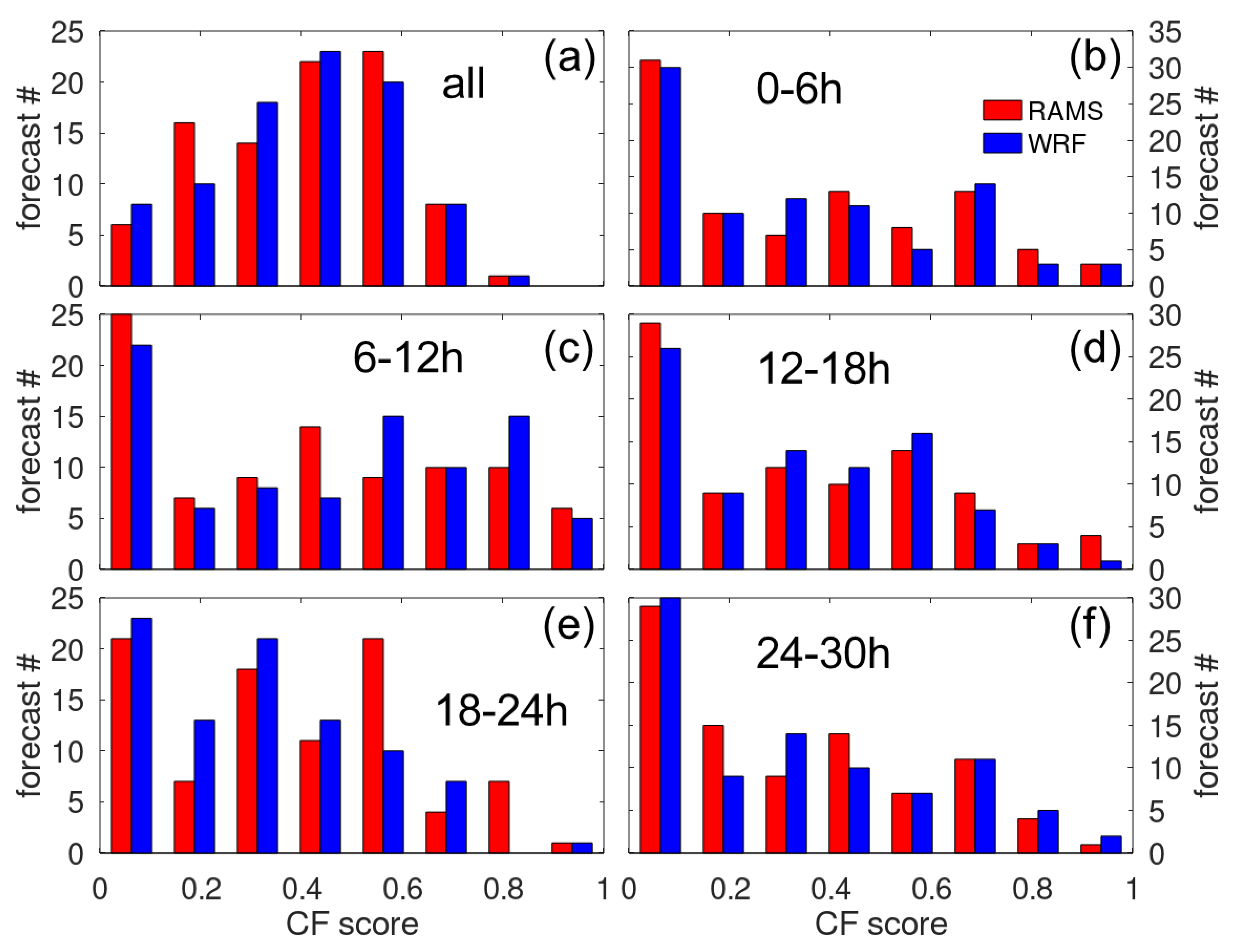
2.4. Cloud Forecast Scoring

Root mean squared error (RMSE) was used to score models on their ability to closely forecast CBA and CF. For CF, this was a simple process of taking the square root of the mean of the squared difference between the model value (predicted) and the ceilometer value (observed) for all 15-min values in a daily forecast. CBA scores were more complicated. Clouds near the surface within the boundary layer are most likely to affect dispersion. Thus, we set a maximum error limit of 2500 m because any cloud base error beyond that would likely be irrelevant to the dispersion. Additionally, we use the same maximum error for cases when models failed to develop cloud when observed by the ceilometer or created clouds when absent in ceilometer observations. All CBA scores were then normalized by a value of 2500; this allows us to quickly identify all cases when there was a discrepancy between the ceilometer and the models regarding whether clouds had formed because these cases will all be scored as a 1.0. After normalizing, the RMSE for CBA follows the process for CF. Because we use RMSE, lower scores indicate better forecasts (less error). Only the 15-min forecast times for the 30 h forecasts were used in scoring to provide a fair scoring comparison between RAMS and WRF. Besides scoring each 30 h forecast, each forecast was also divided into five 6 h periods and scored.

3. Results and Discussion

3.1. Fifteen-Minute Monthly Averaged Forecasts

Forecasts and observations are averaged monthly for each 15-min forecast time and corresponding observation time. Monthly ceilometer CF averages showed the least cloud in April (0.28) and increasing in May (0.30) and June (0.34) which is opposite the climatological trend where monthly CF decreases from April to June. The fewer clouds (smaller sample size) in April could be what leads to the apparent variability in ceilometer CBA in Figure 2a that the models have difficulty in forecasting. Additionally, clouds in April are more likely to be driven by synoptic scale events compared to May and June where local convection is more prominent. One such example was a widespread tornado outbreak in South Carolina from a frontal passage on 13 April 2020. Thus, deviations in both RAMS and WRF CBA compared to the ceilometer CBA (Figure 2a) could also be due to issues with timing of these synoptic scale events by the models.
Differences in the accuracy of cloud predictions from RAMS and WRF are more apparent in May (Figure 2b) and June (Figure 2c). In May, RAMS CBA forecasts compare well with the overnight ceilometer CBA but demonstrate a tendency to increase CBA too early in the day (Figure 2b). However, RAMS does well in predicting the maximum CBA, as its predictions compare much more favorably in the late afternoon and evening hours. In contrast, WRF CBA is forecasted much lower than observations overnight but compares well with ceilometer CBA in the daytime by seemingly correctly developing daytime convection but likely benefiting from an early morning CBA well below the measured ceilometer CBA. RAMS increases daytime CBA with convection at a similar rate but begins with at CBA much too high. In the evening, WRF lowers CBA much too soon compared to the observations or RAMS. It is interesting to note that both WRF and RAMS predict a similar timing in when CBA begins to rise, suggesting that the onset of convection is being treated correctly within the models, but struggle with predicting the behavior of CBA during the transition periods during sunset and sunrise. Similar patterns continue for RAMS and WRF in June (Figure 2c).
CF comparisons in April (Figure 3a), show RAMS-forecasted CF to compare well with the ceilometer CF except during early morning time periods before sunrise when the ceilometer CF increases. WRF forecasts CF well below the ceilometer CF and does not properly develop the early morning high CF. These high CF measured by the ceilometer may be due to fog or low cloud formation that the models do not develop correctly. In May (Figure 3b), both models start with CF too low but do develop the increase in CF in the early morning hours. Later in the day, WRF CF is lower than the ceilometer CF but RAMS CF compares well. A similar pattern exists in June (Figure 3c) without the development of the high morning CF, and RAMS CF continues to compare much better later in the forecast with ceilometer CF than WRF CF. RAMS better forecasts daytime CF during this time period than WRF (Figure 3d).

3.2. Daily Averaged Forecasts

Averaged CBA and CF were calculated for the ceilometer, RAMS and WRF for each 30 h forecast period. WRF CBA was generally lower than the ceilometer CBA (Figure 4). This became more consistent from mid-May (Figure 4b) into June where WRF missed many of the time periods of mid-level clouds. This time period (May–June) is more consistent with daytime convection and higher cloud bases than was apparent in Figure 2. RAMS CBA fluctuated from above to below the ceilometer measurements, but in mid to late May, RAMS more closely forecasted the mid-level clouds detected by the ceilometer for these averaged forecasts. In June, however, many days the RAMS-forecasted CBA were consistently higher than the measured CBA. This is highlighted in Table 1, where a greater number of RAMS forecasted CBA were higher than the ceilometer while WRF was reversed, and supports the trends in Figure 2 which showed RAMS lifting CBA too quickly in the morning while WRF generally dropped the CBA too early in the evening. However, for these averaged forecasts, RAMS CBA was more often closer to the ceilometer CBA than WRF (62% of the time, Table 1).
RAMS and WRF forecasts of CF exhibit periods of increased and decreased forecast skill (Figure 5). The WRF model showed a tendency to exhibit errors leading to the underprediction of CF while the RAMS model showed cases with both overprediction and underprediction of CF (Table 1 and Figure 5). Overall, the RAMS model seems to more accurately predict trends of CF, particularly in April and early May. As convective conditions begin to dominate the weather patterns in late May and June, the RAMS model shows increasing variability and error in its predictions, a trend mirrored in the WRF predictions. For CF, it is interesting to note that most periods when WRF accurately predicted CF values, the RAMS model likewise predicted CF well (Figure 5). The reverse cannot be said, as there are numerous examples where RAMS predicted CF much better than WRF. In 54% of cases, RAMS predicted an averaged CF nearer the observed CF than WRF (Table 1). Periods when RAMS and WRF agreed on the CF occurred primarily for cases where both forecasted clear sky for the entire period.
Comparing the trends of CF prediction with those of CBA prediction (Figure 4), we can identify that there are apparent relationships between the skill of CF forecasts with the measured CBA. Primarily, this seems to occur when the ceilometer CBA indicates extended periods of low clouds, generally fog or low stratus cases where the average CBA was about 2 km or less. This relates to the results illustrated in Figure 3 for the early morning hours, typically periods with lower CBA, which had more poorly forecasted CF values. It seems that both models struggle to correctly resolve low stratus clouds or fog in these cases, which is consistent with previous findings [7,14].

3.3. Forecast Scoring

Table 2 provides a comparison of the number of 15 min periods for all 30 h forecasts for periods with CF or clear sky for the ceilometer and both models. RAMS failed to predict correct cloud conditions 31.5% of the time. False clear sky predictions made up 71% of failed predictions and false cloud predictions made up 29%. WRF error in prediction conditions was higher at 32.8%, also with more false clear sky predictions than false cloud predictions (76% to 24%). The ceilometer averaged slightly lower CBA when RAMS falsely predicted clear sky (650 m) than when WRF did (731 m). However, when the models falsely predicted CF, WRF averaged CBA was lower (88 m) than RAMS (350 m). The low clouds from WRF false prediction appears to be associated with the low nighttime CBA in Figure 2.
Figure 6 depicts histograms of CBA scores in 8 bins. Scores for the full forecast (Figure 6a) indicate neither RAMS nor WRF provide good comparisons for the entire forecast period. A larger number of good scores close to zero appear when the scores are broken down into 6 h periods. These are likely time periods where that 6 h period has clear skies with no clouds. RAMS and WRF both appear to do poorly otherwise in these periods as identified by the full forecast scores. Besides the lowest scores, the 12–18 h forecast period (8 a.m. to 2 p.m. local time) seems to be more distributed to lower scores for both models. The 6–12 h forecast period indicates that RAMS is performing better during these early morning hours. This is supported by the mean CBA score (Table 3) for this period that is better (lower) than that of WRF. WRF is observably better in the afternoon (18–24 h) forecast period which supports Figure 2. Mean scores with large standard deviations (Table 3) indicate limited differences between the two models for all forecast periods. However, because both models miss much of the clouds observed by the ceilometer (50% for RAMS and 56% for WRF, Table 2), these scores are heavily influenced by the error factor of 2500 for model forecast failures.
To diagnose how well the models accurately predict CBA when they do generate clouds, we examined only those times when model CBA and ceilometer CBA coexist (Table 2). These scores were normalized as described in Section 2.4 to be from 0 to 1 (where a valued of 1 indicated a mismatch between the presence of measured and modeled clouds) and comparable to the full CBA scores. This is accomplished by dividing by 7000 m, which is the maximum error rounded up to the nearest 1000 m. Slightly lower mean scores and lower variability over nighttime periods (Table 3, 0–6, 6–12, 24–30) indicate that RAMS performs slightly better during these periods, whereas WRF performs better during the daytime hours (12–18, 18–24) regardless of standard deviations, similar to Figure 2, while for the entire forecasts there is not much difference. However, Figure 7 indicates that WRF mean scores suffer from occasional high (poor) scores where RAMS does not. For the full forecast scores and the first two periods (0–6 and 6–12), WRF performs similarly to RAMS but exhibits a few poorer scores. WRF appears to predict CBA during the daytime and early evening better than RAMS as demonstrated by having a greater number of the lowest scores (good) in the following three forecast periods (12–18, 18–24, 24–30). These daytime clouds are heavily weighted to the daytime convection that became prevalent in the latter half of our study period (Figure 2).
CF scores for both models seem to be better than the CBA scores overall. Figure 8 shows scores to be more evenly distributed and less heavily weighted to poor scores (higher values). As with CBA, RAMS CF scores better for the 6–12 h period and WRF CF scores better for the 18–24 h period. CF scores for other periods and full forecast indicate little difference (Figure 8), although mean CF scores edge slightly towards WRF (Table 3) regardless of the standard deviations. This contrasts with Figure 3 and Figure 5, where RAMS appears to perform much better at predicting CF.
We have limited our analysis to 30 h forecasts to provide a consistent assessment. However, Figure 2 indicates that RAMS seems to continue with better CBA forecasts at night where WRF shows CBA decreasing in May and June. In Figure 3, WRF CF forecasts are also below RAMS for May and June but trend toward RAMS values toward the end of the 30 hr forecast period. Including the full 36 h forecast for RAMS does not improve the mean overall scores for CBA or CF, but the mean score for only coexisting CBA during the 30–36 h forecast period is lower (better) than the 24–30 h forecast period (0.25 to 0.26). From Figure 2, it does not seem that WRF CBA is trending in a way that it would improve on its score from the 24–30 h forecast period. This result further indicates that RAMS performs better during the nighttime hours.

3.4. Summary of Typical Forecast Errors

Figure 9 provides some specific examples of forecast errors observed in our analysis. On 25 April (Figure 9a,c), both WRF and RAMS failed to forecast many of the clouds that were detected by the ceilometer (0–6 h). This is common for many of these forecasts as indicated by Table 2. WRF erroneously develops low clouds (likely fog) during the night on this day as on others, giving it a poor nighttime forecast score when compared to RAMS (6–12 h). RAMS CBA is closer than WRF in the late afternoon (18–30 h), but both models fail to predict the CF and the duration of clouds. The models perform better on 25 May (Figure 9b,d). RAMS develops cloud in the nighttime when WRF does not but does not match the ceilometer CBA (0–6 h). WRF develops low clouds too early (6–12 h) but follows well with the correct CBA while maintain CF too low into the daytime (12–18 h). RAMS misses morning clouds and creates CBA well above those of the ceilometer during the afternoon (12–18 h). Thus, for the 25 May example, WRF performs much better during the daytime (12–24 h). However, WRF cuts the clouds off too soon in the evening (after 24 h) where RAMS maintains clouds, but at a much lower CBA then detected by the ceilometer.
These models provide different configurations that affect their ability to forecast clouds. WRF uses a cumulus parameterization which may improve its convection derived clouds where RAMS, following the suggested guidelines, does not. Both models initiate the rise of CBA (convection) too quickly after sunrise, regardless of parameterization [23]. Additionally, the WRF microphysics package uses only single moment for cloud water while RAMS uses a double moment microphysics package which may be why RAMS predicts CF slightly better than WRF [40]. Differences in soil initialization and treatment probably had some effect as well as the differences in domain size and grid spacing; the WRF domain was smaller (Figure 1) but with slightly larger horizontal grid spacing than RAMS.
We also explored whether there were tendencies in the errors as a function of low, medium, or high CBA and low, medium, and high CF. To assess whether CF played a role in the CBA errors, we separated the forecast cases into high CF (CF > 0.8), medium CF (CF = 0.4 to 0.8) and low CF (CF > 0 to 0.4) based on ceilometer CF (Figure 10) and analyzed the distribution of CBA for each range. Clear sky (CF = 0) was not considered as a measured ceilometer CBA did not exist for these cases. Figure 10 clearly highlights the failure of both models to forecast clouds consistently as shown by the band of data across ceilometer CBA but where the models show clear sky. Regardless of CF, Figure 10 indicates that RAMS CBA is more often higher than the measured CBA, while WRF is more often lower. As previously shown (Figure 9), WRF has a bias in creating low clouds (fog) for all CF. RAMS frequently creates cloud with CBA just below 4 km. WRF predicts CBA better than RAMS for low and mid CF with correlation coefficients (R) of 0.35 (WRF low CF), 0.30 (WRF mid CF), 0.27 (RAMS low CF) and 0.24 (RAMS mid CF). However, RAMS predicts CBA better than WRF with high CF (0.39 vs. 0.28), which is not clear in Figure 10.
Performing the opposite analysis, assessing CF based on categorization by measured CBA, showed similarities with RAMS correlations, showing it was better than WRF at predicting CF for all divisions; very low CBA (0.31 vs. 0.18, <500 m), low CBA (0.34 vs. 0.33, 500–2500 m), mid CBA (0.09 vs. 0.05, 2500–5000 m) and high CBA (0.12 vs. 0.00, >5000 m). These results indicate that RAMS performs better at predicting CF and CBA at high CF (stratus), whereas WRF performs better at predicting clouds at lower CF (cumulus).

4. Conclusions

This study assesses the ability of two operational mesoscale models (RAMS and WRF) to forecast CBA and CF at SRS in the southeastern US during the spring of 2020. We utilize monthly averages, forecast averages and a RMSE scoring method to assess model forecasts using observations from a ceilometer. WRF better predicts daytime CBA primarily from convection but it suffers from too low CBA at night and low CF overall, particularly during periods of low clouds or fog. RAMS better predicts nighttime CBA and seems to better maintain convection at night but suffers from high CBA in the daytime due to the incorrect reduction in CBA at morning. RAMS model improvement in the second evening highlights this diurnal dichotomy over possible trends due to a single initialization time. RAMS CF is also too low overall, but Figure 3 shows it to be better than WRF. Additionally, comparisons indicate that RAMS CBA is generally biased high whereas WRF CBA is biased low. WRF better predicts CBA at lower CF but RAMS better predicts CBA at high CF. However, CF forecast scoring was determined to be less conclusive in identifying the strengths or shortcomings of each model relative to the other.
The ability of cloud droplets to interact with atmospheric constituents allows for modification to dispersion. This characteristic has become more important to dispersion modeling, and this assessment highlights this need. These results indicate that a combination of mesoscale models for predicting clouds that affect dispersion (WRF for daytime and RAMS for nighttime) may be necessary. However, with 50% (RAMS) and 46% (WRF) rates of predicting clouds (Table 2), neither model provides a reliable cloud forecast. While it is possible that using a larger area or probabilistic methods could improve these prediction rates, dispersion modeling is highly dependent on the location and time of clouds for interactions to occur. Thus, future research needs to focus on similar high spatial and temporal resolution comparisons of clouds. Improved configurations, initialization and data assimilation may improve these cloud forecasts. Improvements and adjustments to SRS operational models, such as implementing a double moment microphysical scheme for WRF and a cumulus parameterization for the outer domain of RAMS, have been identified though this study with the plan to improve onsite dispersion modeling.

Author Contributions

Conceptualization, S.N. and B.V.; methodology, S.N. and B.V.; software, S.C. and R.B.; validation, S.N.; formal analysis, S.N.; investigation, S.N.; data curation, S.C. and R.B.; writing—original draft preparation, S.N.; writing—review and editing, S.N., B.V., S.C., and R.B.; visualization, S.N.; project administration, S.N.; funding acquisition, S.N. All authors have read and agreed to the published version of the manuscript.

Funding

This research was funded by the Savannah River National Laboratory’s Laboratory Directed Research and Development (LDRD) Program, Project Number LDRD-2020-00284.

Acknowledgments

Thanks to David Werth and Robert Kurzeja at Savannah River National Laboratory who assisted with review and editing the manuscript.

Conflicts of Interest

The authors declare no conflict of interest.

References

  1. Xie, S.; Lin, W.; Rasch, P.J.; Ma, P.-L.; Neale, R.; Larson, V.E.; Qian, Y.; Bogenschutz, P.A.; Caldwell, P.; Cameron-Smith, P.; et al. Understanding Cloud and Convective Characteristics in Version 1 of the E3SM Atmosphere Model. J. Adv. Model. Earth Syst. 2018, 10, 2618–2644. [Google Scholar] [CrossRef] [Green Version]
  2. L’Ecuyer, T.S.; Hang, Y.; Matus, A.V.; Wang, Z. Reassessing the Effect of Cloud Type on Earth’s Energy Balance in the Age of Active Spaceborne Observations. Part I: Top of Atmosphere and Surface. J. Clim. 2019, 32, 6197–6217. [Google Scholar]
  3. Storer, R.L.; van den Heever, S.C. Microphysical Processes Evident in Aerosol Forcing of Tropical Deep Convective Clouds. J. Atmos. Sci. 2013, 70, 430–446. [Google Scholar] [CrossRef]
  4. Kaplan, M.L.; Vellore, R.K.; Marzette, P.J.; Lewis, J.M. The Role of Windward-Side Diabatic Heating in Sierra Nevada Spillover Precipitation. J. Hydrometeorol. 2012, 13, 1172–1194. [Google Scholar] [CrossRef]
  5. Hudson, J.G.; Noble, S.; Tabor, S. Cloud supersaturations from CCN spectra Hoppel minima. J. Geophys. Res. Atmos. 2015, 120, 3436–3452. [Google Scholar] [CrossRef]
  6. Los, A.; van Weele, M.; Duynkerke, P.G. Actinic fluxes in broken cloud fields. J. Geophys. Res. Atmos. 1997, 102, 4257–4266. [Google Scholar] [CrossRef]
  7. Mathiesen, P.; Collier, C.; Kleissl, J. A high-resolution, cloud-assimilating numerical weather prediction model for solar irradiance forecasting. Sol. Energy 2013, 92, 47–61. [Google Scholar] [CrossRef] [Green Version]
  8. Norquist, D.C. Cloud Predictions Diagnosed from Global Weather Model Forecasts. Mon. Weather Rev. 2000, 128, 3538–3555. [Google Scholar] [CrossRef]
  9. Hogan, R.J.; Jakob, C.; Illingworth, A.J. Comparison of ECMWF Winter-Season Cloud Fraction with Radar-Derived Values. J. Appl. Meteorol. 2001, 40, 513–525. [Google Scholar] [CrossRef] [Green Version]
  10. Jacobs, A.J.M.; Maat, N. Numerical Guidance Methods for Decision Support in Aviation Meteorological Forecasting. Weather Forecast. 2005, 20, 82–100. [Google Scholar] [CrossRef]
  11. Hogan, R.J.; O’Connor, E.J.; Illingworth, A.J. Verification of cloud-fraction forecasts. Q. J. R. Meteorol. Soc. 2009, 135, 1494–1511. [Google Scholar] [CrossRef]
  12. Inoue, M.; Fraser, A.D.; Adams, N.; Carpentier, S.; Phillips, H.E. An Assessment of Numerical Weather Prediction–Derived Low-Cloud-Base Height Forecasts. Weather Forecast. 2015, 30, 486–497. [Google Scholar] [CrossRef] [Green Version]
  13. Söhne, N.; Chaboureau, J.-P.; Guichard, F. Verification of Cloud Cover Forecast with Satellite Observation over West Africa. Mon. Weather Rev. 2008, 136, 4421–4434. [Google Scholar] [CrossRef]
  14. Mittermaier, M. A critical assessment of surface cloud observations and their use for verifying cloud forecasts. Q. J. R. Meteorol. Soc. 2012, 138, 1794–1807. [Google Scholar] [CrossRef]
  15. Pielke, R.A.; Cotton, W.R.; Walko, R.L.; Tremback, C.J.; Lyons, W.A.; Grasso, L.D.; Nicholls, M.E.; Moran, M.D.; Wesley, D.A.; Lee, T.J.; et al. A comprehensive meteorological modeling system—RAMS. Meteorol. Atmos. Phys. 1992, 49, 69–91. [Google Scholar] [CrossRef]
  16. Skamarock, W.C.; Klemp, J.B.; Dudhia, J.; Gill, D.O.; Barker, D.; Duda, M.G.; Huang, X.-Y.; Wang, W.; Powers, J.G. A Description of the Advanced Research WRF Version 3. 2008. Available online: https://opensky.ucar.edu/islandora/object/technotes:500 (accessed on 12 August 2020).
  17. Buckley, R.L.; Weber, A.H.; Weber, J.H. Statistical comparison of Regional Atmospheric Modelling System forecasts with observations. Meteorol. Appl. 2004, 11, 67–82. [Google Scholar] [CrossRef]
  18. Jakob, C.; Pincus, R.; Hannay, C.; Xu, K.-M. Use of cloud radar observations for model evaluation: A probabilistic approach. J. Geophys. Res. Atmos. 2004, 109. [Google Scholar] [CrossRef] [Green Version]
  19. Hutchison, K.D.; Iisager, B.D.; Dipu, S.; Jiang, X.; Quaas, J.; Markwardt, R. A Methodology for Verifying Cloud Forecasts with VIIRS Imagery and Derived Cloud Products—A WRF Case Study. Atmosphere 2019, 10, 521. [Google Scholar] [CrossRef] [Green Version]
  20. NCEP. North American Mesoscale (NAM) Analysis and Forecast System. Available online: https://www.ncdc.noaa.gov/data-access/model-data/model-datasets/north-american-mesoscale-forecast-system-nam (accessed on 12 August 2020).
  21. Van den Heever, S.C. Regional Atmospheric Modeling System (RAMS) Model Documentation. Available online: https://vandenheever.atmos.colostate.edu/vdhpage/rams/rams_docs.php (accessed on 12 August 2020).
  22. Saleeby, S. RAMSIN Model Namelist Parameters. Available online: https://vandenheever.atmos.colostate.edu/vdhpage/rams/docs/RAMS-Namelist.pdf (accessed on 12 August 2020).
  23. Sims, A.P.; Alapaty, K.; Raman, S. Sensitivities of Summertime Mesoscale Circulations in the Coastal Carolinas to Modifications of the Kain–Fritsch Cumulus Parameterization. Mon. Weather Rev. 2017, 145, 4381–4399. [Google Scholar] [CrossRef]
  24. Harrington, J.Y. The Effects of Radiative and Microphysical Processes on Simulated Warm and Transition Season Arctic Stratus. Ph.D. Thesis, Colorado State University, Fort Collins, CO, USA, 1997. Available online: http://www.meteo.psu.edu/~jyh10/pubs/dis.pdf (accessed on 12 August 2020).
  25. Mellor, G.L.; Yamada, T. Development of a turbulence closure model for geophysical fluid problems. Rev. Geophys. 1982, 20, 851–875. [Google Scholar] [CrossRef] [Green Version]
  26. Saleeby, S.M.; Cotton, W.R. A Large-Droplet Mode and Prognostic Number Concentration of Cloud Droplets in the Colorado State University Regional Atmospheric Modeling System (RAMS). Part I: Module Descriptions and Supercell Test Simulations. J. Appl. Meteorol. 2004, 43, 182–195. [Google Scholar] [CrossRef] [Green Version]
  27. Saleeby, S.M.; Cotton, W.R. A Binned Approach to Cloud-Droplet Riming Implemented in a Bulk Microphysics Model. J. Appl. Meteorol. Climatol. 2008, 47, 694–703. [Google Scholar] [CrossRef] [Green Version]
  28. DeMott, P.J.; Prenni, A.J.; Liu, X.; Kreidenweis, S.M.; Petters, M.D.; Twohy, C.H.; Richardson, M.S.; Eidhammer, T.; Rogers, D.C. Predicting global atmospheric ice nuclei distributions and their impacts on climate. Proc. Natl. Acad. Sci. USA 2010, 107, 11217–11222. [Google Scholar] [CrossRef] [Green Version]
  29. Powers, J.G.; Klemp, J.B.; Skamarock, W.C.; Davis, C.A.; Dudhia, J.; Gill, D.O.; Coen, J.L.; Gochis, D.J.; Ahmadov, R.; Peckham, S.E.; et al. The Weather Research and Forecasting Model: Overview, System Efforts, and Future Directions. Bull. Am. Meteorol. Soc. 2017, 98, 1717–1737. [Google Scholar] [CrossRef]
  30. Tolman, H. Descriptions of the Major Modeling Systems Operated at NOAA/NWS/NCEP. 2014, p. 70. Available online: https://www.wmo.int/pages/prog/www/DPFS/documents/2013_USA.pdf (accessed on 12 August 2020).
  31. Wickham, J.; Homer, C.; Vogelmann, J.; McKerrow, A.; Mueller, R.; Herold, N.; Coulston, J. The Multi-Resolution Land Characteristics (MRLC) Consortium—20 Years of Development and Integration of USA National Land Cover Data. Remote Sens. 2014, 6, 7424–7441. [Google Scholar] [CrossRef] [Green Version]
  32. Thompson, G.; Field, P.R.; Rasmussen, R.M.; Hall, W.D. Explicit Forecasts of Winter Precipitation Using an Improved Bulk Microphysics Scheme. Part II: Implementation of a New Snow Parameterization. Mon. Weather Rev. 2008, 136, 5095–5115. [Google Scholar] [CrossRef]
  33. Grell, G.A.; Dévényi, D. A generalized approach to parameterizing convection combining ensemble and data assimilation techniques. Geophys. Res. Lett. 2002, 29, 38-1–38-4. [Google Scholar] [CrossRef] [Green Version]
  34. Iacono, M.J.; Delamere, J.S.; Mlawer, E.J.; Shephard, M.W.; Clough, S.A.; Collins, W.D. Radiative forcing by long-lived greenhouse gases: Calculations with the AER radiative transfer models. J. Geophys. Res. Atmos. 2008, 113. [Google Scholar] [CrossRef]
  35. Janjić, Z.I. The Step-Mountain Eta Coordinate Model: Further Developments of the Convection, Viscous Sublayer, and Turbulence Closure Schemes. Mon. Weather Rev. 1994, 122, 927–945. [Google Scholar] [CrossRef] [Green Version]
  36. Morris, V.R. Vaisala Ceilometer (VCEIL) Handbook; U.S. Department of Energy, Office of Science, Office of Biological and Environmental Research: Washington, DC, USA, 2012. Available online: https://www.arm.gov/publications/tech_reports/handbooks/vceil_handbook.pdf (accessed on 12 August 2020).
  37. Noble, S.R.; Hudson, J.G. MODIS comparisons with northeastern Pacific in situ stratocumulus microphysics. J. Geophys. Res. Atmos. 2015, 120, 8332–8344. [Google Scholar] [CrossRef]
  38. Feofilov, A.G.; Stubenrauch, C.J.; Delanoë, J. Ice water content vertical profiles of high-level clouds: Classification and impact on radiative fluxes. Atmos. Chem. Phys. 2015, 15, 12327–12344. [Google Scholar] [CrossRef] [Green Version]
  39. Hui-Ling, Y.; Hui, X.; Chun-Wei, G. Impacts of Two Ice Parameterization Schemes on the Cloud Microphysical Processes and Precipitation of a Severe Storm in Northern China. Atmos. Ocean. Sci. Lett. 2015, 8, 301–307. [Google Scholar]
  40. Igel, A.L.; Igel, M.R.; van den Heever, S.C. Make It a Double? Sobering Results from Simulations Using Single-Moment Microphysics Schemes. J. Atmos. Sci. 2015, 72, 910–925. [Google Scholar] [CrossRef] [Green Version]
Figure 1. Location and size of forecast area in the southeastern US (state abbreviations as noted). RAMS inner domain, red box; WRF inner domain, blue box; ceilometer located at black cross on the Savannah River Site (SRS).
Atmosphere 11 01202 g001
Figure 2. Monthly averaged 15-min cloud base altitude (CBA) for the ceilometer (black), RAMS (red), and WRF (blue) for (a) April, (b) May, (c) June, and (d) April to June.
Atmosphere 11 01202 g002
Figure 3. Monthly averaged 15-min cloud fraction (CF) for the ceilometer (black), RAMS (red), and WRF (blue) for (a) April, (b) May, (c) June, and (d) April to June.
Atmosphere 11 01202 g003
Figure 4. Averages of CBA for each 30 h period for the ceilometer (black), RAMS (red) and WRF (blue) for each month: (a) April, (b) May, and (c) June.
Atmosphere 11 01202 g004
Figure 5. Averages of CF for each 30 h period for the ceilometer (black), RAMS (red) and WRF (blue) for each month: (a) April, (b) May, and (c) June.
Atmosphere 11 01202 g005
Figure 6. Histograms of RAMS and WRF CBA forecast scores using RMSE (bin size 0.125 and number of forecasts per bin on the ordinate). (a) Scores for 30 h forecasts; (b) scores for 0–6 h forecasts; (c) scores for 6–12 h forecasts; (d) scores for 12–18 h forecasts; (e) scores for 18–24 h forecasts; and (f) scores for 24–30 h forecasts. Lower scores are better.
Atmosphere 11 01202 g006
Figure 7. As in Figure 6 but RAMS and WRF CBA forecast scores using RMSE only when CBA exists for both model and the ceilometer.
Atmosphere 11 01202 g007
Figure 8. As in Figure 6 but for RAMS and WRF CF forecast scores.
Atmosphere 11 01202 g008
Figure 9. CBA and CF plots for 25 April, (a,c), and for 25 May, (b,d).
Atmosphere 11 01202 g009
Figure 10. Plots of CBA separated by ceilometer CF; (a,b) CF > 0.8; (c,d) CF 0.4–0.8; (e,f) >0–0.4. RAMS is on the left (red) and WRF is on the right (blue). Clear sky for the models is indicated at the top of the plot. No ceilometer clear sky (CF = 0) is shown (see Table 2).
Atmosphere 11 01202 g010
Table 1. Number of cases where the model is greater than the ceilometer (m > c), less than (m < c) and equal to (m = c); and number of times when the each model has the lowest absolute difference (<diff) from the ceilometer or when the difference is equal (=diff).
m > cm < cm = c<diff=diff
RAMS CBA4931 46
WRF CBA1562 28
RAMS CF29583478
WRF CF13723328
Table 2. Frequency distribution describing the number of cases when clouds were present or absent in both the model and the observations (ceil. for ceilometer).
RAMSWRF
ceil. cldno cldcldno cld
cld2443244020642637
no cld98549928485069
Table 3. Mean and standard deviation of forecast scores for the full forecast (All) and for each 6 h forecast period. Scores for CBA and CF for each model. CBAo are scores calculated only for times when CBA existed for both the model and ceilometer.
All0–66–1212–1818–2424–30
RAMS CBA0.59 ± 0.210.50 ± 0.340.55 ± 0.340.54 ± 0.310.58 ± 0.300.51 ± 0.33
WRF CBA0.58 ± 0.200.47 ± 0.340.59 ± 0.340.50 ± 0.300.54 ± 0.290.49 ± 0.34
RAMS CBAo0.20 ± 0.120.21 ± 0.140.20 ± 0.150.19 ± 0.140.19 ± 0.130.26 ± 0.15
WRF CBAo0.20 ± 0.150.23 ± 0.250.24 ± 0.200.15 ± 0.140.14 ± 0.130.28 ± 0.21
RAMS CF0.41 ± 0.190.33 ± 0.290.40 ± 0.310.34 ± 0.280.36 ± 0.250.31 ± 0.27
WRF CF0.40 ± 0.180.32 ± 0.290.44 ± 0.320.33 ± 0.250.30 ± 0.220.33 ± 0.28
Publisher’s Note: MDPI stays neutral with regard to jurisdictional claims in published maps and institutional affiliations.

