Impacts of Built-Up Area Geometry on PM₁₀ Levels: A Case Study in Brno, Czech Republic

Abstract

This paper presents a statistical comparison of parallel hourly measurements of particulate matter smaller than 10 $\mathsf{\mu }$m (PM${}_{10}$) from two monitoring stations that are located 560 m from each other in the northern part of Brno City. One monitoring station is located in a park, the other in a built-up area. The authors’ aim is to describe the influence of a built-up area geometry and nearby traffic intensity on modeling of PM${}_{10}$ pollution levels in the respective part of Brno. Furthermore, the purpose of this study is also to examine the influence of meteorological factors on the pollution levels; above all, to assess the influence of wind speed and direction, temperature change, and humidity change. In order to evaluate the obtained data, the following methods of mathematical statistics were applied: descriptive statistics, regression analysis, analysis of variance, and robust statistical tests. According to the results of the Passing–Bablok test, it can be stated that the parallel measurements of PM${}_{10}$ are significantly different. A regression model for PM${}_{10}$ pollution prediction was created and tested in terms of applicability; subsequently, it was used in order to compare measurements from both stations. It shows that in addition to the monitored meteorological factors, pollution levels are influenced mainly by traffic intensity and the geometry of the monitored built-up area.

1. Introduction

Air quality is one of the basic indicators of environment quality. In addition to gaseous pollutants, the air can be polluted by particles (either in a suspension, fluid, or solid state) of divergent composition and size (known as particulate matter (PM)). Air pollution caused by particulate matter smaller than 10 $\mathsf{\mu }$m (PM${}_{10}$) is strongly associated with the occurrence of a number of inflammatory diseases of the respiratory system and has been one of the most common causes of morbidity not only in the Czech Republic, but also across the world. The impact of ambient air pollution on human health, especially on patients suffering from cardiovascular and respiratory diseases, was proven in many studies, for example in [1,2,3]. On that account, the Council of the European Union decided to set up various programs using legislative instruments, for instance using the respective Council Directive [4].

Specifically, high air pollution levels can be monitored in large cities with a high population density, which is connected to many pollution sources, in particular to heavy traffic. For this reason, a great deal of attention has been paid to PM monitoring in densely populated areas and its evaluation and prediction with respect to accompanying factors (in terms of climate sciences, meteorology, and urban planning). Moreover, national and international limits have been set in order to protect both human health and various ecosystems.

This topic has been covered in many scientific studies and articles, which gives evidence that a great deal of effort has been made regarding air pollution monitoring in large urban areas. Many scientific papers focus on PM modeling using meteorological variables. The authors in [5,6] described the connection of PM occurrence and meteorological factors affecting Chengdu, China (province of Sichuan), and Hanoi, Vietnam. PM was determined to be the principal pollutant in the Chengdu region. Further, it was stated that in Chengdu, negative correlations, except for average air pressure values, exist between other meteorological parameters and PM. Similarly, in Hanoi, the PM${}_{10}$ concentration was inversely correlated with most meteorological factors, and the outcome in Hanoi confirmed the importance of meteorological factors in the formation of air pollution. A model for official prediction of PM${}_{10}$, which was used in Graz, Austria, was presented in [7,8]. The association between PM levels, morbidity, and mortality from respiratory and cardiovascular diseases in Kuwait was discussed in [9]. The authors found that PM${}_{10}$ levels significantly correlated with bronchial asthma at a significance level of 0.05. Their study provides good evidence of a consistent relationship between PM${}_{10}$ levels and respiratory diseases. Furthermore, Reference [10] described the statistical link between short-term exposure to air pollutants (PM and others) and hospitalization for asthma in Ulaanbaatar, Mongolia. Cardiovascular diseases in Europe caused by air pollution were newly evaluated in [11] using the risk ratio function. The authors in [12] explored the economy-wide effects of agriculture on air quality and human health across the EU-28 countries. Uncertainties in estimates of mortality attributable to PM${}_{2.5}$ in Europe were discussed in [13]. The authors in [14] concluded that 11.3% of the total deaths caused by respiratory and cardiovascular system diseases were attributable to long-term exposure to PM${}_{2.5}$ pollution 53 in Verona. Child mortality due to ambient air pollution-induced lower respiratory tract infections was analyzed in [15]. The authors in [16] found that fossil fuel-related emissions account for about 65% of the excess mortality rate attributable to air pollution and 70% of the climate cooling caused by anthropogenic aerosols. Last but not least, Reference [17] provided statistical evidence that in the United States, a mere increase in PM of less than 2.5 $\mathsf{\mu }$m (PM${}_{2.5}$) by 1 $\mathsf{\mu }$g/m${}^3$ is associated with a 15% increase in COVID-19 mortality. The cited studies suggest that the effect of elevated PM levels on the health of the population has been statistically demonstrated. Statistically significant correlations have been found between PM levels and cardiovascular and other diseases in many of the world’s major urban areas. It is therefore also important to address the level of PM${}_{10}$ pollution on a small urban scale with respect to the built-up geometry. That is the aim of this work.

For the purpose of spatio-temporal prediction of PM${}_{10}$ levels in urban areas, the so-called LUR (land use regression) method was developed and compared to many other methods of statistical prediction [18]. This approach is suitable for high-resolution prediction (spatial resolution < 100 m; temporal resolution ≤ 24 h) [19]. In Oslo, Norway, the monitoring process is focused on PM measuring sensors [20].

Such examples of PM monitoring are merely a fraction of all possible approaches to the evaluation of PM air pollution in selected urban areas. An overview of the results related to PM${}_{10}$ monitoring, which were published in 2000 and later, also included in the Google Scholar Database, was incorporated in [19] and contained 147 works. Nonetheless, the question remains how to create a model for air quality assessment at a local urban scale using available data (from the fields of meteorology, transportation, and urban planning) obtained from a limited number of monitoring stations. The aim of this paper is to help answer such a question. Its purpose is to compare parallel PM${}_{10}$ air pollution measurements from two nearby monitoring stations in Brno, Czech Republic, with regard to meteorological factors, traffic intensity, and built-up area geometry.

Brno is a mid-sized city in the Czech Republic with approximately 400,000 inhabitants. It is located in a basin at 190 to 425 m above sea level. There is no heavy industry or mining activities; on that account, the sources of air pollution are rather few and small. The city is, however, crossed by several major international highways. Local road traffic volume is quite high. Assessments of previous measurements confirmed that the main source of PM${}_{10}$ air pollution in Brno is intensive road traffic. In [21], a high risk of increase in cardiovascular diseases, premature mortality, and respiratory illnesses for individuals exposed to PM pollution was discussed. The authors’ evaluation was based on PM monitoring in four Brno locations with regard to traffic intensity. PM level modeling in Brno City with regard to wind speed and direction and built-up area geometry around roadways in particular was analyzed in [22]. Furthermore, predictions of local PM${}_{10}$ pollution that take local traffic intensity in Brno into consideration were discussed in [23]. This paper claimed that in urban areas with less intensive traffic, statistical predictions of air pollution using regression models are more accurate. A comparison of statistical prediction models describing air pollution in Brno was presented in [24]. The applicability of the regression model described in [23] was also evaluated using data obtained in Graz, Austria [25], and it was compared with the Austrian prediction model, which is used in Graz for official PM predictions. In the subsequent work [26], this prediction model was adjusted, and only earlier measurements of meteorological variables were used for predictions; on that account, this prediction can be applied in real-world conditions immediately.

In the experiment described and evaluated below, an area rather distant from major international highways was selected with the intention to study local pollution and its variability at short distances. The aim of this paper is to describe differences in PM${}_{10}$ monitoring in two nearby stations located in Brno, to predict air pollution, and assess its variability regarding meteorological affecting factors, built-up area geometry, and surrounding traffic volume. For this purpose, statistical methods were applied; to be specific, methods of statistical comparison (comparison of relative frequencies, the Passing–Bablok test), regression analysis, and analysis of variance.

2. Methodology

2.1. Data

PM${}_{10}$ levels were measured between 2 February and 20 April 2019. The data contained parallel hourly measurements of PM${}_{10}$ and auxiliary meteorological variables from two monitoring stations located in the city district of Brno-Sever. Parallel measurements obtained at two nearby stations, but different in location, may well illustrate the effect of built-up geometry. In situations where multi-station measurements are available, it is possible to assess the effect of location on PM${}_{10}$ from multiple perspectives; however, the assessment of this effect is usually performed in pairs of these stations; see, e.g., [21]. The period when parallel measurements took place does not allow for assessment of seasonal variations of the PM${}_{10}$ level. Nonetheless, to assess the influence of meteorological factors (especially wind direction and speed) and the influence of built-up area geometry on the local level of PM${}_{10}$, the above-mentioned parallel measurements are sufficient. Seasonal variations in this part of the city of Brno were discussed in [23,24].

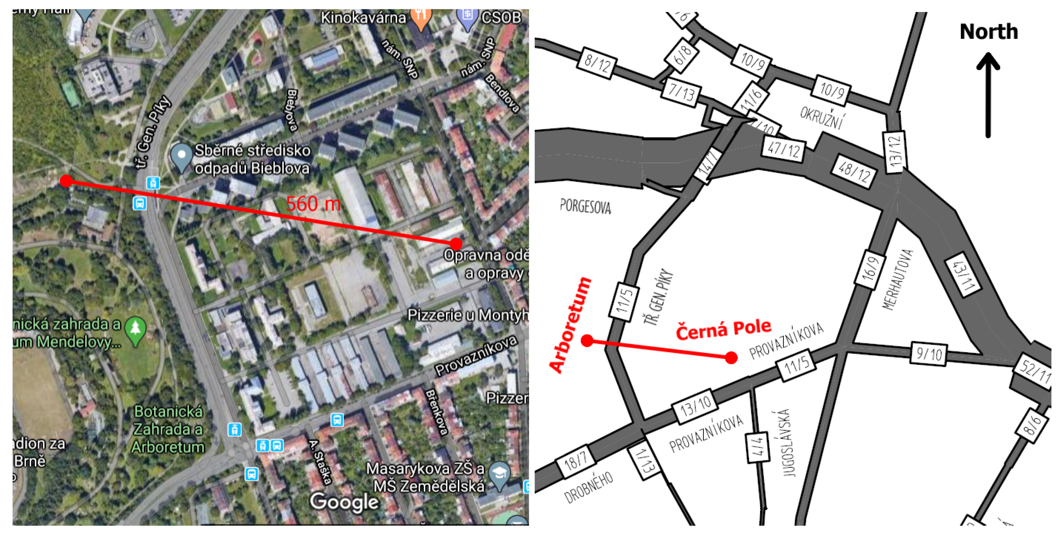
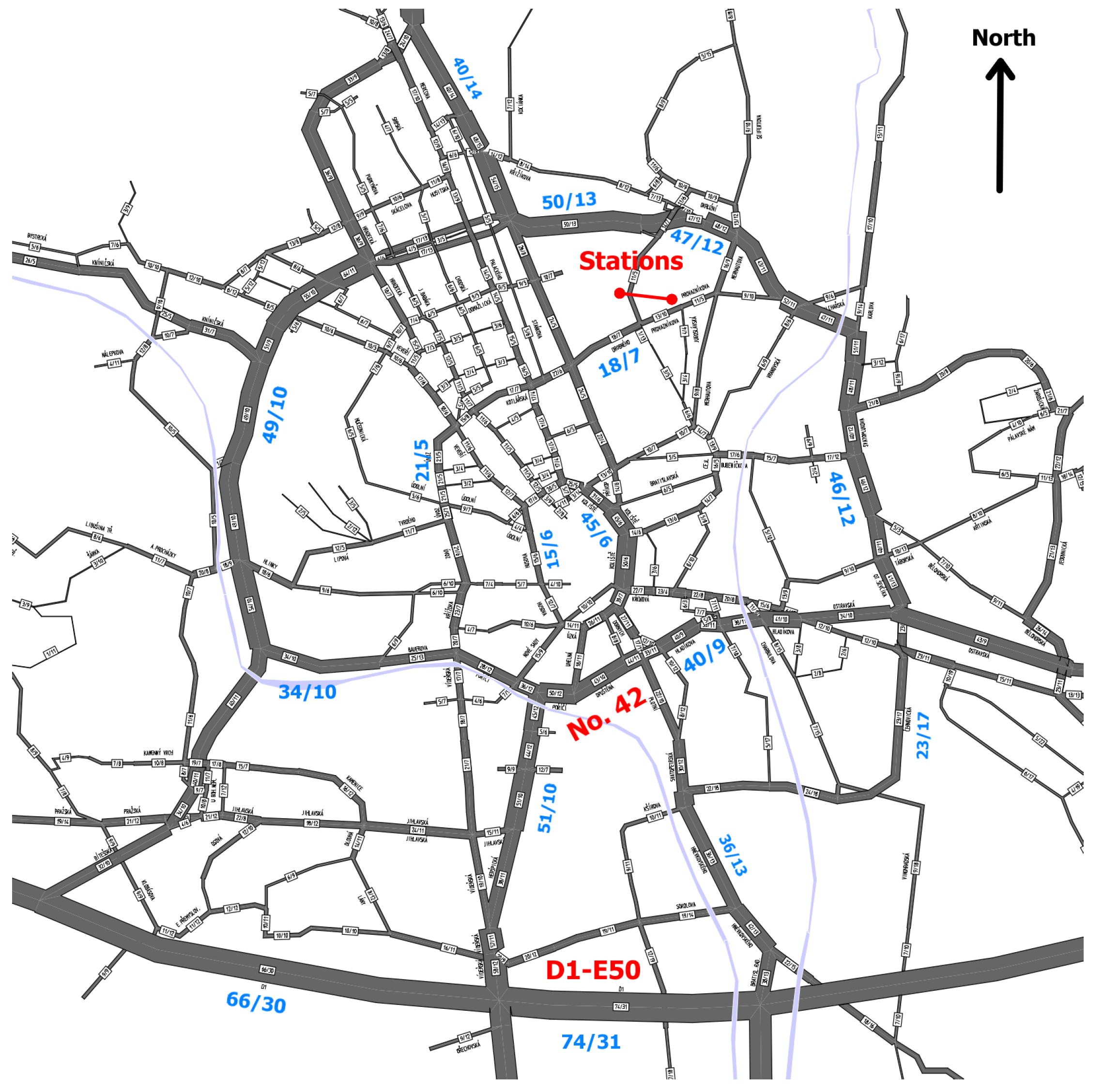
The monitoring station called “Arboretum” is located on top of a hill in the Mendel University botanical garden. East of the Arboretum station lie the premises of the University of Defence in Brno. On its campus, a mobile monitoring station was placed intentionally between the university buildings. Its working title, “Černá Pole”, was based on the name of the surrounding neighborhood. The distance between these two monitoring stations was 560 m; see the left part of Figure 1. Both stations are operated by the Department of Air Protection of the Environmental Protection Division of Brno City Municipality. This organization also provided the data. Between the botanical garden of Mendel University and the University of Defence campus, a busy road called Generála Píky street, which connects the Brno city center with the Brno-Lesná housing estate, runs in a northerly direction. Traffic volumes on individual roads surrounding the monitoring stations are depicted in Figure 1 on the right. The map with data represents the year of 2018 and was provided by Brněnské komunikace (BKOM). Every day, eleven-thousand vehicles use the Generála Píky street, 5 percent of which belong to freight transport. This volume will be denoted 11/5, and such a notation will be used in similar situations further on. Both monitoring stations are located approximately 0.5–1 km (about 1 km east, 0.5 km north, and 0.8 km north-west) from a major thoroughfare, the traffic volume of which is around 48/12; see Figure 1. At a distance of approximately 3.2 km south of the monitoring stations, Brno City Ring runs perpendicularly to this direction, denoted as Road No. 42 with a traffic volume of 40/9. In a more southern direction, at a distance of 6.5 km from the monitoring stations and parallel to the City Ring, the D1-E50 highway is located with a traffic volume of 74/31; see Figure 2.

2.2. Measured Variables

The measurements were taken every hour from 2 February to 20 April 2019. Both stations monitored levels of the PM${}_{10}$ fraction of suspended particulate matter, nitrogen oxides NO${}_x$, wind speed, maximum wind speed, wind direction, air temperature at 2 m above ground, air pressure, and humidity. For the purpose of statistical analysis of air pollution caused by PM${}_{10}$, the variables presented and explained in

Table 1. Notation for the measured variables.

Variable	Description
$\mathit{PM}{10}_t$	PM${}_{10}$ ($\mathsf{\mu }$g·m${}^{-3}$)
${\mathit{NOx}}_t$	NO${}_x$ ($\mathsf{\mu }$g·m${}^{-3}$)
$T_t$	temperature (${}^{\circ }$C)
$H_t$	humidity (%)
$V_t$	wind speed (m·s${}^{-1}$)
$D_t$	wind direction (degrees)
${\mathit{RH}}_t$	rush hours (a dummy variable equal to 1 for 7–10 AM, 3–5 PM;
	at other times, it is equal to 0)

were selected in compliance with previous statistical analyses based on daily mean values described in [23,24,25]. In this table, t denotes the hour the measurement was taken; $t=1,2,\cdots ,1872.$ (1872 measured hours correspond to 78 measured days). The time series of measurements contain 43 missing observations at the Arboretum station and 2 incomplete observations at the Černá Pole station.

Both stations were equipped with identical devices:

• For measuring concentrations of PM${}_{10}$: instrument manufactured by Environment SA, Model MP101M (MP101M is the automatic and real-time particulate monitor, compliant with ISO 10473:2000 and for PM${}_{10}$ US-EPA (EQPM-0404-151) and EN 12341 (I-CNR 087/2004, F-LCSQA). It allows the continuous and simultaneous measurement of fine dust, not influenced by the physico-chemical nature, color, or shape of particulates, in measurement ranges up to 10,000 $\mathsf{\mu }$g·m${}^{-3}$, with the lowest detectable limit of 0.5 $\mathsf{\mu }$g·m${}^{-3}$ (24 h average), with fiberglass tape (with 3 years of autonomy for continuous sampling with daily cycles) and with a measurement accuracy of ± 5%.).
• For measuring temperature and humidity: instrument made by Vaisala, Type HMP 155 with radiation shield DTR503 (HMP 155 (Vaisala) is the humidity and temperature probe compliant with the standards EN 61326-1 and EN 550022. Humidity measurement is based on the capacitive thin film HUMICAP${}^{\circledR }$ polymer sensor and temperature measurement on the resistive platinum sensors (Pt100). It allows the relative humidity (RH) measurement in the full range (0–100% RH) and with an accuracy in the range from −20 ${}^{\circ }$C to + 40 ${}^{\circ }$C ± (1.0 + 0.008 × reading)% RH. The accuracy temperature measurement is in the range from −80 ${}^{\circ }$C to +20 ${}^{\circ }$C ± (0.226 − 0.0028 × temperature) ${}^{\circ }$C and in the range from + 20 ${}^{\circ }$C to + 60 ${}^{\circ }$C ± (0.055 + 0.0057 × temperature) ${}^{\circ }$C).
• For measuring wind direction and speed: instrument manufactured by Gill Instruments Limited, type WindSonic (WindSonic is 2-axis ultrasonic wind sensor for true “fit and forget” wind sensing; it has no moving parts (alternative to conventional cup and vane or propeller wind sensors), compliant with the standard EN 61326:1998. It allows the wind speed measurement up to 60 m·s${}^{-1}$ with the accuracy ±2% (at 12 m·s${}^{-1}$) and wind direction measurement in the full circle with the accuracy $\pm 2^{\circ }$ (at 12 m·s${}^{-1}$).

Wind direction $D_t$ was measured as an oriented angle between the vector pointing north of the station and the observed wind direction vector pointing to the station corresponding to the maximum wind speed at hour $t.$ Rush hour ${\mathit{RH}}_t$ is a dummy variable equal to 1 for 7–10 AM, 3–5 PM; at other times, it is equal to 0.

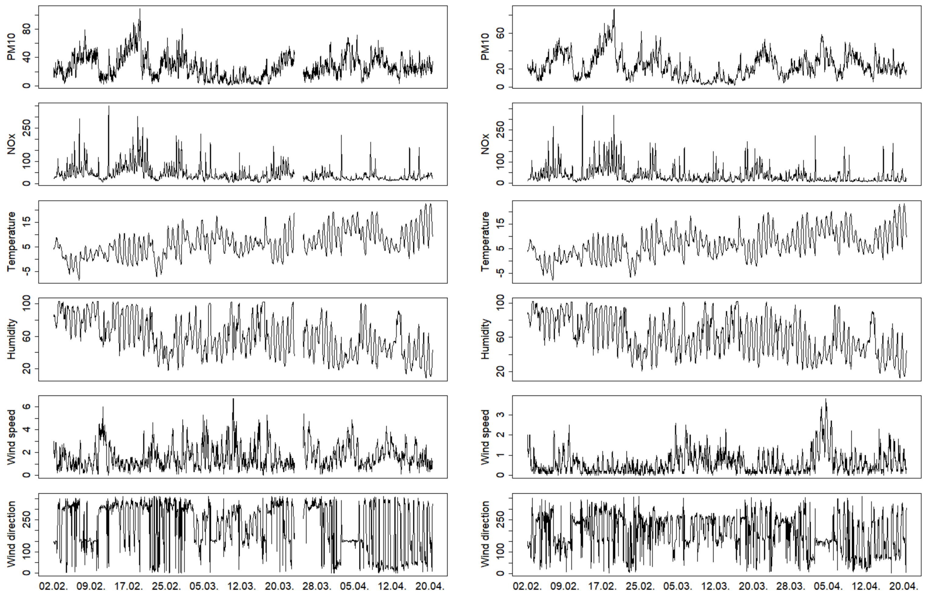
Figure 3 contains graphs with resulting measurements. Similar to [23,25], the previous two variables $V_t$ and $D_t$ were transformed into projections $V_{t}sin{D}_t$ and $V_{t}cos{D}_t$. As a result, it was possible to calculate the basic characteristics of wind direction and use them in further statistical analyses. The basic statistical characteristics of the analyzed data (number of observations n, mean, standard deviation, median, minimal and maximum observations, lower and upper quartiles, skewness, and kurtosis) for the selected variables, including their transformations, are presented in

Table 2. Descriptive statistics of variables (n—the number of observations; Mean—arithmetic mean; Median—median; St. dev.—standard deviation; Min—minimum value; Max—maximum value; $Q_{0.25}$—lower quartile; $Q_{0.75}$—upper quartile; Skewness—skewness, Kurtosis—kurtosis).

Arboretum	n	Mean	Median	St. dev.	Min	Max	${\mathbf{Q}}_{\mathbf{0}.\mathbf{25}}$	${\mathbf{Q}}_{\mathbf{0}.\mathbf{75}}$	Skewness	Kurtosis
$\mathit{PM}{\mathit{10}}_t$	1830	26.9	24.8	16.6	0.9	109.5	14.7	37.0	0.89	1.00
$\mathit{NO}{\mathit{x}}_t$	1827	43.5	32.2	36.2	4.7	348.7	22.1	50.2	2.89	11.74
$T_t$	1830	6.4	6.1	5.5	−8.6	22.5	2.5	9.8	0.30	−0.11
$H_t$	1829	59.6	58.0	23.2	9.0	103.0	41.0	77.0	0.14	−0.96
$V_t$	1830	1.6	1.4	1.1	0.0	6.7	0.9	2.2	1.15	1.19
$\sqrt{\mathit{PM}{\mathit{10}}_t}$	1830	4.9	5.0	1.6	0.9	10.5	3.8	6.1	0.04	−0.32
$V_{t}sin{D}_t$	1830	−0.38	−0.27	1.37	−6.69	3.05	−0.98	0.55	−0.80	0.97
$V_{t}cos{D}_t$	1830	0.46	0.68	1.26	−4.37	4.13	−0.40	1.27	−0.54	0.53
Černá Pole	n	Mean	Median	St. dev.	Min	Max	${\mathbf{Q}}_{\mathbf{0}.\mathbf{25}}$	${\mathbf{Q}}_{\mathbf{0}.\mathbf{75}}$	Skewness	Kurtosis
$\mathit{PM}{\mathit{10}}_t$	1871	23.5	21.2	13.5	2.1	87.3	13.5	31.5	0.86	0.85
$\mathit{NO}{\mathit{x}}_t$	1869	36.0	22.1	38.5	2.7	361.8	12.9	43.3	2.97	12.43
$T_t$	1872	6.8	6.4	5.6	−7.8	23.3	2.8	10.3	0.29	−0.18
$H_t$	1871	61.4	59.0	22.0	13.0	102.0	43.5	80.0	0.09	−1.03
$V_t$	1872	0.6	0.4	0.6	0.0	3.8	0.2	0.8	1.86	4.53
$\sqrt{\mathit{PM}{\mathit{10}}_t}$	1871	4.6	4.6	1.4	1.4	9.3	3.7	5.6	0.12	−0.36
$V_{t}sin{D}_t$	1872	0.05	−0.01	0.56	−1.98	2.22	−0.27	0.36	0.32	0.85
$V_{t}cos{D}_t$	1872	−0.25	−0.09	0.56	−3.44	1.02	−0.35	0.06	−2.11	5.83

for both the Arboretum and Černá Pole stations.

2.3. Methods

First, let us stress that the statistical data processing described below may resemble the standard procedure as described in Directive 2008/50/EC of the European Parliament and Council on ambient air quality and cleaner air for Europe, but it is a different one. To utilize the measured data more intensively and to get deeper statistical insights into the PM${}_{10}$ pollution level variations both in time and space, we used a finer time-granularity approach. Instead of using the “1 day averaging period” (i.e., one 24 h average per day), based on Annex XI of the European Directive, we used a moving 24 h average approach applied twenty-four times per day (i.e., every full hour). To bear resemblance to the common approach, the standard PM${}_{10}$ limit value of 50 $\mathsf{\mu }$g·m${}^{-3}$ was kept for our approach. Please note that with this “fine-granularity approach”, the number of exceedances calculated below cannot be directly compared to the standard national air pollution reports.

A test of equal proportions (see, e.g., [27]) to assess the (non-)equality of the relative frequencies of the moving 24 h average values exceeding the limit level was applied to data collected by the Arboretum and Černá Pole stations.

Parallel measurements of PM${}_{10}$ and NO${}_x$ from both stations were compared using the Passing–Bablok test [28]. It is a robust, nonparametric method for fitting a straight line to two variables X (PM${}_{10}$, Arboretum station) and Y (PM${}_{10}$, Černá Pole station). This is accomplished by estimating a linear regression line and testing whether the intercept is zero and the slope is one. If the hypothesis that the intercept is zero and the slope is one is not rejected, the measurements can be considered comparable. Otherwise, the measurements are not comparable.

A regression model (see, e.g., [29,30]) for the prediction of pollution by PM${}_{10}$ was created, and regressors were selected using the backward selection method. In statistics, backward selection is a method of fitting regression models in which the choice of regressors is carried out by an automatic procedure. It involves starting with all candidate variables (regressors), testing the deletion of each variable using a chosen model fit criterion, deleting the variable (if any) whose loss gives the most statistically insignificant deterioration of the model fit, and repeating this process until no further variables can be deleted without a statistically significant loss of fit. The common choice of the model fit criterion is the Akaike information criterion (AIC); see, e.g., [29].

With respect to outputs of the regression model, wind direction and speed were analyzed, and mean values of PM${}_{10}$ for various wind directions were compared using the analysis of variance [29].

Hourly measurements of the following variables were crucial for the construction of the regression model: $\mathit{PM}{10}_t$, wind speed $V_t$, wind direction $D_t$, temperature $T_t$, and humidity $H_t$. It is clearly visible from Figure 3 that wind speed and wind direction are very different between the stations (their behavior is affected mainly by the built-up area geometry), and the values of these two variables have a great impact on the local PM${}_{10}$ pollution levels.

The details of the statistical methods can be found in [29,30]. All the calculations were carried out in the R environment [31] using the openair [32], forecast [33], mcr [34], MASS [35], and car [36] packages.

3. Results

3.1. Frequency of Limit Value Exceedances for a Moving Average

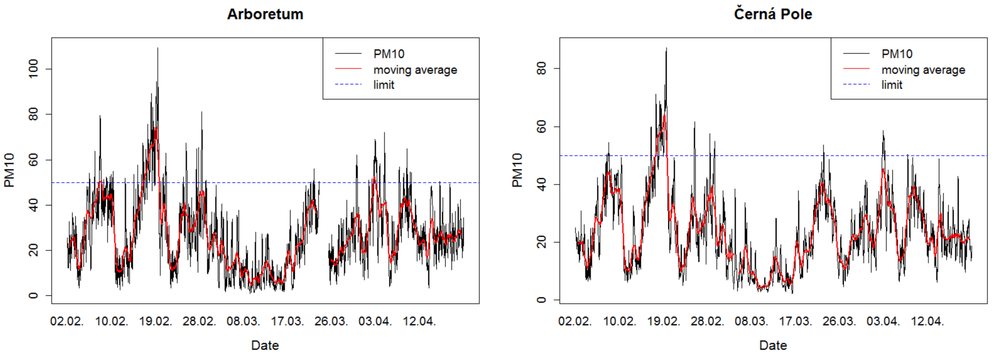
Figure 4 represents hourly averages and 24 h moving averages of PM${}_{10}$ concentrations measured at the Arboretum and Černá Pole stations, together with the limit value.

Considering the missing data, $n=1757$ measurements were performed at each of the two stations during the monitoring period (only parallel measurements without missing values are considered). At the Arboretum station, the limit value of 50 $\mathsf{\mu }$g·m${}^{-3}$ was exceeded by 100 moving average values calculated for every hour of each day, and the relative frequency was equal to 0.0569. At the Černá Pole station, the limit value was exceeded by 53 calculated values, and the relative frequency was equal to 0.0302. The 95% confidence interval for the probability of exceeding the limit value of 50 $\mathsf{\mu }$g·m${}^{-3}$ is (0.0514, 0.0624) in the case of the Arboretum station and (0.0260, 0.0342) in the case of the Černá Pole station.

The statistical comparison of relative frequencies of exceeding the limit value at the Arboretum station (0.0569) and at the Černá Pole station (0.0302) shows that the values can be considered different at the significance level of 5%; the corresponding p-value is $0.0001$.

As a side note, it may be of interest to experts dealing with a number of exceedances determined by the “one day averaging period” (i.e., just one 24 h average per day) based on Annex XI of Directive 2008/50/EC that this approach (as applied by the Czech Hydro-meteorological Institute) resulted in only five days with the PM${}_{10}$ limit of 50 $\mathsf{\mu }$g·m${}^{-3}$ exceeded for the processed period. The finer-granularity approach used in this paper results in eight days with one or more 24 h moving averages (of 24 hourly ones calculated daily) exceeding the same limit.

The observational period used in this study is not long enough to draw robust conclusions, but the above stated difference of five and eight exceedances, if projected to the full calendar year, could mean that for a case of a calendar year with 35 exceedances officially reported using the European Directive approach, there could be some 56 days detected with the same limit exceeded if 24 h moving averages calculated hourly are considered in our approach. In another view, the above stated difference in the number of days with detected exceedances could mean that 35 days with the exceeded limit of any of the hourly calculated 24 h moving averages in a day might be reached in a calendar year just when as low as 22 days with the limit exceedance reported based on the current national practice are reported. Without elaborating on the details, it should be noted that a compromise between the two mentioned approaches is needed to fine tune the reporting of exceedances.

It is obvious that our finer-granularity approach exposes a weakness of the official reporting practice. For example, currently, a calendar day with 23 detected exceedances of the 24 h moving average would be neglected in the official reporting if the 24 h average calculated at midnight was not exceeding the limit value. Similarly, a day would not be included in the official reporting in the case that the limit value would be exceeded only once during the day, and this was not the midnight value of the 24 h average. In such a situation, 23 of 24 possible cases would be neglected. Therefore, the current normative situation can be seen as under-representing real pollution levels and therefore to be a breach of the widely accepted precautionary principle used for environment impact assessments.

In conclusion, it can be highlighted that the discrepancy between the two exceedance assessments increases with lowering the PM${}_{10}$ pollution levels. The reason is that the probability of omitting such “exceedance” days in the annual statistics increases with lowering the number of 24 h moving averages exceeding the limit from 23 to one during a single calendar day.

3.2. Comparison of PM${}_{10}$ Measurements

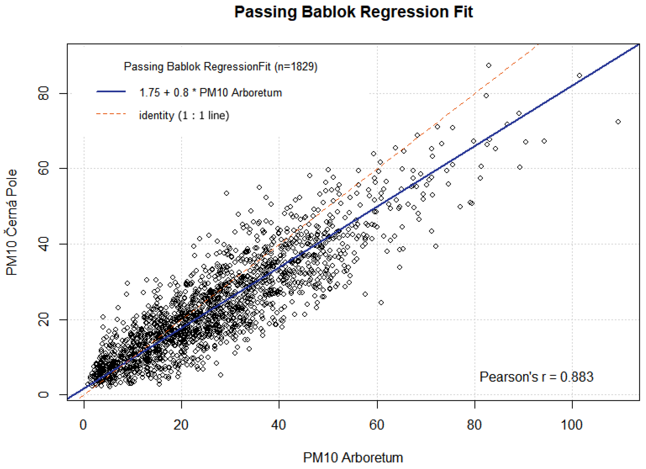
A comparison of parallel PM${}_{10}$ measurements between the Arboretum and Černá Pole stations can be roughly assessed from the top row graphs in Figure 3. A detailed comparison was carried out using the non-parametric Passing–Bablok test. The robust regression line for PM${}_{10}$ values at Arboretum and Černá Pole stations is defined by the following equation:

$$\mathit{PM}{10}_t^{Č\mathrm{ern}á\mathrm{Pole}}=1.754+0.802·\mathit{PM}{10}_t^{\mathrm{Arboretum}}.$$

(1)

Results of the Passing–Bablok test together with the regression line are presented in Figure 5. The 95% confidence intervals for parameters of the regression line are (1.299, 2.215) in the case of the intercept and (0.783, 0.822) in the case of the slope. The null hypothesis that the parallel measurements are not statistically significantly different (the intercept equals zero, and the slope equals one) was rejected at the significance level of 5%. The test revealed a statistically significant difference between both parallel measurements.

Furthermore, the correlation coefficients were determined. Pearson’s correlation coefficient between $\mathit{PM}{10}_t^{Č\mathrm{ern}á\mathrm{Pole}}$ and $\mathit{PM}{10}_t^{\mathrm{Arboretum}}$ is 0.883 (p-value ≅ 0), and Spearman’s correlation coefficient is 0.872 (p-value ≅ 0). Both correlation coefficients are significantly different from zero. The results show that with a 10 $\mathsf{\mu }$g·m${}^{-3}$ increase of PM${}_{10}$ pollution level at the Arboretum station, there is on average only an 8.02 $\mathsf{\mu }$g·m${}^{-3}$ increase at the Černá Pole station. The results obtained by the robust Passing–Bablok test show how the two nearby monitoring stations differ in the level of PM${}_{10}$ pollution.

3.3. Comparison of NO${}_x$ Measurements

Transport is one of the main sources of nitrogen oxides. The authors in [37] discussed the presence of NOx from vehicle exhaust in the composition of PM. Using correlation analysis, we assessed the statistical relationship between PM${}_{10}$ and nitrogen oxides NO${}_x$. Spearman’s correlation coefficient between PM${}_{10}$ values and NO${}_x$ has a value of 0.478 (p-value ≅ 0) for the Arboretum station and 0.372 (p-value ≅ 0) for Černá Pole station. From the above values, it is clear that in the case of the Arboretum station, the correlation coefficient is higher (p-value 0.00017). We will now compare the NO${}_x$ values for both stations using the Passing–Bablok test, similar to the PM${}_{10}$ comparison. We get an estimate of the regression function in the form:

$${\mathit{NOx}}_t^{Č\mathrm{ern}á\mathrm{Pole}}=-8.212+1.014·{\mathit{NOx}}_t^{\mathrm{Arboretum}}.$$

(2)

The 95% confidence intervals for the parameters of the regression line are (−8.898, −7.531) in the case of the intercept and (0.994, 1.034) in the case of the slope. The results of the robust Passing–Bablok test show that the two nearby monitoring stations differ in the level of NO${}_x$. The difference is due to the non-zero value of the intercept in the estimated regression function Equation (2). The hypothesis that the slope in the regression function has a value of one is not rejected.

Pearson’s correlation coefficient between ${\mathit{NOx}}_t^{Č\mathrm{ern}á\mathrm{Pole}}$ and ${\mathit{NOx}}_t^{\mathrm{Arboretum}}$ is 0.933 (p-value ≅ 0), and Spearman’s correlation coefficient is 0.901 (p-value ≅ 0). Both correlation coefficients are significantly different from zero.

3.4. Regression Models for PM${}_{10}$ Prediction

The regression model for PM${}_{10}$ prediction was constructed with respect to the previously published results in [23,24,25]. The following auxiliary variables were used for the prediction of $\mathit{PM}{10}_t$: temperature $T_t$, humidity $H_t$, wind speed $V_t$, wind direction $D_t$, rush hours ${\mathit{RH}}_t$, and their transformations: time differences of temperatures $T_t-T_{t-1}$ and $T_{t-1}-T_{t-2}$, time differences of humidity $H_t-H_{t-1}$, and transformations of wind direction and wind speed $V_{t}sin{D}_t$, $V_{t}cos{D}_t$, which made it possible to incorporate wind directions into the regression model.

Since the relation between PM${}_{10}$ value and atmospheric pressure proved to be statistically insignificant in previous and current analyses, the atmospheric pressure variable was not used in the regression model. Pearson’s correlation coefficient is 0.082, and Spearman’s correlation coefficient is 0.109. Despite the fact that both correlation coefficients are, due to the large number of observations, statistically significant at the significance level of 5%, based on Pearson’s correlation coefficient, it can be concluded that atmospheric pressure explains only 0.68% of the variability of the $\mathit{PM}{10}_t$ variable. On that account, atmospheric pressure is not included in further analyses.

With regard to the article [25], three regression models were studied. There were two generalized autoregressive linear models (GALM) [30]; one with the gamma distribution and canonical link function (which is the reciprocal function for gamma distribution), the other with the gamma distribution and log-link function. The third model was the linear regression model for the $\sqrt{\mathit{PM}{10}_t}$ variable (see [7,25]), and it worked best for the hourly data. All three models were computationally processed, then their comparison was performed using the coefficients of determination; their graphical comparison was performed, and the third model proved to be the most suitable. Due to the scope of the article, the results of the first two models are not presented. One of the reasons why the third model was used was that graphs rendered using Q-Q plots and the Anderson–Darling goodness-of-fit test showed that the distribution of $\sqrt{\mathit{PM}{10}_t}$ is very close to a normal distribution at both stations. The regressors were selected using the backward selection method and the AIC criterion (Akaike information criterion). The final model contained eight parameters ${\beta }_1,{\beta }_2,\cdots ,{\beta }_8$ and random error ${ϵ}_t$ for observations in time $t=1,2,\cdots ,n$, where n is the number of hourly observations. It is of the form:

$$\begin{array}{cc}\hfill \sqrt{\mathit{PM}{10}_t}=& {\beta }_1+{\beta }_2\sqrt{\mathit{PM}{10}_{t-1}}+{\beta }_3(T_t-T_{t-1})+{\beta }_4(T_{t-1}-T_{t-2})+\hfill \\ \hfill & +{\beta }_5(H_t-H_{t-1})+{\beta }_6{V}_{t-1}sin{D}_{t-1}+{\beta }_7{V}_{t-1}cos{D}_{t-1}+{\beta }_8{\mathit{RH}}_{\mathit{t}}+{ϵ}_t.\hfill \end{array}$$

(3)

The adjusted coefficient of determination $R_{adj}^2$ was used for assessing the suitability of the statistical relation between the $\sqrt{\mathit{PM}{10}_t}$ response variable and the auxiliary variables incorporated into the model. Its values were high and statistically significant (0.806 for the Arboretum station and 0.918 for the Černá Pole station). Standardized residuals did not show any extreme deviations in comparison to the previous two GALM models.

Estimated coefficients (with their standard errors in parentheses) can be found in

Table 3. Estimates of the linear models; standard errors are in parentheses.

		Dependent Variable:
		$\sqrt{\mathit{PM}{\mathbf{10}}_{\mathbf{t}}}$
Parameter	Variable	Arboretum	Černá Pole
${\beta }_1$		0.593 ***	0.241 ***
		(0.060)	(0.035)
${\beta }_2$	$\sqrt{\mathit{PM}{10}_{t-1}}$	0.878 ***	0.946 ***
		(0.011)	(0.007)
${\beta }_3$	$T_t-T_{t-1}$	0.118 ***	0.117 ***
		(0.033)	(0.017)
${\beta }_4$	$T_{t-1}-T_{t-2}$	−0.094 ***	−0.052 ***
		(0.024)	(0.012)
${\beta }_5$	$H_t-H_{t-1}$	0.006	0.011 ***
		(0.005)	(0.003)
${\beta }_6$	$V_{t-1}sin{D}_{t-1}$	0.071 ***	0.085 ***
		(0.014)	(0.018)
${\beta }_7$	$V_{t-1}cos{D}_{t-1}$	0.002	0.049 ***
		(0.015)	(0.018)
${\beta }_8$	${\mathit{RH}}_{\mathit{t}}$	0.117 ***	0.054 **
		(0.040)	(0.022)
Number of observations n		1824	1866
R${}^2$		0.807	0.919
Adjusted R${}^2$		0.806	0.918
Residual Std. Error		0.722 (df = 1816)	0.402 (df = 1858)
F Statistic		1,083.102 *** (df = 7; 1816)	2,993.700 *** (df = 7; 1858)

Note: * p < 0.1; ** p < 0.05; *** p < 0.01.

; in the column Arboretum for the Arboretum station and in the column Černá Pole for the Černá Pole station. Moreover, there are the number of observations n (there were missing observations in the data), the coefficient of determination $R^2$, the adjusted coefficient of determination $R_{adj}^2$, the residual standard error, the F statistic, and the corresponding degree of freedom $\mathit{df}=(\mathit{df}1;\mathit{df}2)$. The statistical significance of the coefficients is denoted by *, where the number of asterisks indicates the respective p-values corresponding to the statistical significance of the respective coefficient. It can be seen that the proposed model Equation (3) is suitable for the description of the studied statistical relationship between $\sqrt{\mathit{PM}{10}_t}$ and the selected regressors for each of the stations. The coefficient of determination $R^2$ and the adjusted coefficient of determination $R_{adj}^2$ are high for both stations, and the value of the F statistic describing the suitability of the model is also statistically significant at the significance level of 1%. Moreover, Table 3 shows that all coefficients of both statistical models are significantly different from zero at least at the significance level of 5% with the exception of coefficients ${\beta }_5$ and ${\beta }_7$ for the Arboretum station.

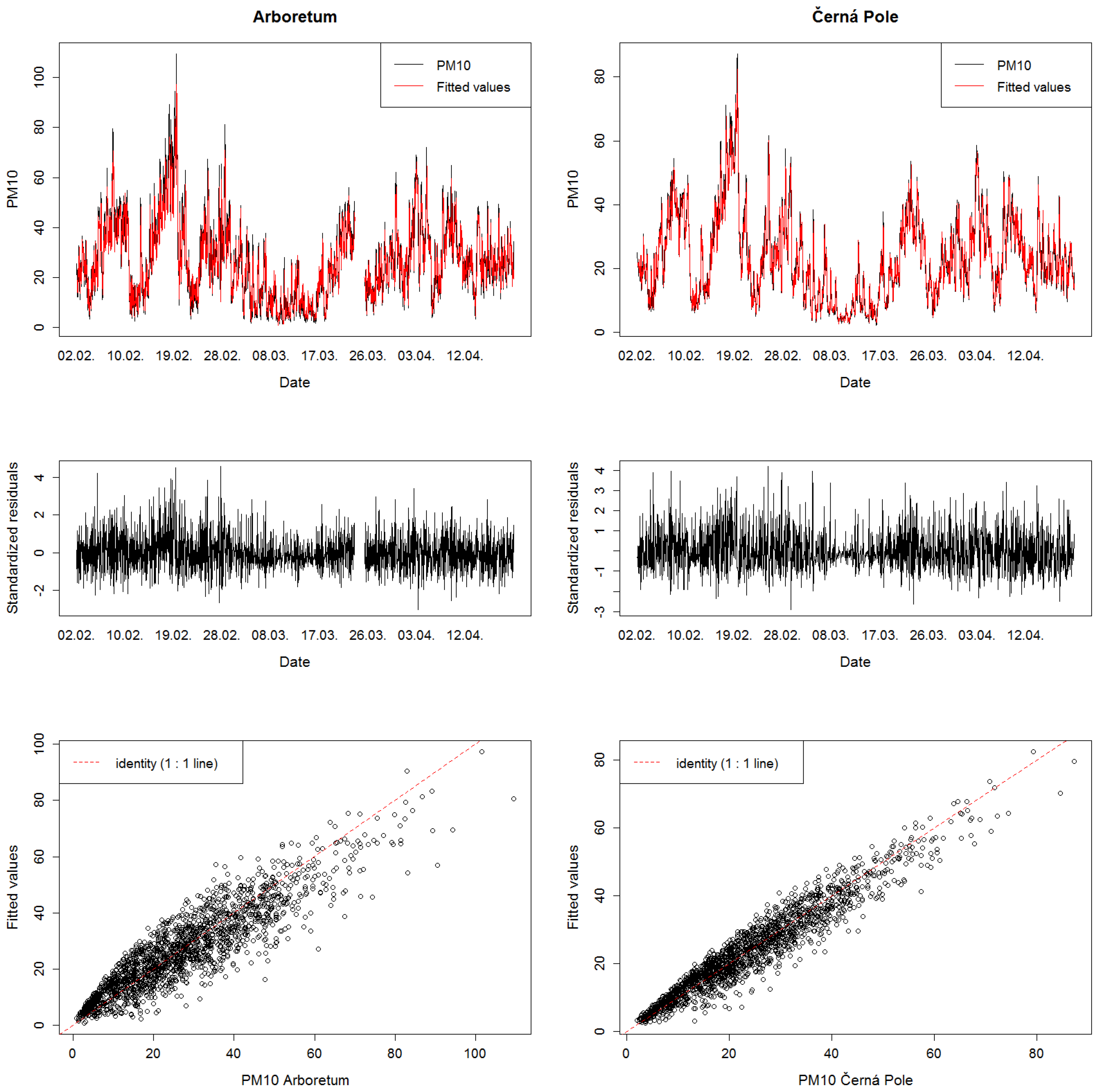
Agreement between the prediction model Equation (3) and the data can be visually assessed from Figure 6, where the observed and predicted (fitted) $\mathit{PM}{10}_t$ values are in the top row, the corresponding standardized residuals are in the middle row, and graphs of measured and fitted values of $\mathit{PM}{10}_t$ are in the bottom row. It is evident from the graphs (especially from the graphs showing the measured values versus the fitted ones) that the estimated models describe the development of PM10 with sufficient accuracy. The model for the Černá Pole station has greater accuracy than the model for the Arboretum station. This conclusion corresponds to the values of $R^2$ in Table 3, where $R^2=0.919$ for the Černá Pole station and $R^2=0.807$ for the Arboretum station.

Agreement between the estimated parameters of model Equation (3) for Arboretum and Černá Pole stations can be assessed using the regression analysis methods and the F statistic. This statistic can also be modified in order to test the equality of the corresponding regression parameters; see [29]. The value of the F statistics for comparing the two models is $F=5.5039$, and the corresponding p-value is $6.193\times {10}^{-7}$; i.e., both models are significantly different from each other. A detailed comparison of the parameters of both models from Table 3 can be found in

Table 4. Tests of equal parameters and model comparison.

Parameter	Variable	F-Test	p-Value
${\beta }_1$		25.19828	5.41837$\times {10}^{-7}$
${\beta }_2$	$\sqrt{{\mathit{PM}}_{t-1}}$	25.51096	4.61270$\times {10}^{-7}$
${\beta }_3$	$T_t-T_{t-1}$	0.00008	0.99266
${\beta }_4$	$T_{t-1}-T_{t-2}$	2.65500	0.10331
${\beta }_5$	$H_t-H_{t-1}$	0.80706	0.36905
${\beta }_6$	$V_{t-1}sin{D}_{t-1}$	0.26454	0.60705
${\beta }_7$	$V_{t-1}cos{D}_{t-1}$	2.56720	0.10919
${\beta }_8$	${\mathit{RH}}_{\mathit{t}}$	1.96325	0.16125
All parameters		5.5039	6.193$\times {10}^{-7}$

. It is clear that both models differ only in parameters ${\beta }_1$ (intercept, p-value ≅ 0) and ${\beta }_2$ (p-value ≅ 0), which corresponds to the value of the lagged transformed variable $\sqrt{\mathit{PM}{10}_{t-1}}$; i.e., the PM${}_{10}$ pollution level from the previous hour.

3.5. Influence of Wind on PM${}_{10}$ Levels

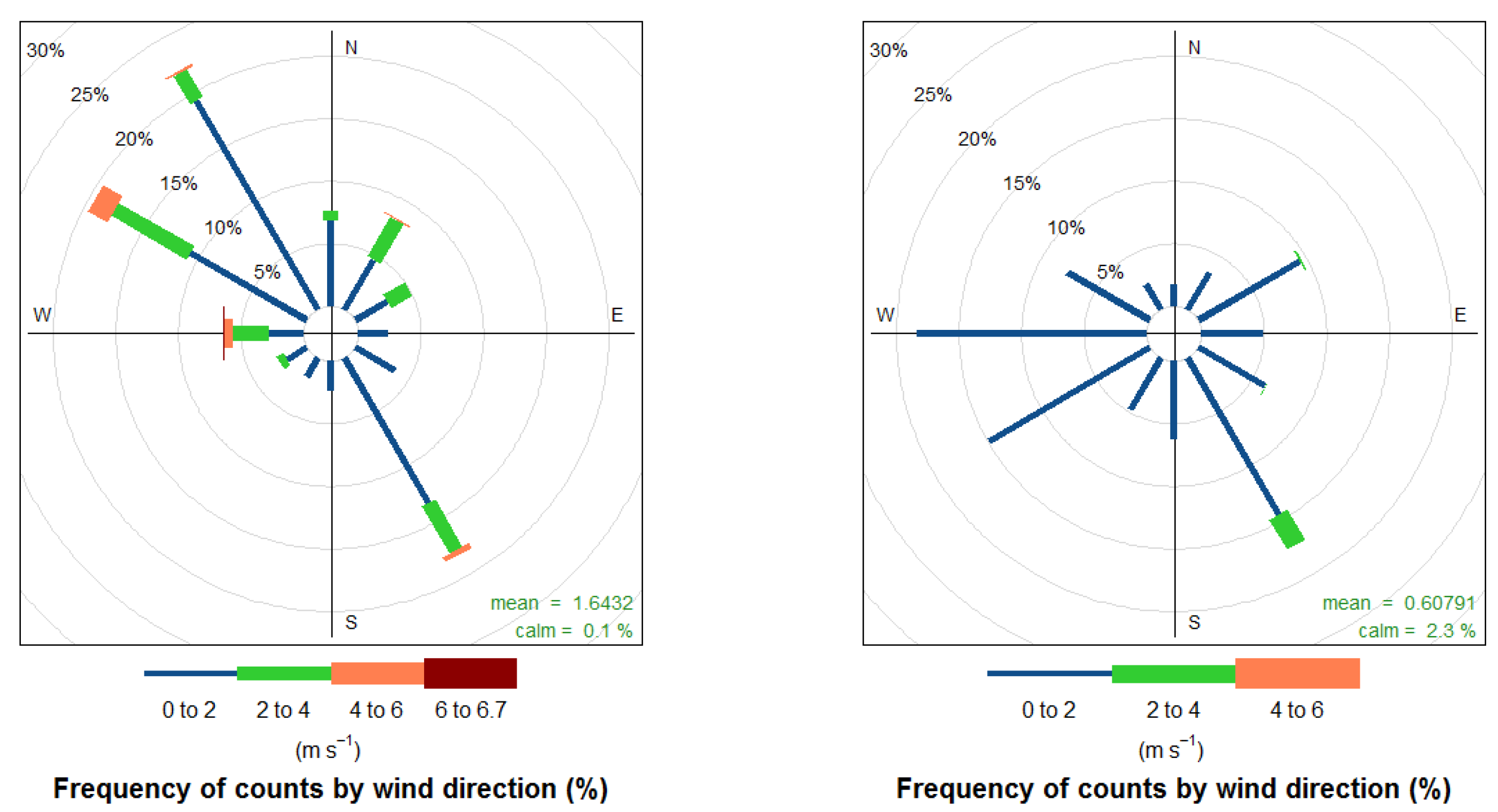
For the purpose of the statistical analysis of the influence of wind speed $V_t$ and wind direction $D_t$ on PM${}_{10}$ air pollution at both stations, possible wind directions ranging from zero to 360 degrees (clockwise) were divided into 12 sections $\langle 345,15),\langle 15,45),\langle 45,75),\cdots ,\langle 315,345)$ by 30 degrees. Furthermore, a wind rose representing the frequency of counts by wind direction and wind speed was created. Subsequently, the basic statistical characteristics of PM${}_{10}$ levels were calculated for each section. One-way analysis of variance was carried out in order to compare mean values of air pollution in individual directions. Wind roses for both the Arboretum and Černá Pole stations are presented in Figure 7. It is clear from the wind rose graphs that the characteristics describing the wind speed and direction are different for both stations. At the Arboretum station located in the open space of the botanical garden, higher wind speeds can be observed, and the northwest and southeast directions predominate. At the Černá Pole station, which is located in a built-up area, the measured wind speeds are lower, and the northeast wind direction is almost absent. Like the Arboretum station, there is a southeast wind direction. These differences are caused by the surrounding built-up area (especially buildings) of the Černá Pole station.

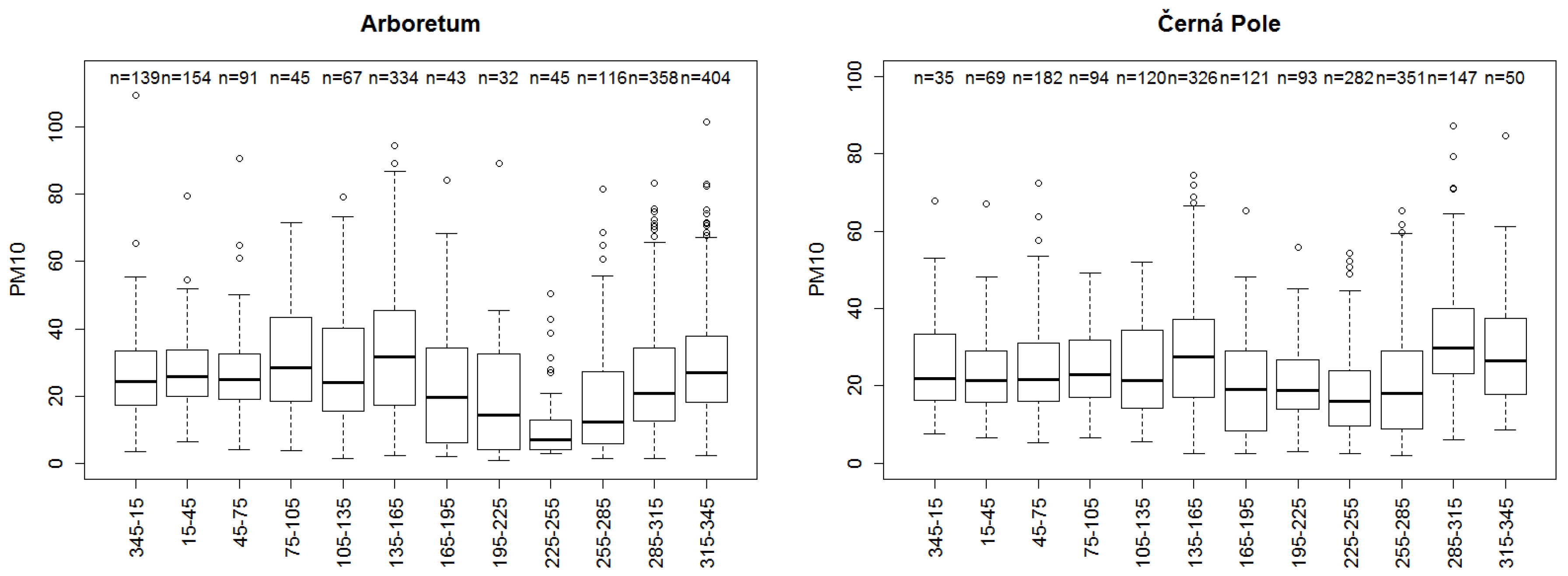
Boxplots comparing pollution levels in individual sections can be found in Figure 8 for both stations. Furthermore,

Table 5. Descriptive statistics for PM${}_{10}$ by wind direction: Arboretum station (n—the number of observations; Mean—arithmetic mean; Median—median; St. dev.—standard deviation; Min—minimum; Max—maximum; $Q_{0.25}$—lower quartile; $Q_{0.75}$—upper quartile).

Degrees	n	Mean	Median	St. dev.	Min	Max	${\mathit{Q}}_{0.25}$	${\mathit{Q}}_{0.75}$
all	1828	27.0	24.8	16.6	0.9	109.5	14.7	37.0
345–15	139	27.0	24.4	14.4	3.4	109.5	17.4	33.4
15–45	154	27.0	25.9	11.3	6.5	79.5	19.8	33.5
45–75	91	26.6	25.0	13.3	4.0	90.5	19.1	32.5
75–105	45	31.5	28.5	16.7	3.8	71.5	18.4	43.3
105–135	67	28.0	23.9	17.3	1.4	79.2	15.5	40.1
135–165	334	32.2	31.6	18.2	2.2	94.4	17.4	45.3
165–195	43	22.8	19.7	19.3	1.9	84.3	6.2	34.4
195–225	32	19.7	14.3	19.6	0.9	89.3	4.2	31.9
225–255	45	11.9	7.0	11.4	2.8	50.4	4.2	12.9
255–285	116	18.5	12.4	17.2	1.4	81.4	5.8	27.0
285–315	358	24.7	20.8	16.6	1.4	83.2	12.6	34.4
315–345	404	29.1	27.0	15.5	2.2	101.6	18.3	37.8

contains descriptive statistics for individual sections for the Arboretum station, whereas

Table 6. Descriptive statistics for PM${}_{10}$ by wind direction: Černá Pole station (n—the number of observations; Mean—arithmetic mean; Median—median; St. dev.—standard deviation; Min—minimum; Max—maximum; $Q_{0.25}$—lower quartile; $Q_{0.75}$—upper quartile).

Degrees	n	Mean	Median	St. dev.	Min	Max	${\mathit{Q}}_{0.25}$	${\mathit{Q}}_{0.75}$
all	1870	23.5	21.1	13.5	2.1	87.3	13.5	31.5
345–15	35	25.6	21.9	13.7	7.7	67.8	16.3	33.4
15–45	69	22.8	21.5	10.7	6.6	67.0	15.9	29.0
45–75	182	24.3	21.6	11.7	5.3	72.3	16.1	30.9
75–105	94	25.2	23.0	10.1	6.7	49.2	17.1	31.8
105–135	120	24.6	21.4	12.8	5.6	52.0	14.4	34.1
135–165	326	28.2	27.5	14.8	2.5	74.5	17.2	37.1
165–195	121	19.6	19.1	12.9	2.4	65.3	8.3	29.1
195–225	93	20.2	18.8	9.5	3.0	55.8	14.0	26.8
225–255	282	17.4	16.1	9.8	2.6	54.2	9.6	23.9
255–285	351	20.4	18.2	13.5	2.1	65.2	8.8	29.1
285–315	147	32.6	29.9	15.1	6.0	87.3	23.3	40.1
315–345	50	29.8	26.4	14.9	8.7	84.6	18.0	38.0

contains the same information from the Černá Pole station. Using one-way analysis of variance, the null hypothesis claiming that the mean level of PM10 air pollution is the same in all 12 sections was tested against an alternative hypothesis stating that levels of pollution show statistically significant differences due to the effect of various wind directions. The analysis of variance was applied to the $\sqrt{\mathit{PM}{10}_t}$ variable, which has a normal distribution for data from individual sections. As for the Arboretum station, the value of the test statistics $F=17.07$ and p-value is zero, with degrees of freedom 11 and 1816. For the Černá Pole station, this statistic equals $F=22.26$; the p-value is zero, with degrees of freedom 11 and 1858. On that account, it may be argued that each station showed statistically significant differences in the mean values of air pollution in terms of wind direction. Since each station provided evidence on statistically significant differences in the mean values of air pollution caused by PM${}_{10}$, Tukey’s honest significance test was performed for each station in order to identify pairs of monitored sections that exhibit substantially different air pollution levels. The test compared 66 section pairs; for the purpose of its interpretation in this paper, only comparisons of sections with the highest and lowest pollution levels were selected.

Regarding the Arboretum station, mean values of pollution levels resulting from measured values and wind directions are presented in Table 5; the corresponding graph can be found in Figure 8 on the left. As can be derived from the table, air pollution with the highest mean value of 32.2 $\mathsf{\mu }$g·m${}^{-3}$ and the highest median value of 31.6 $\mathsf{\mu }$g·m${}^{-3}$ was measured in the direction of 135 to 165 degrees. Another two sections with the mean value of pollution higher than 28 $\mathsf{\mu }$g·m${}^{-3}$ and the median value higher than 26 $\mathsf{\mu }$g·m${}^{-3}$ were those of 75–105 degrees and 315–345 degrees. Tukey’s honest significance test did not prove statistically significant differences in the mean values of air pollution between pairs consisting of the above-mentioned three sections with the highest pollution levels. On the contrary, the section with the lowest pollution levels was the one of 225–255 degrees, where the mean value of the pollution level was 11.9 $\mathsf{\mu }$g·m${}^{-3}$, and the median was 7 $\mathsf{\mu }$g·m${}^{-3}$. Low levels of pollution with the mean value lower than 23 $\mathsf{\mu }$g·m${}^{-3}$ and the median lower than 20 $\mathsf{\mu }$g·m${}^{-3}$ were found in four sections between 165 and 285 degrees. Tukey’s honest significance test proved statistically significant differences in the mean value of pollution levels between the section of 135–165 degrees and each of the four sections ranging from 165 to 285 degrees.

Similarly, the mean values of pollution levels measured at the Černá Pole station with regard to the wind direction are presented in Table 6; the corresponding graph is in Figure 8 on the right. This table shows that the air pollution with the highest mean value of 32.6 $\mathsf{\mu }$g·m${}^{-3}$ and the highest median value of 29.9 $\mathsf{\mu }$g·m${}^{-3}$ was measured in the direction of 285 to 315 degrees. Another two sections with the mean value of pollution higher than 28 $\mathsf{\mu }$g·m${}^{-3}$ and the median value higher than 26 $\mathsf{\mu }$g·m${}^{-3}$ were those of 315–345 degrees and 135–165 degrees. As in the case of the Arboretum station, Tukey’s honest significance test performed for the Černá Pole station did not return statistically significant differences in the mean values of air pollution between pairs consisting of the above-mentioned three sections with the highest pollution levels. On the contrary, the section with the lowest pollution levels was the one of 225–255 degrees, where the mean value of the pollution level was 17.4 $\mathsf{\mu }$g·m${}^{-3}$ and the median was 16.1 $\mathsf{\mu }$g·m${}^{-3}$. It follows from the above that the section with the lowest pollution levels is the same for both stations. Low pollution levels with the mean value lower than 23 $\mathsf{\mu }$g·m${}^{-3}$ and the median lower than 20 $\mathsf{\mu }$g·m${}^{-3}$ were measured again in four sections within the range of 165–285 degrees. Tukey’s honest significance test proved statistically significant differences for each pair of these sections; the first section was always selected from the three sections with the highest mean value of air pollution, and the second one was selected among the four sections with the lowest mean value within the range of 165–285 degrees.

4. Discussion

The analysis of the results of parallel measurements obtained at two stations that are 560 m from each other and located in the northern parts of Brno City showed that the monitored levels of PM${}_{10}$ vary considerably between the locations; at the Arboretum station, which lies in an open area in a park, as well as at the Černá Pole station, which is placed on a campus and surrounded by low-rise buildings. A comparison of the relative frequencies of exceeding the level of 50 $\mathsf{\mu }$g·m${}^{-3}$ was performed. From the statistical point of view, these frequencies differed significantly between the stations; at the Černá Pole station, the frequencies of exceeding set limits were significantly lower than at the Arboretum station. Thus, the significant differences between the levels of measurement of PM values at both stations are influenced mainly by the built-up area geometry.

A comparison of parallel measurements using the Passing–Bablok test also showed that the values of air pollution caused by PM${}_{10}$ measured at the Černá Pole station surrounded by low-rise buildings were lower than those monitored in the open-area of the Arboretum station. Whereas at the Arboretum station, PM${}_{10}$ pollution levels increased by 10 $\mathsf{\mu }$g·m${}^{-3}$, at the Černá Pole station, they grew on average only by 8.02 $\mathsf{\mu }$g·m${}^{-3}$.

Based on the results of the correlation analysis between the values of PM${}_{10}$ and NO${}_x$, it can be stated that there is a statistical link between the monitored variables. Spearman’s correlation coefficient for the Arboretum station was significantly higher than for the Černá Pole station. The Passing–Bablok test applied to NO${}_x$ values then showed that the pollution levels for the monitored stations were not the same. The NO${}_x$ values from the Černá Pole station were lower than at the Arboretum station, by approximately 8.2 $\mathsf{\mu }$g·m${}^{-3}$. The results show the effect of built-up geometry on the level of pollution. PM${}_{10}$ and NO${}_x$ values were higher for the Arboretum station located in a park near a busy street than for Černá Pole located in a built-up area. The obtained results correspond to the conclusions published, e.g., in [22].

During the analyses of hourly data on air pollution caused by PM${}_{10}$, the presented statistical models proved that PM${}_{10}$ air pollution is influenced, above all, by temperature change; i.e., first, by its drop with a two hour delay, then by its rise in the next hour. At the Arboretum station, humidity change did not prove to be a statistically significant parameter; however, at the Černá Pole station, quite the contrary was the case. A positive value of the regression parameter 0.011, which was statistically significantly different from zero for the Černá Pole station, indicates an average increase of the PM${}_{10}$ value due to an average hourly increase of humidity. The rush hour influenced the PM${}_{10}$ increase at both stations significantly. From 7 to 10 AM and from 3 to 5 PM, the model identified rising levels of PM${}_{10}$. When the parameters of both models were compared (see Table 4 and the results of the parameter comparisons), they showed no statistically significant differences, with the exception of the parameter ${\beta }_1$, which was equal to 0.593 for the Arboretum station and only 0.241 for the Černá Pole station, as well as with the exception of the ${\beta }_2$ parameter for the lagged square root of PM${}_{10}$ value, which was equal to 0.878 for the Arboretum station and 0.946 for the Černá Pole station. This proves that both models function similarly, but on the campus where the Černá Pole station is located, PM${}_{10}$ levels were lower. Two stations, where the measurements were performed, are located close to each other, at a distance of 560 m. Nevertheless, it was statistically proven that the level of pollution was significantly different at both stations. This evidence was demonstrated by all statistical methods used (robust Passing–Bablok test, regression analysis, statistical test for comparison of frequencies, analysis of variance). Due to the fact that the level of PM values in a given place is influenced by climatic factors (especially the effect of wind speed and direction is significant) and these factors are significantly affected by the built-up area geometry, the effect of built-up area geometry will also affect the level of pollution caused by PM${}_{10}$ particles. Such an influence was studied also in other works, for example in [21,22] or [23], and it should be paid a great deal of attention.

Wind speed and direction with regard to distance from roads with heavy traffic proved to be of paramount importance as far as PM${}_{10}$ air pollution in the studied area is concerned. In the case of the Arboretum station, the heaviest pollution with a mean value of 32.2 $\mathsf{\mu }$g·m${}^{-3}$ comes from the direction of 135–165 degrees; that is where the thoroughfare with the most intensive traffic is located. The relative frequency of winds coming from this direction is 0.183. The second wind direction that sends the highest pollutant volumes to this station is at 75–105 degrees. In this direction, there is Road No. 42 with the 43/11 traffic volume, part of which is hidden in a tunnel. Nonetheless, the relative frequency of winds coming from this direction is only 0.025, and the mean pollution value resulting from this direction is 31.5 $\mathsf{\mu }$g·m${}^{-3}$. The third wind direction, which brings air pollution levels with a mean value of 29.1 $\mathsf{\mu }$g·m${}^{-3}$, falls within the range of 315–345 degrees. In this case, the pollution comes from a northwestern traffic hub and Ring Road No. 42. The relative frequency of winds coming from this direction is 0.221, which is the highest value among these three sections. On the contrary, the lowest pollution levels with the mean value of 18.2 $\mathsf{\mu }$g·m${}^{-3}$ come from the range of 165–285 degrees; the frequency of winds coming from this direction is 0.129. This is a direction with no nearby busy traffic roads; in this specific area, parks and a large football stadium are located.

As far as the Černá Pole mobile station located on the University of Defence campus is concerned, air pollutants get here mainly due to winds coming from the direction falling into the range of 285–315 degrees. In this case, the mean value of PM${}_{10}$ pollution is equal to 32.6 $\mathsf{\mu }$g·m${}^{-3}$; the relative frequency of winds coming from this direction is 0.079. The second highest mean value of air pollution, which amounted to 29.8 $\mathsf{\mu }$g·m${}^{-3}$, was found in the direction falling in the range of 315–345 degrees. The relative frequency of winds coming from this direction is only 0.027. It can be concluded that winds coming from these two directions bring air pollutants from a ring road with a 47/12 to 48/12 traffic volume that is located approximately 0.5–0.8 km away from the monitoring station. The third highest amount of air pollutants with the mean value of 28.2 $\mathsf{\mu }$g·m${}^{-3}$ comes from the section of 135–165 degrees. This is the direction where the thoroughfare with the largest traffic volumes amounting to 40/9 (Road No. 42) and 74/31 (D1-E50 highway) is located. The relative frequency of winds coming from this direction is 0.174. In the case of the open-area Arboretum station, this direction was the source of the highest amount of air pollutants.

On the contrary, the lowest pollution levels with the mean value of 19.3 $\mathsf{\mu }$g·m${}^{-3}$ come from the range of 165–285 degrees, which is the same for the Arboretum station. The relative frequency of winds coming from this direction is high and equals 0.453. This also explains the lower pollution levels monitored using hourly measurements at this station, because the spaces between buildings are positioned approximately in this direction, which is related to the lowest levels of air pollution. Furthermore, this proves that pollution levels and their variability in urban areas are strongly influenced by built-up area geometry, consequential traffic volume, and the values of local meteorological variables. Parallel measurements carried out for the purpose of this article using two nearby monitoring stations strongly confirmed this fact.

The models of PM${}_{10}$ described in the articles [23,24,25,26] used daily data. As in this article, they were based mainly on meteorological factors. However, the specific regressors and model types used are not completely comparable to the model Equation (3). From the point of view of the accuracy of the predicted PM${}_{10}$ values, the proposed model Equation (3) shows a higher accuracy. The primary objective of this article was to assess the effect of built-up geometry. The authors in [23,24,25,26] did not address this issue. For technical reasons, measurements could only be performed in the period 2 February to 20 April 2019. In view of the fact that for another period, the data could be described by an analogous model (see [23]) as the model Equation (3), the time interval to illustrate the effect of built-up geometry is considered sufficient.

5. Conclusions

The authors of this paper showed that when assessing PM${}_{10}$ air pollution in densely populated urban areas with high traffic volumes, it is necessary to consider built-up area geometry and the related dispersion conditions of the specific area. The results obtained using two nearby monitoring stations serve as a proof of this claim. This line of reasoning works also as the foundation stone for joint research activities carried out by members of the University of Defence in Brno, Czech Republic, and experts who focus on air pollution with regard to built-up area geometry.

In connection with this research, further research activities are expected in order to improve the current methods of evaluating data on measured PM${}_{10}$ concentrations. The authorities dealing with the issue of air quality in the City of Brno have already shown interest in this research. Existing methods can be innovated in the future by spatio-temporal predictions of air pollution with regard to accompanying factors (meteorological and urban). New methods should take into account the presence of selected organic compounds in the air, which are indicators of toxicity or markers of emission sources. For emission sources, it will be useful to deal with the possibilities of the unambiguous identification and quantification of the impact of the main emission sources in the monitored area.

The above-mentioned results may be applied not only when assessing pollution levels in large urban areas, but also for the purpose of selecting military deployment areas in foreign territory. If it is possible to choose the location of the military base where the military forces are to be deployed, at least the long-term average values of meteorological variables in the area and the location of major pollution sources should be taken into consideration. This way, it may be possible to reduce health risks related to long-term exposure to dust particles.

References

- Pope, C.A.; Dockery, D.W. Health effects of fine particulate air pollution: Lines that connect. J. Air Waste Manag. Assoc. 2006, 56, 709–742. [Google Scholar] [CrossRef]
- Abrutzky, R.; Dawidowski, L.; Matus, P.; Lankao, P.R. Health effects of climate and air pollution in Buenos Aires: A first time series analysis. J. Environ. Prot. 2012, 3, 262–271. [Google Scholar] [CrossRef] [Green Version]
- Restrepo, C.E.; Simonoff, J.S.; Thurston, G.D.; Zimmerman, R. Asthma hospital admissions and ambient air pollutant concentrations in New York City. J. Environ. Prot. 2012, 3, 1102–1116. [Google Scholar] [CrossRef] [Green Version]
- EC (European Council). 1999/39/EC Directive of 22 April 1999 relating to limit values for sulphur dioxide, nitrogen dioxide and oxides of nitrogen, particulate matter and lead in ambient air. Off. J. Eur. Communities L 1999, 163, 0041–0060. [Google Scholar]
- Li, Y.; Chen, Q.; Zhao, H.; Wang, L.; Tao, R. Variations in PM10, PM2.5 and PM1.0 in an Urban Area of the Sichuan Basin and Their Relation to Meteorological Factors. Atmosphere 2015, 6, 150–163. [Google Scholar] [CrossRef] [Green Version]
- Dung, N.A.; Son, D.H.; Hanh, N.T.D.; Tri, D.Q. Effect of Meteorological Factors on PM10 Concentration in Hanoi, Vietnam. J. Geosci. Environ. Prot. 2019, 7, 137–150. [Google Scholar] [CrossRef] [Green Version]
- Hörmann, S.; Pfeiler, B.; Stadlober, E. Analysis and prediction of particulate matter PM10 for the winter season in Graz. Austrian J. Stat. 2005, 34, 307–326. [Google Scholar]
- Stadlober, E.; Hörmann, S.; Pfeiler, B. Quality and performance of a PM10 daily forecasting model. Atmos. Environ. 2008, 42, 1098–1109. [Google Scholar] [CrossRef]
- Al-Hemoud, A.; Al-Dousari, A.; Al-Shatti, A.; Al-Khayat, A.; Behbehani, W.; Malak, M. Health Impact Assessment Associated with Exposure to PM10 and Dust Storms in Kuwait. Atmosphere 2018, 9, 6. [Google Scholar] [CrossRef] [Green Version]
- Enkhjargal, A.; Oyun-Erdene, O.; Burmaajav, B.; Tsegmed, S.; Suvd, B.; Norolkhoosuren, B.; Unurbat, D.; Batbayar, J.; Narantuya, D.; Enkhtuya, P. Short Term Impact of Air Pollution on Asthma Admission in Ulaanbaatar. Occup. Dis. Environ. Med. 2020, 8, 64–78. [Google Scholar] [CrossRef] [Green Version]
- Lelieveld, J.; Klingmüller, K.; Pozzer, A.; Pöschl, U.; Fnais, M.; Daiber, A.; Münzel, T. Cardiovascular disease burden from ambient air pollution in Europe reassessed using novel hazard ratio functions. Eur. Heart J. 2019, 40, 1590–1596. [Google Scholar] [CrossRef] [Green Version]
- Giannakis, E.; Kushta, J.; Giannadaki, D.; Georgiou, G.K.; Bruggeman, A.; Lelieveld, J. Exploring the economy-wide effects of agriculture on air quality and health: Evidence from Europe. Sci. Total Environ. 2019, 663, 889–900. [Google Scholar] [CrossRef]
- Kushta, J.; Pozzer, A.; Lelieveld, J. Uncertainties in estimates of mortality attributable to ambient PM2.5 in Europe. Environ. Res. Lett. 2018, 13, 064029. [Google Scholar] [CrossRef]
- Pozzer, A.; Bacer, S.; Sappadina, S.D.Z.; Predicatori, F.; Caleffi, A. Longterm concentrations of fine particulate matter and impact on human health in Verona, Italy. Atmos. Pollut. Res. 2019, 10, 731–738. [Google Scholar] [CrossRef]
- Lelieveld, J.; Haines, A.; Pozzer, A. Age-dependent health risk from ambient air pollution: A modelling and data analysis of childhood mortality in middle-income and low-income countries. Lancet Planet. Health 2018, 2, 292–300. [Google Scholar] [CrossRef] [Green Version]
- Lelieveld, J.; Klingmüller, K.; Pozzer, A.; Burnett, R.T.; Haines, A.; Ramanathan, V. Effects of fossil fuel and total anthropogenic emission removal on public health and climate. Proc. Natl. Acad. Sci. USA 2019, 116, 7192–7197. [Google Scholar] [CrossRef] [Green Version]
- Wu, X.; Nethery, R.C.; Sabath, B.M.; Braun, D.; Dominici, F. Exposure to air pollution and COVID-19 mortality in the United States. medRxiv 2020, 42. [Google Scholar] [CrossRef] [Green Version]
- Alam, M.S.; McNabola, A. Exploring the modeling of spatiotemporal variations in ambient air pollution within the land use regression framework: Estimation of PM10 concentrations on a daily basis. J. Air Waste Manag. Assoc. 2015, 65, 628–640. [Google Scholar] [CrossRef]
- Shahraiyni, H.T.; Sodoudi, S. Statistical Modeling Approaches for PM10 Prediction in Urban Areas, A Review of 21st-Century Studies. Atmosphere 2016, 7, 15. [Google Scholar] [CrossRef] [Green Version]
- Liu, H.Y.; Schneider, P.; Haugen, R.; Vogt, M. Performance Assessment of a Low-Cost PM2.5 Sensor for a near Four-Month Period in Oslo, Norway. Atmosphere 2019, 10, 41. [Google Scholar] [CrossRef] [Green Version]
- Bulejko, P.; Adamec, V.; Skeřil, R.; Schüllerová, B.; Bencko, B. Levels and Health Risk Assessment of PM10 Aerosol in Brno, Czech Republic. Cent. Eur. J. Public Health 2017, 25, 129–134. [Google Scholar] [CrossRef]
- Pospisil, P.; Huzlik, J.; Licbinsky, R.; Spilacek, M. Dispersion Characteristics of PM10 Particles Identified by Numerical Simulation in the Vicinity of Roads Passing through Various Types of Urban Areas. Atmosphere 2020, 11, 454. [Google Scholar] [CrossRef]
- Hrdličková, Z.; Michálek, J.; Kolář, M.; Veselý, V. Identification of factors affecting air pollution by dust aerosol PM10 in Brno City, Czech Republic. Atmos. Environ. 2008, 42, 8661–8673. [Google Scholar] [CrossRef]
- Veselý, V.; Tonner, J.; Hrdličková, Z.; Michálek, J.; Kolář, M. Analysis of PM10 air pollution in Brno based on generalized linear model with strongly rank-deficient design matrix. Environmetrics 2009, 20, 676–698. [Google Scholar] [CrossRef]
- Stadlober, E.; Hübnerova, Z.; Michálek, J.; Kolář, M. Forecasting of Daily PM10 Concentrations in Brno and Graz by Different Regression Approaches. Austrian J. Stat. 2012, 41, 287–310. [Google Scholar] [CrossRef]
- Hübnerova, Z.; Michálek, J. Analysis of daily average PM10 prediction by generalized liner model in Brno. Czech Republic. Atmos. Pollut. Res. 2014, 5, 471–476. [Google Scholar] [CrossRef]
- Newcombe, R.G. Two-Sided Confidence Intervals for the Single Proportion: Comparison of Seven Methods. Stat. Med. 1998, 17, 857–872. [Google Scholar] [CrossRef]
- Passing, H.; Bablok, W. A New Biometrical Procedure for Testing the Equality of Measurements from Two Different Analytical Methods. Application of Linear Regression Procedures for Method Comparison Studies in Clinical Chemistry, Part I. J. Clin. Chem. Clin. Biochem. 1983, 21, 709–720. [Google Scholar] [CrossRef]
- Searle, S.R. Linear Models; Wiley: New York, NY, USA, 1971. [Google Scholar]
- Fahrmeir, L.; Tutz, G. Generalized autoregressive linear model. In Multivariate Statistical Modelling Based on Generalized Linear Models; Springer: New York, NY, USA, 1994; pp. 23–24. [Google Scholar]
- R Core Team. R: A Language and Environment for Statistical Computing; R Foundation for Statistical Computing: Vienna, Austria, 2020; Available online: https://www.R-project.org/ (accessed on 30 January 2020).
- Carslaw, D.C.; Ropkins, K. Openair—An R package for air quality data analysis. Environ. Model. Softw. 2012, 27–28, 52–61. [Google Scholar] [CrossRef]
- Hyndman, R.; Athanasopoulos, G.; Bergmeir, C.; Caceres, G.; Chhay, L.; O’Hara-Wild, M.; Petropoulos, F.; Razbash, S.; Wang, E.; Yasmeen, F. Forecast: Forecasting Functions for Time Series and Linear Models. R package Version 8.12, Software, R package. 2020. Available online: http://pkg.robjhyndman.com/forecast (accessed on 10 February 2020).
- Manuilova, E.; Schuetzenmeister, A. mcr: Method Comparison Regression. R Package Version 1.2.1, Software, R Package. 2014. Available online: https://CRAN.R-project.org/package=mcr (accessed on 10 February 2020).
- Venables, W.N.; Ripley, B.D. Modern Applied Statistics with S, 4th ed.; Springer: New York, NY, USA, 2002. [Google Scholar]
- John Fox, J.; Weisberg, S. An R Companion to Applied Regression, 3rd ed.; Sage: Thousand Oaks, CA, USA, 2019; Available online: https://socialsciences.mcmaster.ca/jfox/Books/Companion/ (accessed on 15 February 2020).
- Mikuška, P.; Vojtěšek, M.; Křůmal, K.; Mikušková-Čampulová, M.; Michálek, J.; Večeřa, Z. Characterization and Source Identification of Elements and Water-Soluble Ions in Submicrometre Aerosols in Brno and Šlapanice (Czech Republic). Atmosphere 2020, 11, 688. [Google Scholar] [CrossRef]
Figure 1.
A map with the stations (left) and a traffic intensity map in the vicinity of the stations (right).
Figure 2.
Traffic intensity in Brno for the year 2018 (BKOM).
Figure 3.
Measured variables: PM (g·m), NO (g·m), temperature (C), humidity (%), wind speed (m·s), and wind direction (degrees); Arboretum station, left; Černá Pole station, right.
Figure 4.
PM with a 24 h moving average (g·m) and limit value of 50 g·m.
Figure 5.
Passing–Bablok regression fit, PM in g·m.
Figure 6.
Fitted models, standardized residuals, and measured vs. fitted values, PM in g·m.
Figure 7.
Wind rose (Arboretum, left; Černá Pole, right).
Figure 8.
Boxplots of PM according to wind directions, PM in g·m. n—the number of observations.